The Refined Swampland Distance Conjecture in Calabi-Yau Moduli Spaces
Ralph Blumenhagen, Daniel Klaewer, Lorenz Schlechter, Florian Wolf

TL;DR
This paper examines the refined Swampland Distance Conjecture within Calabi-Yau moduli spaces, finding that proper field distances are consistently smaller than the Planck length, challenging the conjecture's implications.
Contribution
It provides a detailed analysis of the refined Swampland Distance Conjecture in specific Calabi-Yau moduli spaces, testing its validity against known geometric phases.
Findings
Proper field distances are smaller than the Planck length in studied cases.
The refined conjecture's expected scale is not always met in these moduli spaces.
Results suggest potential limitations of the conjecture in certain string compactifications.
Abstract
The Swampland Distance Conjecture claims that effective theories derived from a consistent theory of quantum gravity only have a finite range of validity. This will imply drastic consequences for string theory model building. The refined version of this conjecture says that this range is of the order of the naturally built in scale, namely the Planck scale. It is investigated whether the Refined Swampland Distance Conjecture is consistent with proper field distances arising in the well understood moduli spaces of Calabi-Yau compactification. Investigating in particular the non-geometric phases of Kahler moduli spaces of dimension , we always found proper field distances that are smaller than the Planck-length.
Click any figure to enlarge with its caption.
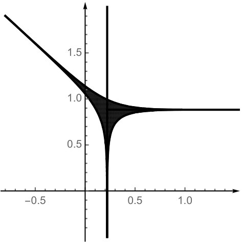 Figure 1
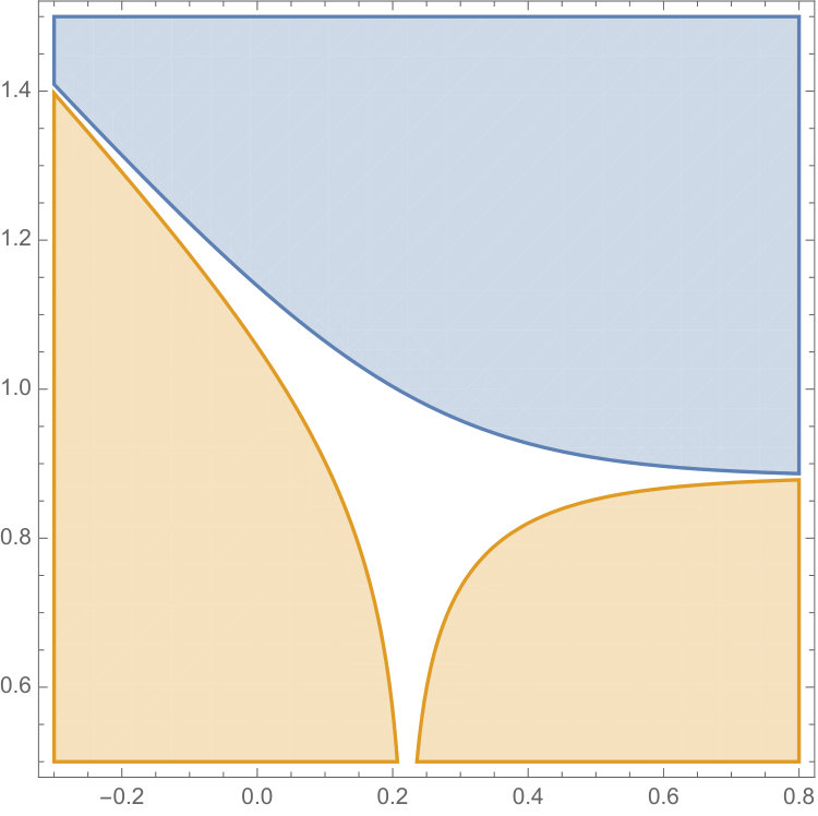 Figure 2
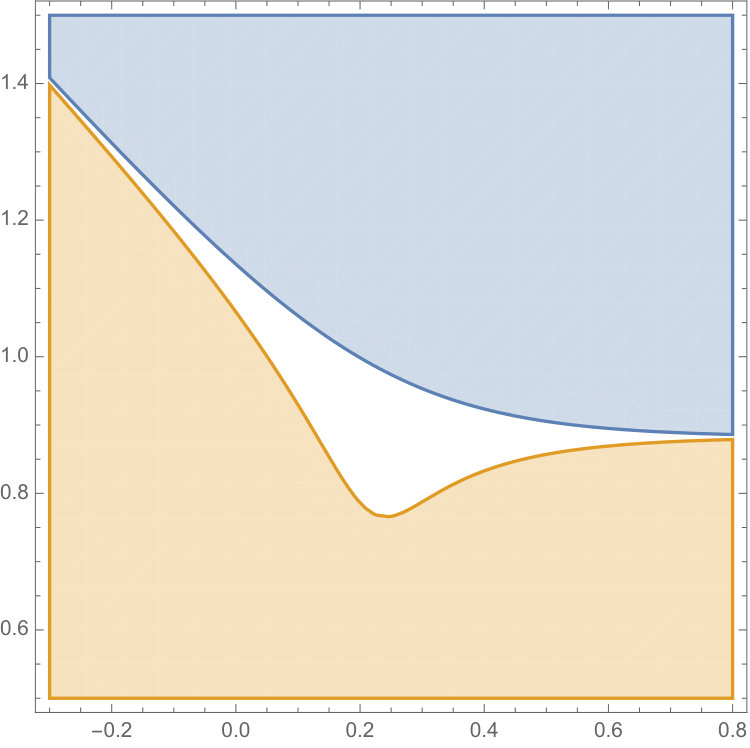 Figure 3
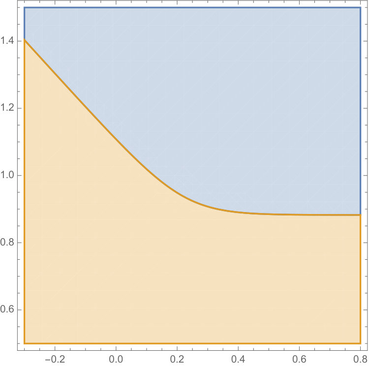 Figure 4
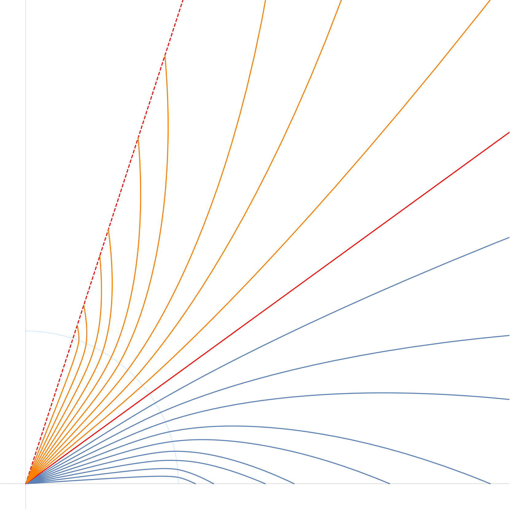 Figure 5
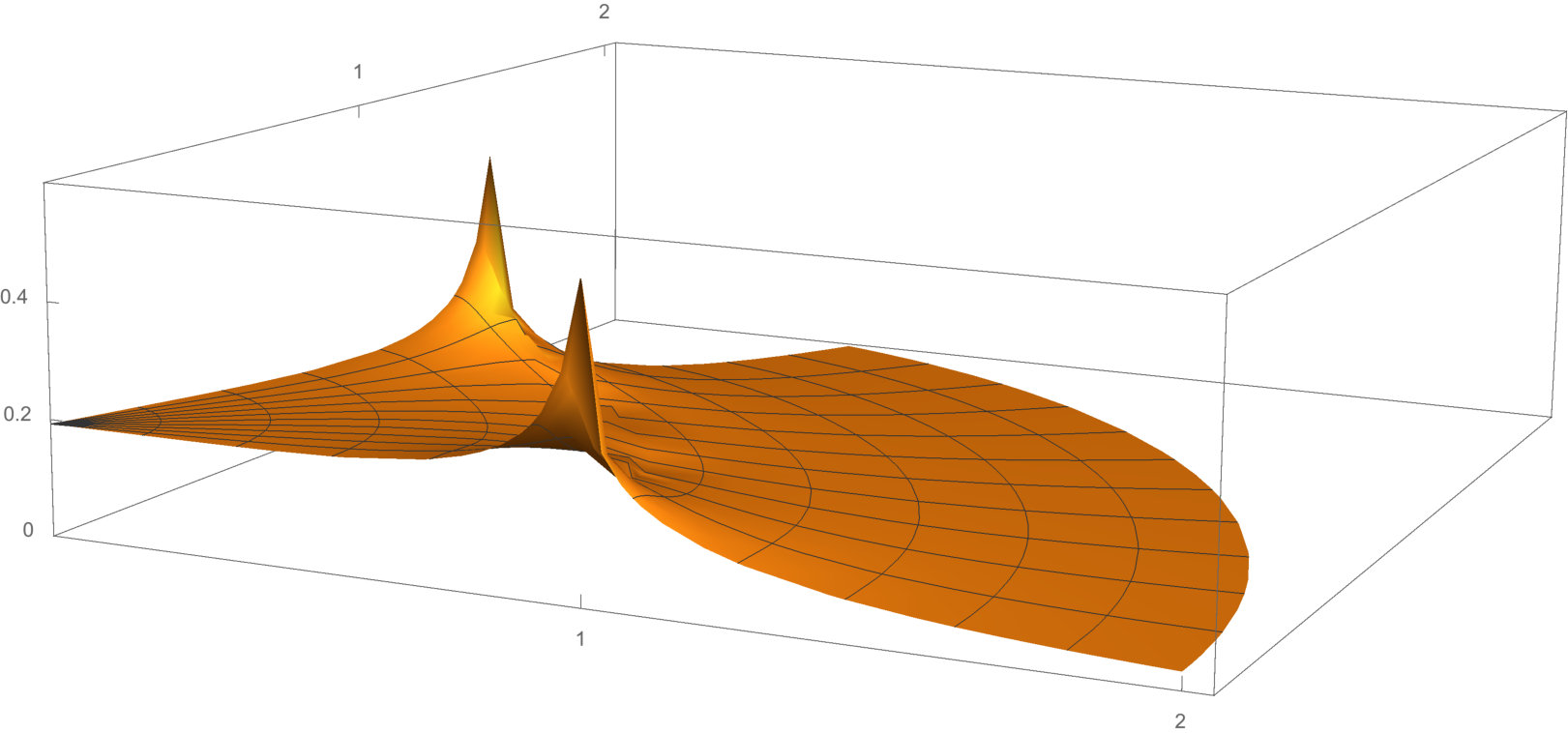 Figure 6
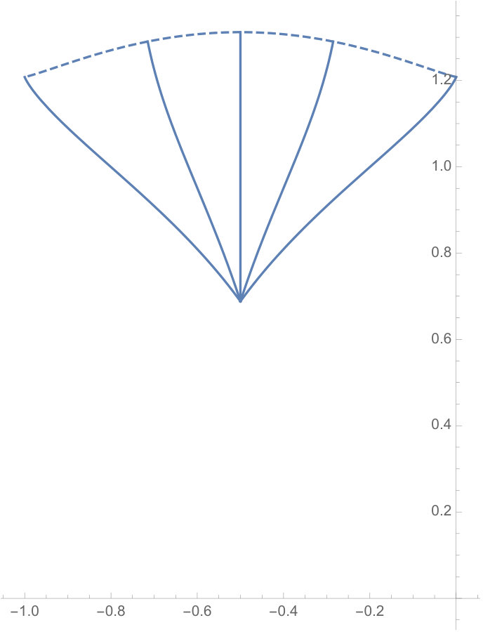 Figure 7
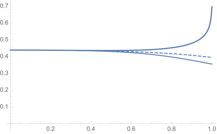 Figure 8
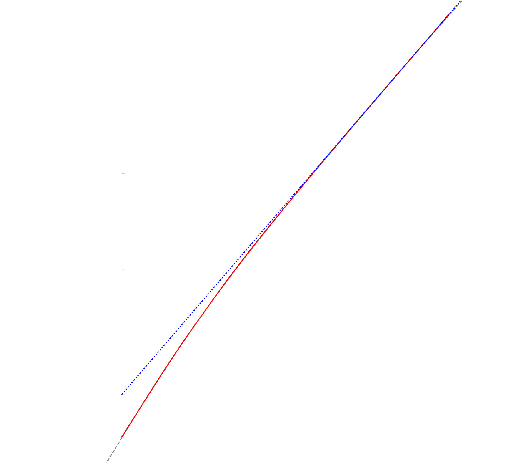 Figure 9
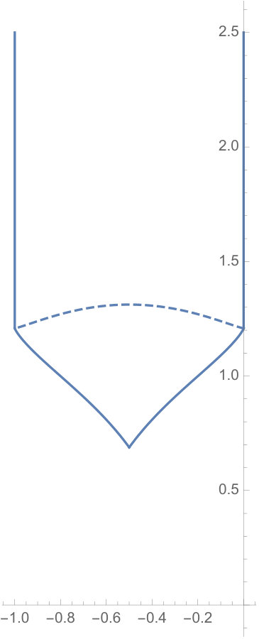 Figure 10
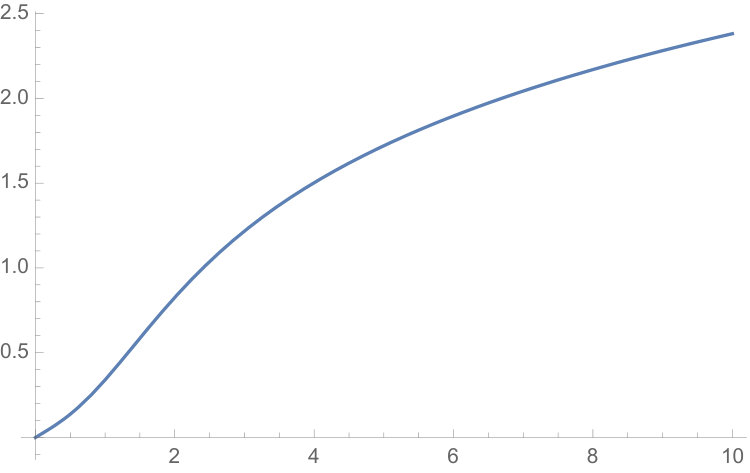 Figure 11
| model | ||
|---|---|---|
| Region | Convergence Criterion |
|---|---|
| Landau Ginzburg | and |
| Hybrid: fibration | and |
| Hybrid: orbifold | and |
| LCS | and |
| 3 | 0.1315 | 0.2043 | 0.9605 | 0.4262 | 1.3866 |
|---|---|---|---|---|---|
| 4 | 0.1127 | 0.2099 | 0.9865 | 0.4261 | 1.4125 |
| 5 | 0.0998 | 0.2213 | 0.9780 | 0.4260 | 1.4040 |
| 6 | 0.0955 | 0.2294 | 0.9567 | 0.4259 | 1.3827 |
| 7 | 0.0818 | 0.2475 | 0.9611 | 0.4259 | 1.3869 |
| 8 | 0.0877 | 0.2592 | 0.9275 | 0.4258 | 1.3533 |
| 9 | 0.0808 | 0.2825 | 0.9253 | 0.4257 | 1.3510 |
| 10 | 0.0929 | 0.3093 | 0.8969 | 0.4257 | 1.3226 |
| 11 | 0.0998 | 0.3497 | 0.8845 | 0.4257 | 1.3102 |
| 12 | 0.1234 | 0.1662 | 0.8657 | 0.4256 | 1.2914 |
| 1 | -0.081 | 0.414 | 0.957 | 0.405 | 1.362 |
|---|---|---|---|---|---|
| 2 | -0.058 | 0.347 | 0.934 | 0.404 | 1.338 |
| 3 | -0.057 | 0.329 | 0.929 | 0.402 | 1.331 |
| 4 | -0.052 | 0.319 | 0.911 | 0.400 | 1.311 |
| 5 | -0.056 | 0.327 | 0.906 | 0.399 | 1.305 |
| 6 | -0.067 | 0.347 | 0.914 | 0.398 | 1.312 |
| 7 | -0.074 | 0.368 | 0.914 | 0.397 | 1.311 |
| 8 | -0.068 | 0.389 | 0.896 | 0.396 | 1.292 |
| 9 | -0.060 | 0.423 | 0.882 | 0.396 | 1.278 |
| 10 | -0.060 | 0.459 | 0.881 | 0.395 | 1.276 |
| 11 | -0.060 | 0.502 | 0.879 | 0.395 | 1.274 |
| 12 | -0.042 | 0.283 | 0.866 | 0.395 | 1.260 |
| 1 | -0.426 | 0.747 | 0.933 | 0.225 | 1.158 |
|---|---|---|---|---|---|
| 2 | -0.409 | 0.673 | 0.920 | 0.224 | 1.144 |
| 3 | -0.399 | 0.629 | 0.908 | 0.223 | 1.130 |
| 4 | -0.393 | 0.619 | 0.893 | 0.221 | 1.115 |
| 5 | -0.398 | 0.640 | 0.892 | 0.221 | 1.113 |
| 6 | -0.409 | 0.668 | 0.900 | 0.220 | 1.120 |
| 7 | -0.417 | 0.700 | 0.904 | 0.219 | 1.123 |
| 8 | -0.414 | 0.737 | 0.893 | 0.218 | 1.112 |
| 9 | -0.409 | 0.782 | 0.883 | 0.218 | 1.101 |
| 10 | -0.410 | 0.827 | 0.882 | 0.218 | 1.100 |
| 11 | -0.408 | 0.885 | 0.878 | 0.218 | 1.096 |
| 12 | -0.388 | 0.613 | 0.865 | 0.217 | 1.082 |
| 1 | -0.655 | 1.482 | 0.949 | 0.213 | 1.162 |
|---|---|---|---|---|---|
| 2 | -0.616 | 1.289 | 0.919 | 0.212 | 1.131 |
| 3 | -0.593 | 1.179 | 0.899 | 0.210 | 1.109 |
| 4 | -0.583 | 1.151 | 0.885 | 0.210 | 1.094 |
| 5 | -0.587 | 1.182 | 0.885 | 0.209 | 1.094 |
| 6 | -0.597 | 1.219 | 0.891 | 0.208 | 1.099 |
| 7 | -0.602 | 1.263 | 0.892 | 0.208 | 1.100 |
| 8 | -0.598 | 1.322 | 0.884 | 0.207 | 1.091 |
| 9 | -0.593 | 1.392 | 0.876 | 0.207 | 1.083 |
| 10 | -0.594 | 1.449 | 0.875 | 0.207 | 1.082 |
| 11 | -0.592 | 1.522 | 0.873 | 0.207 | 1.080 |
| 12 | -0.578 | 1.195 | 0.865 | 0.206 | 1.071 |
| direction | |
|---|---|
| 0.4656 | |
| 0.0082 | |
| 0.0670 | |
| 0.0585 | |
| 0.0089 |
Peer Reviews
No public reviews on file for this paper yet. If you reviewed it on a platform where reviews are public (OpenReview, ICLR, NeurIPS, ICML), you can paste yours below so the community can read it here.
Videos
No videos yet. Explain this paper in a talk, walkthrough, or lecture? Add one.
MPP-2018-34
The Refined Swampland Distance Conjecture
in Calabi-Yau Moduli Spaces
Ralph Blumenhagen1, Daniel Klaewer1, Lorenz Schlechter2,1, Florian Wolf1
*1 Max-Planck-Institut für Physik (Werner-Heisenberg-Institut),
Föhringer Ring 6, 80805 München, Germany *
*2 Technische Universität München, Fakultät für Physik,
85748 Garching, Germany*
Abstract
The Swampland Distance Conjecture claims that effective theories derived from a consistent theory of quantum gravity only have a finite range of validity. This will imply drastic consequences for string theory model building. The refined version of this conjecture says that this range is of the order of the naturally built in scale, namely the Planck scale. It is investigated whether the Refined Swampland Distance Conjecture is consistent with proper field distances arising in the well understood moduli spaces of Calabi-Yau compactification. Investigating in particular the non-geometric phases of Kähler moduli spaces of dimension , we always find proper field distances that are smaller than the Planck-length.
Contents
1 Introduction
For relating a theory of quantum gravity, like string theory, to the real world it is of utmost importance to understand which properties of the low-energy effective action can be realized in the string theory landscape and which are outside its reach. The set of theories that cannot be consistently UV completed by a quantum gravity theory has been termed the swampland [1]. If one could make a clear statement that a certain property of the low-energy effective action cannot be realized in the landscape, this would open up the possibility of in principle falsifying string theory.
During the last years progress in this direction has been made in particular in the realm of string cosmology, where the question arose whether string theory admits controllable models of large field inflation. In such scenarios the inflaton transverses trans-Planckian field ranges and, due to the Lyth bound, gives a tensor-to-scalar ratio , i.e. values that can be measured with current and future experiments. Well motivated candidates for such models are based on axions, whose shift symmetry can protect the scalar potential against quantum gravity corrections.
However, it was argued that the Weak Gravity Conjecture (WGC) [2] provides strong constraints on models where the axion potential is generated by non-perturbative effects [3, 4, 5, 6]. In effect, the WGC implies that for models with one [7] or more axions [8, 9], increasing the field range to the trans-Planckian regime means that one moves outside the regime of a controlled low-energy effective action (see also the early work [10]).
A second approach towards realizing axion inflation is to impose a controlled spontaneous breaking of the axionic shift symmetry [11] by adding branes or fluxes. This ansatz is called axion monodromy inflation and was introduced in the stringy context in [12]. One at first sight promising mechanism to generate a polynomial potential for axion monodromy inflation is to turn on background fluxes generating a tree-level F-term scalar potential [13, 14, 15]. However, concrete attempts to realize such a scenario in a consistent scheme of string theory moduli stabilization [16, 17] showed that one encounters major obstacles. In fact, the prior assumptions about the range of validity of the low-energy effective action were violated. For instance, often one could not keep the moduli masses smaller than the Kaluza-Klein masses. A more general observation [18, 19] was that taking the backreaction of the rolling axion onto the other moduli into account, the backreacted proper field distance showed a logarithmic behavior . Here can be considered as the scale in field distance where the backreaction becomes substantial.
It was realized in [19, 20] that this logarithmic scaling of the proper field distance is very generic and that it precisely reflects one of the conjectured behaviors by Ooguri/Vafa [21] to distinguish effective field theory models that can be realized in string theory (the landscape) from those that cannot be coupled in a UV complete way to gravity (the swampland) [1].
This now called ‘Swampland Distance Conjecture (SDC)’ [22] was abstracted from the very simple example of string theory compactified on a circle, where it is the Kaluza-Klein tower that shows this behavior in terms of the proper field distance. It says that if one moves over very large distances in the moduli space of an effective quantum gravity theory, there appears an infinite tower of states whose mass scales as . This means that for the effective theory breaks down. A new field theoretic perspective on the relation between the logarithmic scaling and the infinitely many exponentially light states was recently given in [22, 23].
This paper is concerned with the question, at which scale this happens, i.e. what the size of the region where the effective theory can be trusted is. In fact, the concrete models of axion backreaction discussed in [19] always had , that is the cut-off in the field distance was close to the Planck-scale. This motivated to formulate the Refined Swampland Distance Conjecture (RSDC) [20], that extends the original one of Ooguri/Vafa by the statement that . Clearly, if this conjecture holds also for axions with a potential, it will provide a generic quantum gravity obstacle to realize axion-monodromy inflation in a controlled way using a low energy effective action. Recent discussions of the Swampland Distance Conjecture in the context of axion monodromy inflation are [24, 25, 26, 27] (see also [28] for a geometric reason for finite distances in moduli spaces).
It is the purpose of this paper to go a step back to the original work of Ooguri/Vafa and analyze the RSDC not only for moduli spaces of toroidal compactifications but for genuine Calabi-Yau (CY) compactifications of type II superstring theory. This means that the axions do not receive a potential and remain as periodic flat directions. More concretely, we will challenge the RSDC by computing proper field distances along geodesics (and sometimes non-geodesic trajectories) in the Kähler moduli spaces of Calabi-Yau manifolds. For that purpose we will use the available two methods. First one can compute the periods of the mirror dual CY manifold and second one can extract the Kähler potential from the 2-sphere partition function of the gauge linear sigma model (GLSM).
It is well known that these Kähler moduli spaces do not only contain (geometric) regions/phases, where points at infinite distance exist, but also non-geometric phases of stringy nature, like the Landau-Ginzburg (LG) phase. These often do only have a finite radius and therefore do not admit points at infinite distance. To reach the latter one first has to cross the non-geometric phase and move to another geometric phase where such a point do exist. If the distances one can travel along geodesics in such non-geometric phases were already larger than , it would directly falsify the RSDC. Therefore, our main objective is to compute geodesic distances in the moduli space of Calabi-Yau compactifications and compare them with the expectation from the RSDC. We emphasize that very similar in spirit, in [29] axion decay constants have been evaluated in the geometric phases for CY threefolds with the result that they are bounded from above by an order one parameter times the Planck-scale.
In section 2, in more detail we explain the RSDC and our approach to check it in Calabi-Yau moduli spaces. For self-consistency, section 3 contains a summary of the known techniques we employed to gain the necessary information on the moduli spaces. The reader familiar with these techniques can safely skip this section. The sections 4 and 5 are the main sections of this paper. For a couple of one and two moduli examples we analyze (geodesic) proper field distances between points in their moduli spaces and compare them with the expectation from the RSDC. In section 6, based on a recent advance [30, 31], we also investigate the full 101 dimensional Kähler moduli space of the mirror quintic. The result of this endeavor can be summarized by saying that in all instances our results are consistent with the RSDC, thus providing non-trivial evidence for it. We finally will make the compelling observation that our data seem to suggest that the finite proper field distance one can traverse in a single non-geometric phase scales inversely with the number of phases.
2 Prerequisites and objectives
Before we dwell into the more formal analysis, let us explain the objective of this paper. This is an analysis of the Refined Swampland Distance Conjecture in the moduli space of Calabi-Yau compactifications.
2.1 Basics on Calabi-Yau moduli spaces
Let us first introduce some very basics of type II compactifications on CY manifolds. Consider the compactification of type IIA superstring theory on a Calabi-Yau manifold with Hodge numbers . The four-dimensional effective theory has space-time supersymmetry. The dimension of complex structure moduli space gives rise to hypermultiplets and the dimension of the Kähler moduli space to vectormultiplets. Such a compactification is dual to type IIB compactified on the mirror CY manifold with Hodge numbers and , which gives the same massless spectrum.
Since hyper- and vectormultiplets decouple in supergravity, the vectormultiplet moduli space of the type IIB model on the mirror CY does not receive world-sheet instanton corrections and can be reliably computed at string tree-level (in ). This complex structure moduli space is mapped via mirror symmetry to the Kähler moduli space of the type IIA model. The latter indeed receives corrections which can be read-off once one knows the precise mirror map between the moduli.
In this paper we will be concerned with field distances in these vectormultiplet moduli spaces. In section 3, we will review methods to compute their Kähler potential and consequently their metric. The classic method of Candelas et al. [32] applies to the complex structure moduli space of the mirror Calabi-Yau manifold where techniques were developed to compute the periods of the holomorphic three-form and from them all the information on the (classical) complex structure moduli space. More recently, methods were developed [33, 34, 35] that work directly for the Kähler moduli space of the original CY and allow to compute the 2-sphere partition function utilizing the description in terms of gauged linear sigma models (GLSMs). From the partition function one can deduce the Kähler potential.
Of course, the two descriptions have to agree so that we are free to use either the language of the complex structure or the Kähler moduli space. Throughout this paper, we will use the Kähler moduli space, i.e. we will speak of large and small radius regime. When we say conifold locus (that is actually defined in the complex structure moduli space), we mean the mirror dual of it. As we will see in the next section, the advantage is that Kähler moduli more directly set the mass scale of the Kaluza-Klein modes.
2.2 The Refined Swampland Distance Conjecture
In this section, we briefly explain the Swampland Distance Conjecture and recall one of its motivations. In the original paper by Ooguri/Vafa [21], what later has been called the ‘Swampland Distance Conjecture’, was just one of the proposed criteria to discriminate effective field theories arising in the string landscape from those that do not admit a UV-completion, i.e. lie in the swampland. Certainly, this criterium was the most quantitative one and, as the name suggests, is about distances in field space. Let us explain its origin for the Kähler moduli space of the type IIA model on .
In the large volume regime the Kähler potential for the Kähler moduli of is given in terms of the triple intersection numbers as
[TABLE]
where the , with , denote the complexified Kähler moduli
[TABLE]
where the two-cycles are a basis of . Following a generic trajectory inside the Kähler cone , , for very large the effective Kähler potential behaves as . Hence, the Kähler metric along the trajectory becomes
[TABLE]
There might exist special trajectories for which the numerator is smaller than three but it will never be larger. The proper field distance along a trajectory is defined as
[TABLE]
which in this case becomes
[TABLE]
with . This logarithmic scaling has a dramatic consequence for the validity of the effective field theory in which the Kaluza-Klein (KK) modes are assumed to be integrated out. The generic KK mass-scale can be estimated as
[TABLE]
which implies that for trans-Planckian field excursions an infinite tower of KK-states becomes light, thus spoiling the validity of the effective field theory.
In [21] Ooguri and Vafa formulated this in a more concise manner. They provided a couple of conjectured criteria that an effective theory in the landscape necessarily should satisfy. The most quantitative criterion was termed the Swampland Conjecture in [20] and later was renamed as Swampland Distance Conjecture [22]. It says:
Swampland Distance Conjecture:
For any point in the continuous scalar moduli space of a consistent quantum gravity theory (the landscape), there exist other points at arbitrarily large distance. As the geodesic distance diverges, an infinite tower of states exponentially light in the distance appears, meaning that the mass scale of the tower varies as
[TABLE]
Thus, the number of states in the tower which are below any finite mass scale diverges as . The geodesic distance is measured with the metric on the moduli space.
In the initial version of the conjecture, is still an undetermined parameter that specifies when the exponential drop-off becomes significant. As we have seen in (2.5), for trajectories (not necessarily geodesic) in the large volume regime of CY compactifications one has .
Infinitely many states becoming exponentially light in field space indicates that the effective quantum gravity theory at the point only has a finite range of validity in the scalar moduli space. To determine the exact value of the displacement where the effective theory breaks down, all relevant mass scales have to be taken into account. Therefore, the exact upper bound on the displacement is highly model-dependent, but it is sure that in the presence of the exponential drop-off, any physics that we might derive for larger values cannot be trusted.
However, it is not a priori clear at which finite value of the distance along a geodesic this exponential drop-off first sets in. Indeed, the scale was derived already in the large radius regime without any reference to the point where the geodesic started. In [19, 26], by analyzing a couple of string theory models, evidence was provided that is equal to the natural mass scale in quantum gravity, namely 111There, the displaced field was actually an axion, hence the consequences of the SDC were only visible through backreaction effects induced by moduli stabilization.. For the simple examples chosen, all scales turned out to be related, i.e. . Let us point out that these papers focused on stabilized moduli in contrast to the original work of [21]. In the case of unstabilized moduli, general arguments were given in [20] in favor of a Refined Swampland Distance Conjecture which states that not only but also (in Planck units). In other words, for any starting point of a geodesic, one cannot follow it for a longer distance than before the validity of the effective theory breaks down.
The objective of this paper is to test this highly non-trivial conjecture in the Kähler moduli space of type IIA string compactications on CY manifolds. For that purpose we head out to compute the critical values and for a plenitude of different trajectories/geodesics in various CY manifolds. Let us explain this idea in more detail.
2.3 Objective: Testing the RSDC in CY moduli spaces
As we have recalled, the intuition for the Swampland Distance Conjecture derives from the form of the Kähler potential in the large radius regime222Other examples were presented already in [21], for example the Planck-normalized mass of the oscillator modes of the F- and D-strings as a function of the string coupling.. It is known that the Kähler moduli space of a Calabi-Yau manifold also contains non-geometric regions where corrections become important. For instance, for the quintic the form of the Kähler moduli space has the structure shown in figure 1.
As indicated, there are three distinguished points: the large volume point, the conifold and the Landau-Ginzburg (LG) point. The LG or Gepner point is the one of minimal radius. To cover the whole moduli space, one needs at least two charts, whose radii of convergence are shown by the dashed arc in figure 1.
The concrete description of this moduli space will be recalled in section 4.1. At this stage, we just want to mention that one can ask the question whether the RSDC still holds for points in the small volume regime. We will see that the conifold and LG points are at finite distance in the moduli space so that the only region featuring infinite distances is the large volume regime. Following a geodesic from the LG point to the large volume regime, one expects that the proper field distance depends on like shown in figure 2.
As long as one stays in the small volume regime the proper field distance scales polynomially with and at some point the logarithmic scaling becomes dominant. As a consequence, we define the critical field distance as the sum
[TABLE]
which includes the distance . This makes sense as we would like to know how much distance can one travel along a geodesic before the effective field theory breaks down. For the quintic example, displacing the Kähler modulus from the LG point towards the large volume phase, would be at least the proper distance to the edge of the convergence region of the LG phase, which is approximately the same as the distance between the LG and conifold point.
Clearly, if determined in this way was already larger than the Planck-scale, the RSDC would be falsified. Said the other way around, if the RSDC is correct, the proper field distance that can be traveled in the small volume regime must be smaller than . Therefore, the (proper) radius of convergence for any chart that does not contain a region of infinite distance should be sub-Planckian.
Now, let us confirm that the identification of with the radius of convergence is really a good approximation. In the case of a single modulus, the general asymptotic form of the prepotential is [32]
[TABLE]
where the constant is the one-loop contribution and the dots denote non-perturbative corrections. From this we find that the asymptotic form of the proper distance is
[TABLE]
The point where the perturbative contribution is of the same order as the asymptotic logarithm is found to be at
[TABLE]
where is the Lambert -function. For the quintic with Euler characteristic , this is approximately at , a value well below the minimal value of in the large radius phase . Indeed, at the phase boundary, the logarithm is approximately twice the size of the term, which can be considered a small correction for all larger than this. This is the case for all models that we analyzed and of course consistent with the fact that the expansion is a perturbative expansion which breaks down in the non-geometric regions of the moduli space.
As a result, the logarithm is a good approximation for the behavior of the proper distance over the whole large volume phase and only breaks down at the boundary to non-geometric regions. Thus, the only relevant contribution to comes from inside the non-geometric phases and the behavior predicted by the SDC sets in immediately after crossing the phase boundary.
It is the goal of this paper to check two very concrete predictions of the RSDC, namely that both and should be bounded by in Planck units.
3 The Kähler metric on moduli spaces
To be able to test the RSDC, for concrete examples of CY manifolds one needs the explicit form of the metric on the Kähler moduli space. In this rather technical section we describe the two employed methods to calculate this metric.
First we use the conjecture of [34] which was proven by [35]. There the Kähler potential and thereby the metric can be read-off from the partition function of a corresponding gauged linear sigma model (GLSM). Second one calculates the periods of the holomorphic three-form for the mirror CY and transforms them into an integral symplectic basis. Using two different methods allows us to also compare the numerical results.
Moreover the two methods have different advantages and disadvantages. While the GLSM construction is very efficient and mathematically easier, it is hard to extract the periods and thereby the mirror map from the partition function in the non-geometric phases. The period formalism on the other hand becomes quite involved, but from the periods one also obtains the mirror map directly.
3.1 Sphere partition function for GLSM
In the GLSM approach the Kähler potential is given in terms of the 2-sphere partition function of the gauged linear sigma model
[TABLE]
The partition function for a general GLSM was calculated in [33, 36]. In the Coulomb branch the relevant fields in the path integral are the scalar parts of the vector multiplets and the field strengths of the vector part of the vector multiplet. The index labels the vector multiplets of the theory, while the index labels the chiral fields. As the sphere is a compact space, the field strengths are quantized, with the being integers. Thus for an abelian gauge group it can be written as
[TABLE]
where the purely imaginary integration contour for the scalar fields is chosen to simplify the expressions. For an abelian gauge group is trivial. The classical contribution is
[TABLE]
and the contribution from the 1-loop determinants of the chiral fields are given by
[TABLE]
After performing the integration, the partition function only depends on the complexified Fayet-Iliopoulos (FI) parameters , and the gauge- and -charges and of the chiral fields. In the next section we describe how to identify these parameters for a given Calabi-Yau.
Data of GLSM
The GLSM is a two-dimensional supersymmetric gauge theory build out of chiral multiplets with and with . In addition there are vector multiplets . The chiral multiplets carry the charges shown in table 3.5.
[TABLE]
The fields can be considered as the homogeneous coordinates of an ambient toric variety that has identifications. The fields provide the constraints. The dimension of the resulting space is . The CY condition is related to the vanishing of the mixed gravitational - abelian gauge anomalies, which are proportional to the sum of the gauge charges
[TABLE]
In addition there exist a superpotential
[TABLE]
that is linear in the and the polynomials are such that carries vanishing charges. Moreover, one associates -charges to the chiral fields such that the superpotential has -charge . The superpotential only depends on the complex structure, therefore the A-model partition function is independent of the superpotential itself. The superpotential only restricts the value of the -charges. The -charges of the fields are determined by the condition that with the -charges of all chiral field positive. This does not uniquely fix the -charges, but the remaining freedom corresponds to a rescaling of the partition function or equivalently a Kähler transformation of the Kähler potential.
In this paper we will be concerned with for instance non-singular hypersurfaces in weighted projective spaces
[TABLE]
Since there is only a single gauge symmetry and the chiral fields carry charge , and with .
If the space is singular, the singularities have to be resolved. If this is possible by toric methods, additional gauge symmetries are added. The gauge charges of the chiral fields are in this case determined by the generators of the Mori cone, which can be calculated using the PALP package [37].
Coordinates on Kähler moduli space
The partition function (3.2) is given in terms of the FI-parameters of the GLSM used to describe the CY. We define and , where in the second definition are the complexified Kähler moduli, . While the calculations are simpler in the coordinate system, most results in the literature are stated in terms of the “algebraic” coordinates, denoted by or . These are the coefficients of the deformations of the defining polynomial in the mirror dual. To relate these coordinates to each other, one determines special points in the moduli space. These special points are the Landau-Ginzburg point at , the large complex structure point and the singular loci. In the GLSM coordinates, the singular loci are located at the solutions to the equations [38]
[TABLE]
and
[TABLE]
where denotes the VEV of the operator . Here is the scalar part of the vector multiplet. The are obtained from by setting all which are charged under a subgroup of to 0 and by only taking the uncharged chiral fields into account. The equation has to be fulfilled for all subgroups of whose charges span with positive coefficients.
In the algebraic coordinates, the manifold becomes singular at the points where the transversality condition is violated, i.e.
[TABLE]
Matching these two loci allows to fix the coordinate transformation .
The procedure is the same for all models, so we will demonstrate it in the case of the two parameter model with gauge group . The gauge charges are
[TABLE]
Inserting this into (3.9) and expressing the in terms of gives
[TABLE]
where for ease of notation . These equations have solutions if
[TABLE]
Moreover, the only subgroup of whose charges span is the first . The remaining charges are . Therefore (3.10) produces the additional relation
[TABLE]
Turning to the algebraic coordinates, the defining polynomial is
[TABLE]
Solving the system of equations (3.11) with this polynomial gives the conditions and . The equations and fix the transformation
[TABLE]
After some algebraic manipulations the remaining equations fix
[TABLE]
Note that these transformations agree with [39] up to an interchange of the indices.
Evaluating the partition function
The partition function (3.2) is of the Mellin-Barnes type
[TABLE]
where is an entire function, and are polynomials in and and are constant vectors. In the literature, numerical algorithms solving this type of integrals are described. We use the method of [40] which applies a construction of [41].
Moreover, in some phases it is possible to directly rewrite the integral as an infinite sum over residues, which will be demonstrated in the examples where it applies.
3.2 Examples
In this section we apply the methods of the sections 3.1 and 3.1 to some CY spaces. We start with the quintic, which was well studied in [32]. Second, we look at the one parameter models of [42]. Finally we study the two-parameter models of [43].
Quintic
The quintic has and is one of the simplest examples. The gauge group is . The defining polynomial is
[TABLE]
so that one chooses the superpotential
[TABLE]
and the charges . The superpotential forces the -charges to be of the form , up to the choice of a single parameter . With this choice, is limited to be taken from the open interval , such that all . The actual value of does not influence the results.
Inserting these values in the partition function (3.2) and choosing one obtains
[TABLE]
In the case , i.e. the geometric phase, one can close the contour to the left, while for , i.e. the LG phase, one closes the contour to the right. The gamma functions in the denominator cancel the poles such that only one type of gamma functions contribute in each phase. In the LG phase this is only the gamma function corresponding to the field, leading to first order poles. The partition function can be rewritten in terms of a sum over the residues at these poles. Shifting the summation index and using the identity
[TABLE]
for integer , in terms of hypergeometric functions one obtains[34]
[TABLE]
where the term is omitted.
The partition function in this LG phase does not contain any logarithms. In the large volume phase, the five chiral fields contribute, leading to fourth order poles. These result in logarithms and polygamma functions in the partition function and a quite lengthy expression. The metric following from these two partition functions is shown in figure 4. It perfectly agrees with [32].
Hypersurface in weighted projective space
There are four CYs constructed by the vanishing of a polynomial in a single weighted projected spaces with . These are , , and . The gauge charges are given by the weights of the projective space and the degree of the polynomial, , , and the -charges are given by , . The value of can be chosen in the open interval , without changing the result. To obtain the highest numerical stability one has to integrate as far away from the poles as possible, making the most stable choice. All models in this category have a similar geometry as the quintic, i.e. they consist of a geometric phase and a Landau-Ginzburg-orbifold phase with a -symmetry.
Two parameter models
In addition we look at CYs with . This class of CYs contains for example , or . In these models the charge matrix is given by the -vectors, which span the Mori cone of the given model. These are known for a great variety of CYs or can be calculate using the PALP package [37]. The gauge charges are listed in table 1.
Here, the -charges of the field is denoted and the -charge of the field corresponding to the exceptional divisor . The charges for the remaining five fields are generally determined by the superpotential condition to be
[TABLE]
for the fields with gauge charge