Reality-check for Econophysics: Likelihood-based fitting of physics-inspired market models to empirical data
Nils Bertschinger, Iurii Mozzhorin, Sitabhra Sinha

TL;DR
This paper demonstrates how likelihood-based Bayesian methods can be used to fit and compare econophysics-inspired market models to empirical data, offering a more rigorous alternative to traditional phenomenological approaches.
Contribution
It introduces a likelihood-based Bayesian fitting approach for econophysics market models using Stan, enabling systematic model comparison and improved quantitative analysis.
Findings
Likelihood-based fits outperform moment matching methods.
Econophysics models can be quantitatively compared with econometric models.
Bayesian approach facilitates principled prediction and model assessment.
Abstract
The statistical description and modeling of volatility plays a prominent role in econometrics, risk management and finance. GARCH and stochastic volatility models have been extensively studied and are routinely fitted to market data, albeit providing a phenomenological description only. In contrast, the field of econophysics starts from the premise that modern economies consist of a vast number of individual actors with heterogeneous expectations and incentives. In turn explaining observed market statistics as emerging from the collective dynamics of many actors following heterogeneous, yet simple, rather mechanistic rules. While such models generate volatility dynamics qualitatively matching several stylized facts and thus illustrate the possible role of different mechanisms, such as chartist trading, herding behavior etc., rigorous and quantitative statistical fits are still mostly…
Click any figure to enlarge with its caption.
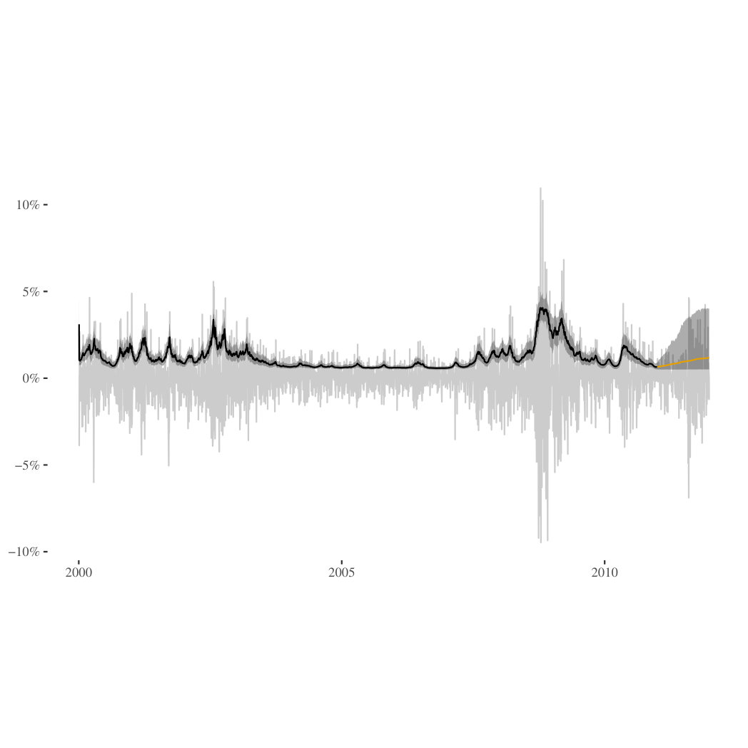 Figure 1
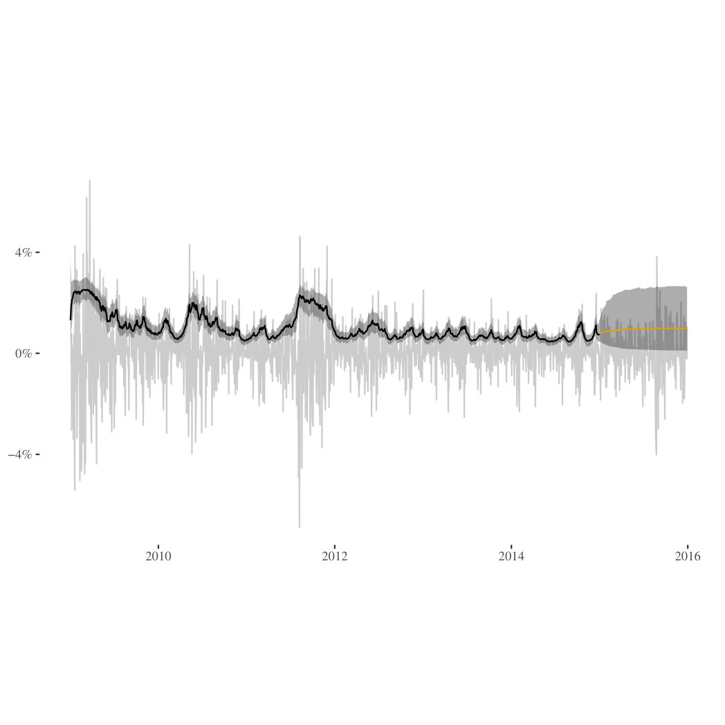 Figure 2
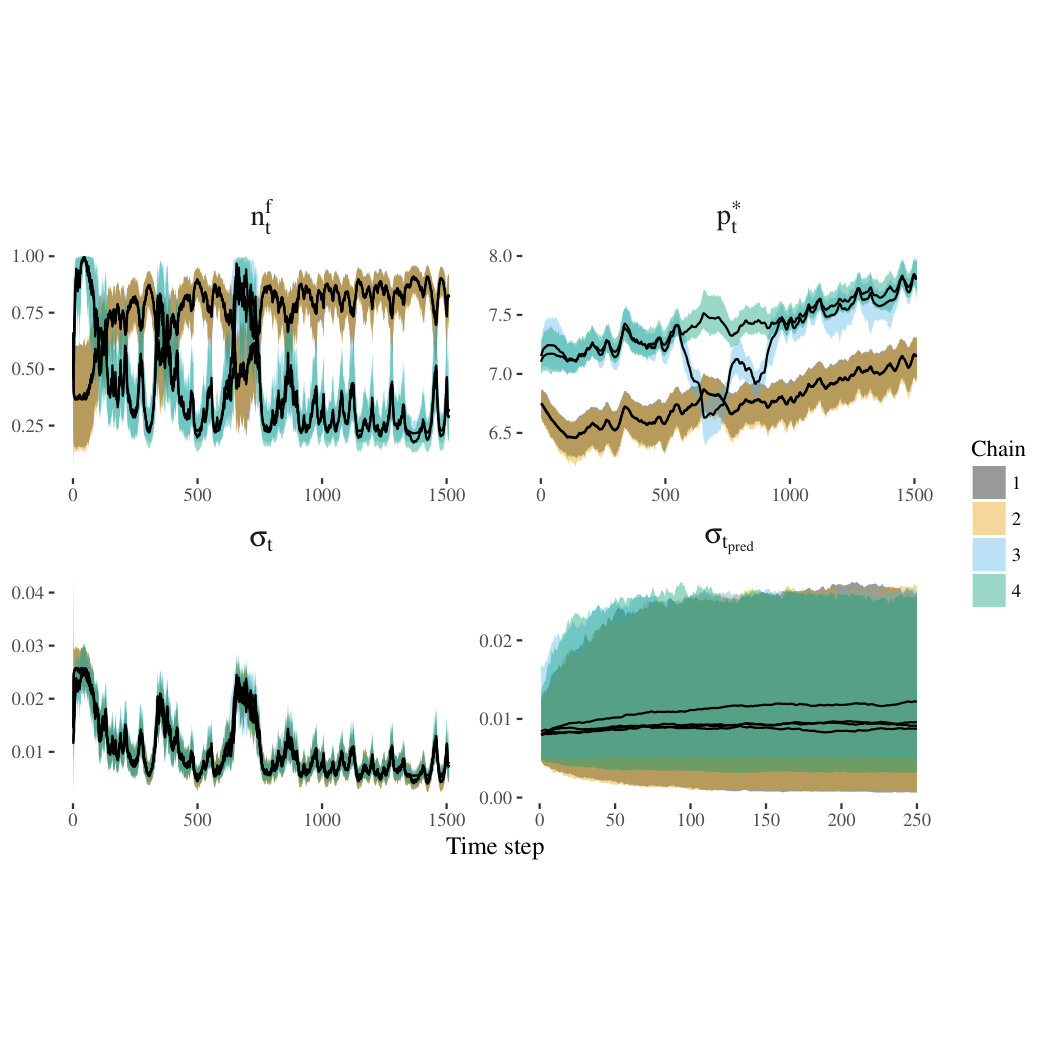 Figure 3
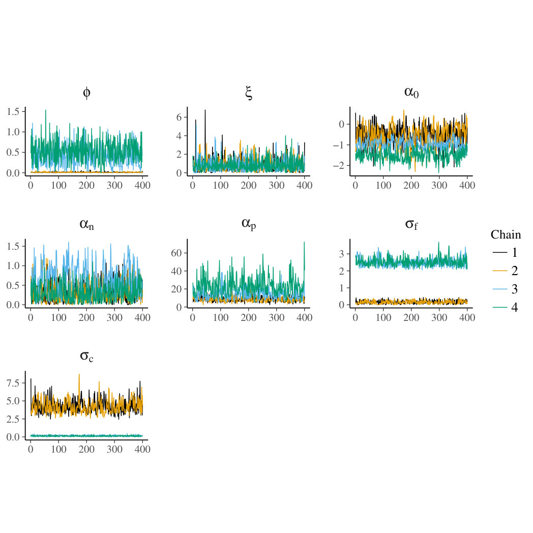 Figure 4
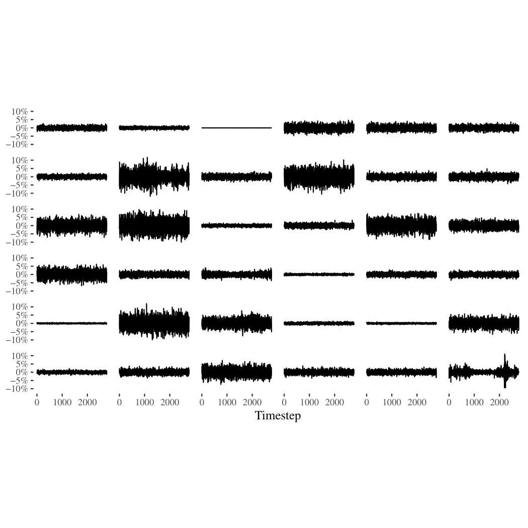 Figure 5
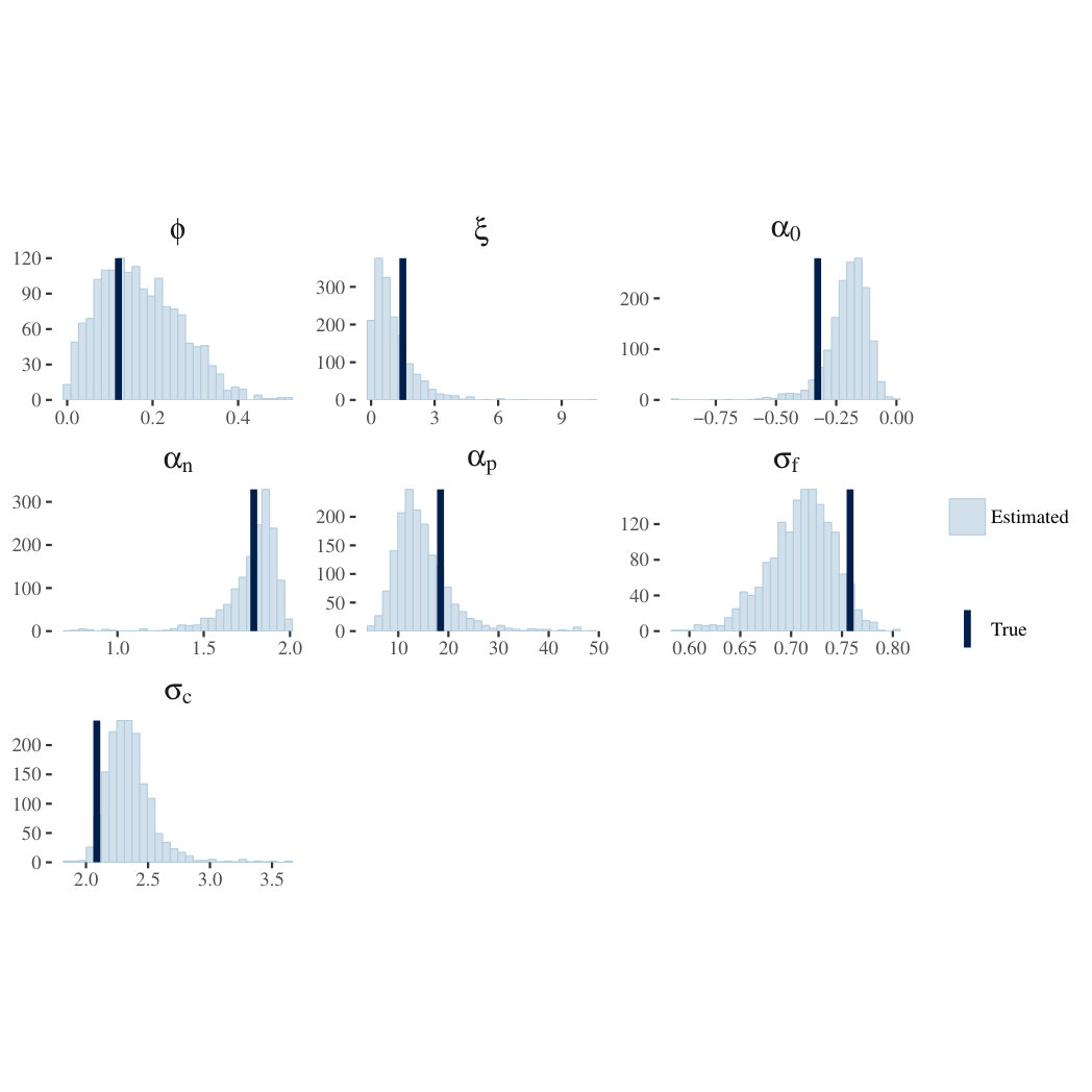 Figure 6
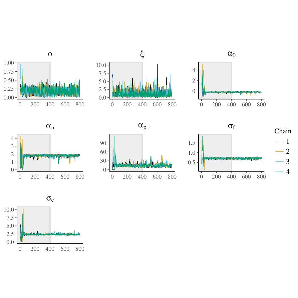 Figure 7
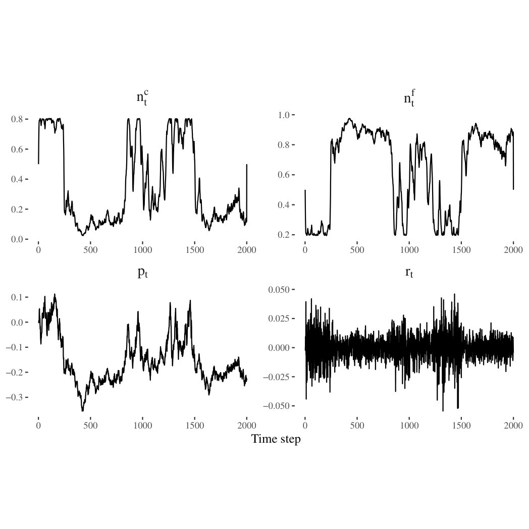 Figure 8
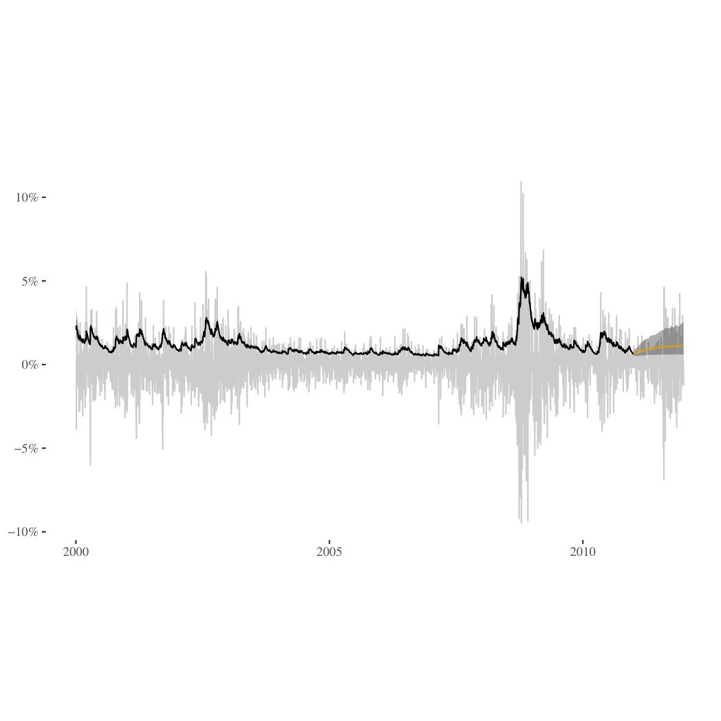 Figure 9
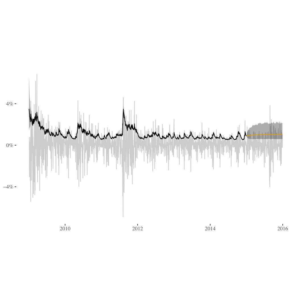 Figure 10
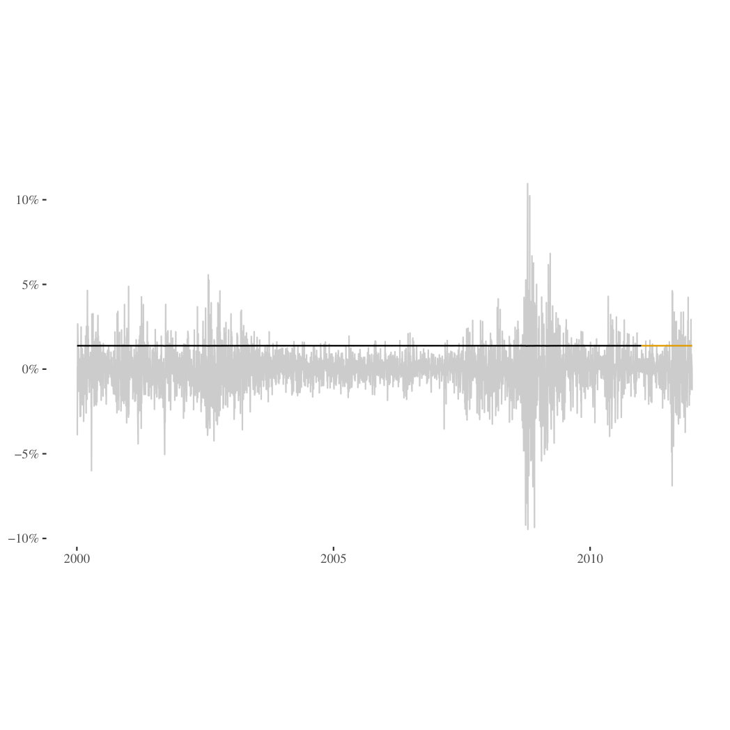 Figure 11
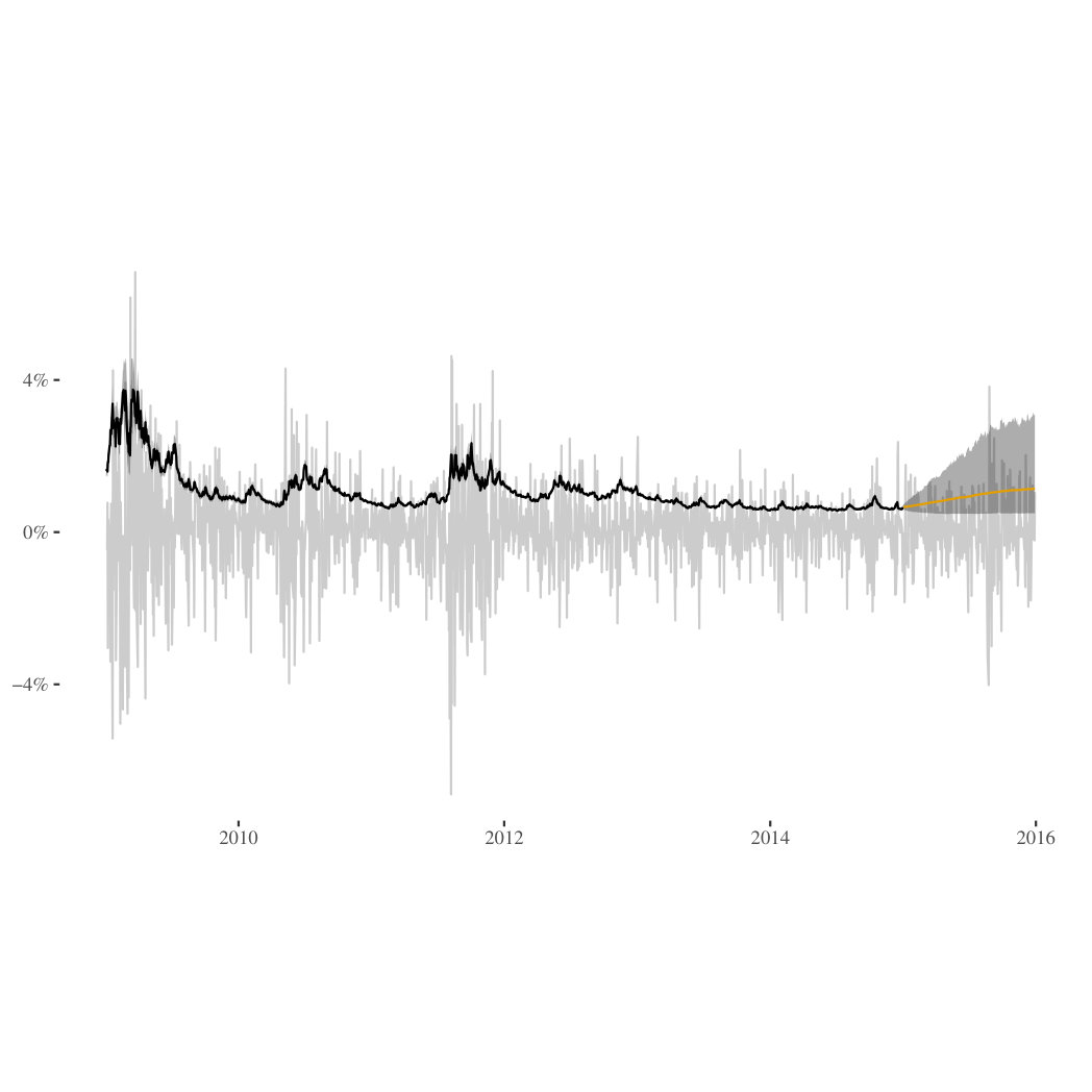 Figure 12
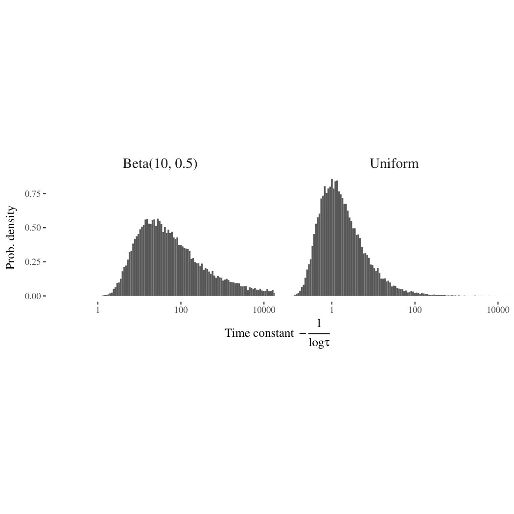 Figure 13
| Parameter | |||||||
| True | 0.12 | 1.5 | 0.758 | 2.087 | 1.79 | 18.43 | |
| Estimates | |||||||
| Mean | 0.23 | 0.97 | 0.75 | 2.14 | 1.83 | 16.9 | |
| SD | 0.23 | 0.18 | 0.056 | 0.19 | 0.14 | 0.22 | 6.0 |
| RMSE | 0.26 | 0.55 | 0.056 | 0.20 | 0.14 | 0.22 | 6.2 |
| Parameter | |||||||
| True | 0.12 | 1.5 | 0.758 | 2.087 | 1.79 | 18.43 | |
| Estimates | |||||||
| Mean | 0.23 | 0.97 | 0.75 | 2.14 | 1.83 | 16.9 | |
| SD | 0.23 | 0.18 | 0.056 | 0.19 | 0.14 | 0.22 | 6.0 |
| RMSE | 0.26 | 0.55 | 0.056 | 0.20 | 0.14 | 0.22 | 6.2 |
| Parameter | |||
|---|---|---|---|
| True | 100 | 0.999 | 0.01 |
| Estimates | |||
| Mean | 95.9 | 0.997 | 0.011 |
| SD | 11.9 | ||
| RMSE | 12.6 |
| Time window | ||
|---|---|---|
| Model | Jan. 2009 – Dec. 2014 | Jan. 2000 – Dec. 2010 |
| GARCH | ||
| VS | ||
| FW | ||
Peer Reviews
No public reviews on file for this paper yet. If you reviewed it on a platform where reviews are public (OpenReview, ICLR, NeurIPS, ICML), you can paste yours below so the community can read it here.
Videos
No videos yet. Explain this paper in a talk, walkthrough, or lecture? Add one.
Taxonomy
TopicsComplex Systems and Time Series Analysis · Financial Risk and Volatility Modeling · Time Series Analysis and Forecasting
Reality-check for Econophysics: Likelihood-based fitting of
physics-inspired market models to empirical data
Nils Bertschinger
Frankfurt Institute for Advanced Studies, Frankfurt am Main, Germany
Goethe University, Frankfurt am Main, Germany
Iurii Mozzhorin
Goethe University, Frankfurt am Main, Germany
Sitabhra Sinha
Institute of Mathematical Sciences, Chennai, India
Abstract
The statistical description and modeling of volatility plays a prominent role in econometrics, risk management and finance. GARCH and stochastic volatility models have been extensively studied and are routinely fitted to market data, albeit providing a phenomenological description only.
In contrast, the field of econophysics starts from the premise that modern economies consist of a vast number of individual actors with heterogeneous expectations and incentives. In turn explaining observed market statistics as emerging from the collective dynamics of many actors following heterogeneous, yet simple, rather mechanistic rules. While such models generate volatility dynamics qualitatively matching several stylized facts and thus illustrate the possible role of different mechanisms, such as chartist trading, herding behavior etc., rigorous and quantitative statistical fits are still mostly lacking.
Here, we show how Stan, a modern probabilistic programming language for Bayesian modeling, can be used to fit several models from econophysics. In contrast to the method of moment matching, which is currently popular, our fits are purely likelihood based with many advantages, including systematic model comparison and principled generation of model predictions conditional on the observed price history. In particular, we investigate models by Vikram & Sinha and Franke & Westerhoff, and provide a quantitative comparison with standard econometric models.
1 Introduction
Agent-based models of speculative behavior in financial markets are nowadays able to replicate many stylized facts simultaneously. Thus, providing an alternative to standard econometric models, offering behavioral explanations of observed market statistics [13, 12]. Yet, estimation of such models is still challenging and has mostly resorted to simulation based methods striving to match selected moments of the data [7, 10]. A notable exception is [14] which proposes and investigates the use of sequential Monte-Carlo methods.
Here, we follow this line of research and utilize modern software tools from machine learning and statistics to fit agent-based market models. In particular, we employ Stan [5], a probabilistic programming language for Bayesian modeling, to fit two different agent-based models, namely from Vikram & Sinha [19] and Franke & Westerhoff [8]. We believe that Bayesian estimation has many advantages as it allows to access parameter uncertainties as well as to generate model predictions. Furthermore, being based on the full model probability, including the likelihood, different models can be systematically compared, e.g. based on their predictive likelihood on held-out data.
2 Stan and Hamiltonian MCMC
2.1 Bayesian modeling
In Bayesian modeling observed data111Vectors are denoted with bold symbols throughout the text. are related to unobserved parameters/latent variables in terms of a joint probability distribution with density . This density is usually factorized as , i.e. into the parameter likelihood and prior density. Inference then rests on Bayes rule to obtain the density of the posterior distribution
[TABLE]
where the normalization is given by . The posterior summarizes the information obtained about the unobserved parameters and combines the a-priori assessment of the modeler, , with the information obtained from the data . Thus, conceptually Bayesian estimation boils down to a rather mechanical application of Bayes rule, once the full model is specified. Below, we will explain how this applies to different agent-based models and discuss, in particular, the role of prior choices in Bayesian modeling.
In practice, the normalization constant of the posterior density is often intractable, involving an integral over the parameter space. Accordingly many approximation methods have been proposed which either aim to approximate it with a tractable density or allow to draw posterior samples from its unnormalized density. Hamiltonian Monte-Carlo (HMC) sampling is an example of the latter approach. As the well known Metropolis-Hastings algorithm it is an Markov chain Monte-Carlo method, i.e. producing a sequence of possibly correlated samples. A comprehensive and readable introduction to HMC and its properties can be found in [1]. Here, a rather short overview of the method should suffice.
2.2 Markov Chain Monte-Carlo (MCMC)
Consider a target density , e.g. the posterior distribution from a Bayesian model. MCMC aims to construct a transition density which leaves the target density invariant, i.e.
[TABLE]
Such a transition density can then be utilized to draw a sequence of samples with . The well known Metropolis-Hastings algorithm uses two step in order to compute a suitable transition from :
Draw from a proposal density222Choosing a suitable proposal density is a crucial step in the Metropolis-Hastings algorithm as it controls how effectively the resulting transitions can move across the sampling space. 2. 2.
Either retain the current sample, i.e. or transition to with acceptance probability
[TABLE]
This so defined transition density not only leaves the target density invariant, but, under suitable conditions, also ensures that the chain converges to its unique invariant density starting from any initial condition [2].
2.3 Hamiltonian Monte-Carlo (HMC)
While, in theory, the Metropolis-Hastings algorithm can produce samples from the desired target density, especially in high-dimensions it can suffer from slow convergence. This arises if the proposal density is not well matched to the target density leading to either many rejected steps or small random steps diffusing slowly across the sampling space. HMC utilizes gradient information in order to generate long sweeps of proposed states which are nevertheless accepted. To this end, HMC samples from an augmented state space with density
[TABLE]
In analogy with physical systems, is considered as the momentum of a particle at position and the Hamiltonian decomposes into a sum of potential and kinetic energy respectively. The Hamiltonian dynamics, i.e.
[TABLE]
then preserves total energy/probability and thus leads to new states which can always be accepted. In practice, the above differential equation needs to be integrated numerically and care has to be taken that numerical errors do not accumulate. Fortunately, symplectic integrators can efficiently integrate Hamiltonian systems as numerical errors cancel and simulated trajectories closely approximate the theoretical dynamics. Nevertheless, as energy is only approximately conserved along numerical trajectories, in practice, HMC uses a Metropolis-Hastings step to either accept or reject the final position of a trajectory. Furthermore, before each transition a new momentum is sampled according to which is commonly taken as a Gaussian distribution independent of the current state , i.e. .
Especially in high-dimensional models, i.e. with many parameters, the use of gradient information to guide exploration is crucial to ensure efficient sampling. Note that HMC is restricted to continuous parameter spaces , but could be combined with other methods when discrete parameters are desired. Often, it is advantageous to marginalize over discrete parameters as strong correlations between them can severely hinder efficient sampling333This especially applies to Gibbs sampling. Despite its popularity Gibbs sampling is severely hindered by correlations in the posterior which can render it utterly useless in high-dimensional problems.. In theory, HMC is insensitive to strong correlations between parameters . In practice, the symplectic integrator uses a finite step size to numerically solve the Hamiltonian dynamics. In the case of posterior densities with high curvature this can prevent the sampler to reach certain parts of the state space. Furthermore, it makes HMC sensitive to the scale of parameters as the step size would need to be adjusted accordingly444In contrast, Gibbs sampling is severely effected by strong dependencies but insensitive to the scale of parameters.. Fortunately, by reparameterizing the model it is often possible to simplify the geometry of the posterior density. Furthermore, a range of diagnostics, e.g. based on the stability of the numerical trajectory, have been developed [1].
2.4 The Stan language
The probabilistic programming language Stan [5] allows the user to describe the joint probability of a model in a high-level programming language. In turn, the program is then compiled to C++ and several inference algorithms, including Hamiltonian Monte-Carlo, are build-in. The required gradients are computed via a C++ library for automatic differentiation [4], thus freeing the user from manually implementing and debugging gradient calculations.
Stan comes with an extensive documentation which includes many example models and useful tricks for efficiently implementing them [17]. A minimal Stan program consists of three blocks
a data block which declares variables corresponding to observed quantities , 2. 2.
a parameters block which declares variables corresponding to unobserved parameters 3. 3.
and a model block which contains statements computing the log density of the model, i.e. .
For instance, the following Stan program estimates the mean of Gaussian observations with a known standard deviation:
⬇ ,
1 data {
2 int<lower=0> N; // number of data points
3 vector[N] x; // observed data points
4 }
5 parameters {
6 real mu; // unobserved mean
7 }
8 model {
9 mu normal(0, 10); // computes log prior density log p(mu)
10 x normal(mu, 1); // computes log likelihood log p(x | mu)
11 // total log density is log p(mu) + log p(x | mu)
12 }
The statements in the model block relate a variable with a density and are short-hand notation for the more basic statements summing up log density contributions, e.g. target += normal_lpdf(x | mu, 1).
As shown in the example, all variables are typed and need to be declared before use. A particularly convenient feature of Stan is that variables can be given constraint types, e.g. a standard deviation parameter could be declared as real<lower=0> sigma. Internally, the variable is then automatically transformed to an unbounded space and the log density adjusted for the resulting change of measure. Due to this method many different data types including vectors, matrices but also constraint spaces such as simplices or covariance matrices are readily supported.
Stan supports several inference algorithms, namely gradient descent optimizers for maximum a-posteriori estimation, HMC sampling and stochastic gradient variational Bayes. While HMC is the least efficient of these algorithms it usually provides the closest approximation to the true posterior distribution. Furthermore, during warmup, also known as burn-in, Stan adapts several parameters of the algorithm such that the algorithm appears essentially parameter-free to the user. This is especially effective for the No U-Turn Sampler (NUTS) which automatically adjust the length of simulated trajectories. In a nutshell NUTS integrates the Hamiltonian dynamics until it starts turning back towards itself which is locally decided based on the gradient direction. Care needs to be taken to ensure that the resulting transitions leave the target density invariant. To this end, trajectories are expanded in a tree like fashion by successively doubling their length forward and backward in time. The next state is then sampled uniformly from the resulting overall trajectory.
For further details about the Stan programming language and the NUTS algorithm we refer the interested reader to the Stan manual [17] and [1] respectively. Next, we turn to agent-based models for financial markets and show how these can be expressed as statistical models.
3 Market models
Financial markets exhibit some remarkable and often surprisingly stable statistical signatures, often referred to as stylized facts [6, 13]. Most notable and researched are the properties of asset price returns exhibiting fat-tailed distributions and volatility clustering. Especially volatility, i.e. the standard deviation of returns, has received much attention in the econophysics community for its auto-correlation decaying as a power-law suggesting a long-memory process. Accordingly many models to accurately model its statistics or explain the origin of volatility correlations have been developed.
Agent-based models consider the statistical signatures of financial markets as emergent properties, i.e arising from the collective actions of many interacting traders. Thus, complementing standard economic models which, presuming rational actors, are often unable to explain the rapid changes in volatility with calm market phases interrupted by highly volatile episodes. Shiller has coined the term excess volatility hinting at these shortcomings [16]. In contrast, agent-based models allow for bounded rational actors and can often reproduce the stylized facts presuming chartist trading and/or herding behavior [15].
Here, we consider two models namely by Vikram & Sinha [19] and Franke & Westerhoff [8] in detail. In particular, we explain how these models give rise to a latent state dynamics which can be simulated and estimated with Bayesian methods.
3.1 Model by Vikram & Sinha (VS)
The market in the VS model is populated by traders. At each time step a trader either buys (), sells () or stays inactive (). The normalized net demand from all traders is then given as and the price adjusts as . An agents decision to buy/sell or staying out depends on the perceived mispricing between the current price and its running average which is considered as a proxy for the fundamental price of the asset. The probability of an agent to trade is then given by
[TABLE]
and a trading agent buys or sells at random with equal probability.
In order to obtain a statistical model of volatility, in particular with a continuous latent state as required for HMC sampling, we have adapted the model as follows:
- •
For a large number of agents the net demand converges to a Gaussian distribution with mean zero (as ) and variance
- –
Here, we have used that agents trading decisions are independent and
[TABLE]
- –
Next, considering the number of agents as unknown we introduce a scaling parameter for the variance and model the demand as .
- •
Finally, we approximate the log-return by linearizing the price impact555We have also fitted the exact model, i.e. putting a normal distribution on the transformed returns without any noticeable difference.
[TABLE]
where we have used that for .
Overall, we arrive at the following model dynamics666Simulating this approximate model shows that it produces similar price series with strong volatility clustering as the original model.
[TABLE]
Note that this is a state-space model with a continuous latent state driving the time varying volatility . Indeed, the famous GARCH(1, 1) (generalized auto-regressive conditional heteroscedastic) model [3] is of a similar form
[TABLE]
The main difference between the VS (in our formulation) and the GARCH model is that the volatility is a function of past prices in the former and past returns in the latter model. Furthermore, due to being founded in an agent-based model all parameters of the VS model are readily interpretable as the sensitivity of the agents to mispricing and the weighting of the running price average. In contrast, parameters in the GARCH model are motivated purely from statistical grounds and cannot easily be related to agent behaviors.
From a Bayesian perspective, Eq. (1) and Eq. (2) correspond to the likelihood , i.e. the conditional probability of the observed data given the model parameters. To complete the model density we need to specify a prior distribution on the parameters. The choice of a prior distribution is often considered as subjective (whereas the likelihood has an aura of objectivism). Arguably, from the perspective of modeling the observed data this distinction is of limited relevance. Instead, note that fixing the prior implicitly fixes a distribution on the data space, i.e. obtained as by marginalizing over the parameters. A model can be considered as misspecified when it assigns very low probability to the actual observed data. In contrast, a good model should be able to generate similar data with reasonable probability. This viewpoint is in line with [9] who argue that the prior can only be understood in the context of the likelihood. Indeed prior and likelihood act together in shaping the model and expressing our expectation about plausible data.
Here, we propose the use of (weakly) informative priors which take into account our knowledge about the role played by the parameters when generating data from the likelihood model. As an example, consider the parameter of Eq. (1). While it might be natural to simply assign a uniform prior777Note that uniform priors, especially on unbounded spaces, should not be considered as uninformative. On the one hand, an improper uniform prior, i.e. when it cannot be normalized, expresses a strong believe about extreme parameter values by assigning infinite probability mass to values above any finite threshold. On the other hand, they are not invariant under model reparameterization as shown in the above example., controls the time constant of the running price average, i.e.
[TABLE]
as for . Comparing this to an exponentially weighted average in continuous time, i.e.
[TABLE]
with time constant and exponential weighting kernel of unit weight, i.e. , we match with . Thus, interpreting as the time constant of the running average. Fig. (1) compares an and a prior on in terms of the induced prior on the time scale. Similarly, has been given a which assign more than of its probability mass to the interval . Together these priors inform the VS model to stay away from the boundary or where it becomes trivial, i.e. and thus . Accordingly, it cannot be expected to generate data exhibiting pronounced volatility clustering in this case and indeed, in the original reference [19], prices where averaged over time steps which is well covered by the chosen prior.
Implementing both models is straight-forward in Stan and the full code can be found in appendix A.2 and A.1 respectively.
3.2 Model by Franke & Westerhoff (FW)
Franke & Westerhoff have developed a series of models and estimated using moment matching methods [8, 7]. Here, we follow their presentation in [8] and introduce the DCA-HPM model in their terminology.
In the FW model the market is populated with two types of agents namely fundamental and chartist traders. The fraction of fundamental traders at time step is denoted by . The corresponding fraction of chartist traders is then given by . The log price, denoted by adjusts to the average demand from fundamental and chartist traders as
[TABLE]
The demand is composed of a deterministic and stochastic component. It is assumed that fundamental traders react to mispricing, i.e. the difference between and the (known) fundamental price , whereas chartist traders react to past price movement, i.e. . According to [8] the demand dynamics is modeled as
[TABLE]
Note that these demands are unobserved as only their weighted sum effects the price. While such a dynamics could be modeled by means of a stochastic latent state, in the present case it is possible to marginalize out the demand. As the sum of two normally distributed random variables is again normal, the combined demand gives rise to a stochastic model for the log return
[TABLE]
The volatility now depends on the fraction of chartist vs fundamental traders and changes over time. [8] calls this structured stochastic volatility, in analogy to structural models in economics, as the parameters of the agent-based model are grounded in behavioral terms and therefore economically meaningful.
The model is then completed by an update equation for the fraction of traders in each group. Here, we consider the DCA-HPM specification of [8] which is given by
[TABLE]
The parameter denotes the relative attractiveness of the fundamental over the chartist strategy. It includes a general predisposition and herding as well as mispricing effects. We chose this specification for two reasons:
The discrete choice approach (DCA) of Eq. (5) leads to a smoothly differentiable model density. This eases the exploration of the posterior when sampling with the HMC algorithm. 2. 2.
The herding predisposition misalignment (HPM) specification for the attractiveness Eq. (6) can be computed without access to the actual demands and . This is not true for the other specifications of [8] where the agents wealth depends on previous demands which, in turn, leads to a stochastic volatility model where (one of) the demands has to be modeled as a stochastic latent variable. For simplicity we have not considered this complication in the present paper.
Overall, the model dynamics is fully specified by Eq. (4), Eq. (5) and Eq. (6). The parameters of the model are given by . Note that and are redundant as they simply control the scale of and respectively. Thus, throughout we fix them at and as in the simulation exercise of [8].
When simulating data we further assume that the fundamental log price is known and fixed at . When estimating the model on real stock returns below, we do not know the fundamental price. In this case, following [14], we assume that the log fundamental price is time varying as a Brownian motion
[TABLE]
This not only introduces another parameter but also renders the model a stochastic volatility model, i.e. the volatility now includes a stochastic component. To see this note that depends on via and the attractiveness in turn includes the stochastic fundamental log price .
Nevertheless, implementing the model in Stan is readily possible. As before, the full code of the FW model is given in appendix A.3. Note that the time varying noise of the Brownian motion appears as an -dimensional vector (where denotes the number of observed time steps) in the parameter block. In addition, we have used a non-centered parameterization, i.e. p_star is computed from epsilon_star as a transformed parameter. Formally, we can express this as follows:
[TABLE]
instead of
[TABLE]
This is a standard example of a reparameterization which does not change the model, but helps when HMC sampling as the raw parameters all have unit scale, no matter which variance is currently sampled.
Here, we complete the model with weakly informative priors for all parameters. As few insights are available about the proper choice of the attractiveness parameters and we assign weakly informative priors, e.g. alpha_0 student_t(5, 0, 1), which restrict the scale of the parameter yet, being heavy tailed, allow substantially larger values888In contrast, a normal prior distribution would impose much more information as values larger than several tens of standard deviations are essentially ruled out.. In case of the standard deviation parameters and we impose stronger priors and resort to the observed data to set the proper scale. While not being purely Bayesian, this choice restricts the model to reasonable scales accounting for the fact that volatility could be measured in arbitrary units, e.g. percent per year. Overall, we found these priors effective in simulation studies as well as when estimating the model on stock data.
4 Results
Here, we present estimation results of the above models, both on simulated and on real price data.
4.1 Simulation studies
In order to check our model implementation, we simulated the FW model with parameters as given in table 1 of [8], i.e. and . Then, we re-estimated the model parameters999For this exercise, we have adapted the model code of app. A.3 such that the fundamental price is fixed at . This matches the data generating process as well as the calibration exercise in [8]. on the simulated price series of time steps shown in Fig. (2).
The resulting samples from the posterior distribution are shown in Fig. (3). Overall, we have run four chains starting from independent random initial conditions and drawn 400 samples from each after discarding an initial transient of another 400 samples as warmup. Compared to other studies the number of samples appears very low, but the high quality of the samples is clearly visible in the trace plots. The model appears to have converged after just about 50 samples and all chains produce almost uncorrelated samples from the same distribution. This is also confirmed by standard convergence diagnostics such as Gelman & Rubin’s , which compares the variance between and within chains, or the number of effective samples, which is based on the sample auto-correlation (not shown). If desired, more samples can easily be drawn as the shown estimation runs in a few minutes on a standard laptop.
Fig. (4) shows the resulting posterior distributions together with the true parameters that generated the data. We found that about at least 1000 observed prices are necessary to reliably recover the true parameters. Interestingly, preliminary runs on considerably longer time series of 5000 observations suggest that posterior uncertainty reduces only slightly, especially of the chartist parameters which appear harder to estimate, presumably because they become effective during episodes of high volatility only.
Similar experiments have been carried out with the VS model. Here, all parameters are precisely estimated after a few thousand observations. Especially has very small uncertainty while appears to be the least well identified parameter. A summary of our experiments for the FW and VS models can be found in table 1. Overall, we simulated 100 time series of 2000 time steps each and took the posterior means as point estimates for parameters.
The above exercises of parameter re-estimation are based on the idea that actual data had been generated from a fixed, yet unknown, set of parameters that is to be recovered. This is deeply routed in frequentist statistics where the properties of an estimator are compared by its repeated sampling properties, i.e. investigating its performance on several data sets generated from the same underlying true data generating process such as a model with fixed parameters. From a Bayesian perspective, as well as from a data modeling point of view, inference should instead be based on the observed data set alone. As explained above, a Bayesian model consists of a joint distribution on data and parameters with density . The corresponding (prior) distribution on data then captures our modeling assumption about which observations are considered plausible. Thus, from this perspective it is natural to investigate properties of this distribution and Fig. (5) shows randomly generated return series from the FW model with our chosen priors.
For comparison actual S&P 500 returns are included as the lower right sub panel. It is clearly visible that volatility clustering under the model is much less pronounced. Investigating different prior specifications, in particular trying to obtain stronger volatility clustering, reveals an intricate relationship between the scale of the volatility parameters and the typical size of the choice parameters . Indeed, looking at Eq. (6) this should not come as a surprise, as and control the expected price fluctuations which in turn set a scale for and (less directly) for . Overall, this data generating exercise not just aids in understanding the FW model and its assumption, but also suggests that would be easier interpretable if considered on a relative scale, e.g. reparameterized as where denotes the expected volatility. Leaving such explorations for future work, we now turn to fitting the models on stock returns of the S&P 500 index.
4.2 Fitting the S&P 500
Finally, we have fitted all models on price data from the S&P 500 stock market index. As a benchmark, a standard GARCH(1, 1) model has been included for comparison. The corresponding fits from Jan 2009 to Dec 2014 and Jan 2000 to Dec 2010 are shown in Fig. (6), Fig. (7) and Fig. (8). The estimated model volatility as well as prediction 250 days ahead is overlaid on the actual market returns.
Volatility estimates are shown as the posterior mean together with the credibility bands around it. The posterior of the volatility at time step is based on data points from returns observed over all data points, i.e. for . In the terminology of time series models this is known as the smoothing distribution, in contrast to the filtering distribution which is conditioned on previous observations only. In this respect, our results complement the work of Lux [14] who has used sequential Monte-Carlo to approximate the filtering distribution. In the context of time series, it is often convenient to evaluate models based on rolling look-ahead predictions. While these are readily available from the filtering distribution more work and successive re-fitting of the model would be required in our setup. In any case, predictions beyond the last observed data point are derived in the same fashion from the posterior predictive distribution with density
[TABLE]
i.e. by running the model forward based on the posterior distribution. Note that the unobserved state includes parameters as well as time varying states of the model, e.g. the instantaneous volatility or the fraction of chartist traders , rendering the predictions independent from past observations.
Comparing the volatility estimates and predictions of the different models, a few remarks are in order:
- •
The VS model appears to be severely misspecified. Quite often, especially if the chosen time window did not start out at high volatility, the best fit consists of constant volatility101010Despite the chosen informed priors striving to avoid this trivial solution.. Overall, the model appears unable to match the shape of empirical volatility clusters.
- •
The vanilla GARCH(1,1) model provides reasonable volatility estimates. Albeit the small uncertainty when predicting ahead suggests that it cannot generate the heavy tails of empirical returns111111Of course, this is well known and addressed by many extensions of the model.. It still provides a reasonable benchmark to compare the presented agent-based models against.
- •
Overall, the FW seems to fit the data best. In particular, the wider prediction intervals indicate its ability to generate heavy tailed return series. Due to the stochastic volatility process arising from the Brownian motion modeling the unobserved fundamental price, uncertainty of its volatility estimates is higher than for the other models. This feature is shared with other, more standard stochastic volatility models [11].
Having compared the models graphically, we proceed with a more principled assessment of model fit. In general, the predictive likelihood will be biased upwards when evaluated on the data used to estimate parameters and, in the case of nested models, prefers the more complex variants as these cannot fit the data worse than restricted variants. Thus, a fair assessment should address the models ability to predict new data. In a time series context it is rather natural to consider (running) look-ahead predictions. Here, for computational reasons, we instead resort to leave-one-out (LOO) predictions, i.e. predicting current returns in the context of past and future returns, excluding the current one. With the method of Pareto smoothed importance sampling (PSIS) [18] the corresponding predictive likelihoods can be estimated from posterior samples. Note that in contrast to the full posterior , the LOO likelihood is conditioned on all but the th data point. Thus, in order to estimate the LOO likelihood from posterior samples the th data points needs to be effectively removed before evaluating the prediction. In general, this is far from trivial and we refer the reader to [18] for details about how PSIS estimates LOO likelihood. Here, we simply give the results of model comparison in table 2. They confirm our previous analysis, that the FW model fits the data best followed by the GARCH model. The VS model seems worst even when estimating non-constant volatility.
How does the FW model achieve such a good fit of the time varying volatility? This is particularly interesting, as its parameters are interpretable in behavioral terms.
With simulated parameters, high volatility arises if the fraction of chartists increases as these are assumed to have more volatile demand, i.e. . Looking at the trace plots for the model parameters when estimated on S&P 500 returns from Jan. 2009 to Dec. 2014 reveals a surprise. The upper panel of Fig. (9) shows that chains starting from different initial conditions have not converged to the same distribution. This suggests a multi-modal posterior where each chain samples from a well defined, yet different, mode of the distribution. Furthermore, in at least one of the modes we find that !
The lower panel of Fig. (9) shows the corresponding time series of the models state variables, i.e. and . Interestingly, the model offers two very different explanations for the observed volatility dynamics. In the first scenario, the number of chartists is usually low and rises sharply in volatile market phases (as intended by the model). In contrast, in the second scenario the number of chartists is usually high and drops in volatile market phases. Volatility is then driven by the high demand uncertainty of fundamental traders. Interestingly, both scenarios lead to very similar estimates and predictions for the volatility . The model accomplishes this by assuming a very different trajectory for the unobserved Brownian motion of the fundamental price leading in turn to very different mispricings and demands of the fundamental traders. Thus, the seemingly innocuous assumption that the fundamental price follows a Brownian motion apparently introduces a symmetry into the model. This not only makes the unobserved latent states of the model unidentifiable, but also reveals that our understanding of agent-based models and their generated time series dynamics is far from complete. Further work is certainly needed in order characterize and ideally remove this unidentifiability121212At least if an interpretation of the latent state dynamics is desired. Identifiability is of no concern when deriving predictions..
5 Conclusion
We have demonstrated, using two different econophysics models as examples, that agent-based models can readily be fitted with current machine learning tools. In particular, we have implemented several models in Stan, a modern probabilistic programming language for Bayesian modeling. Furthermore, we showed that HMC sampling appears to be well suited to explore the posterior distributions arising in these agent-based models. HMC not only mixes rapidly, but also reveals clear multi-modality in the case of the FW model.
While HMC is restricted to continuous state spaces131313This apparent restriction can be overcome by marginalizing over discrete state, i.e. summing them out. [17] illustrates this approach on several examples including Gaussian mixture models and hidden Markov models., we have shown that different models are either already in this form (FW model) or can be approximated accordingly (VS model). In this regard, our work complements the study by Lux [14] who has specifically focused on modeling individual agents employing SMC methods to track the resulting discrete state dynamics. We believe that HMC has several advantages. In particular, it is highly efficient and able to handle models with many parameters such as stochastic time varying state variables, e.g. the fundamental price in the FW model. Furthermore, it provides additional diagnostics, e.g. based on the numerical quality of the integrated Hamiltonian dynamics, to access convergence and sample quality.
Here, we applied HMC to estimate agent-based models by conditioning them on several years of S&P 500 returns. The resulting posterior distribution allows to access latent state variables, e.g. time varying volatility, and derive model predictions without further approximations. Also the precision of all estimated parameters is readily available. Finally, comparing model fits by their LOO predictive likelihood, we found that the VS model appears severely misspecified whereas the FW model is on par with purely statistical econometric models outperforming a standard GARCH model. We are optimistic that, given the comparable ease with which all models could be implemented in Stan, more such attempts will be undertaken and plan to investigate further models together with more detailed comparisons in the future.
Acknowledgments
NB thanks Dr. h. c. Maucher for funding his position.
Appendix A Stan code
A.1 GARCH model
A.2 VS model
A.3 FW model
The reference list from the paper itself. Each links out to its DOI / PubMed record.
- 1[1] M. Betancourt. A Conceptual Introduction to Hamiltonian Monte Carlo. Ar Xiv e-prints , January 2017.
- 2[2] Christopher M. Bishop. Pattern Recognition and Machine Learning . Information Science and Statistics. Springer, 2011.
- 3[3] Tim Bollerslev. Generalized autoregressive conditional heteroskedasticity. Journal of Econometrics , 31(3):307 – 327, 1986.
- 4[4] B. Carpenter, M. D. Hoffman, M. Brubaker, D. Lee, P. Li, and M. Betancourt. The Stan Math Library: Reverse-Mode Automatic Differentiation in C++. Ar Xiv e-prints , September 2015.
- 5[5] Bob Carpenter, Andrew Gelman, Matthew Hoffman, Daniel Lee, Ben Goodrich, Michael Betancourt, Marcus Brubaker, Jiqiang Guo, Peter Li, and Allen Riddell. Stan: A probabilistic programming language. Journal of Statistical Software, Articles , 76(1):1–32, 2017.
- 6[6] R. Cont. Empirical properties of asset returns: stylized facts and statistical issues. Quantitative Finance , 1(2):223–236, 2001.
- 7[7] Reiner Franke and Frank Westerhoff. Estimation of a structural stochastic volatility model of asset pricing. Computational Economics , 38(1):53–83, Jun 2011.
- 8[8] Reiner Franke and Frank Westerhoff. Structural stochastic volatility in asset pricing dynamics: Estimation and model contest. BERG working paper series on government and growth , 78, 2011.