Efficient Enumeration of Bipartite Subgraphs in Graphs
Kunihiro Wasa, Takeaki Uno

TL;DR
This paper introduces the first efficient algorithms for enumerating all bipartite subgraphs in a graph, significantly advancing the computational methods for this fundamental graph class.
Contribution
It presents two novel algorithms for bipartite subgraph enumeration, one with $O(k)$ time per solution and another with $O(1)$ time per solution.
Findings
Algorithms enumerate all bipartite induced subgraphs efficiently
Enumeration time is $O(k)$ per solution for induced subgraphs
Enumeration time is $O(1)$ per solution for all bipartite subgraphs
Abstract
Subgraph enumeration problems ask to output all subgraphs of an input graph that belongs to the specified graph class or satisfy the given constraint. These problems have been widely studied in theoretical computer science. As far, many efficient enumeration algorithms for the fundamental substructures such as spanning trees, cycles, and paths, have been developed. This paper addresses the enumeration problem of bipartite subgraphs. Even though bipartite graphs are quite fundamental and have numerous applications in both theory and application, its enumeration algorithms have not been intensively studied, to the best of our knowledge. We propose the first non-trivial algorithms for enumerating all bipartite subgraphs in a given graph. As the main results, we develop two efficient algorithms: the one enumerates all bipartite induced subgraphs of a graph with degeneracy in time…
Click any figure to enlarge with its caption.
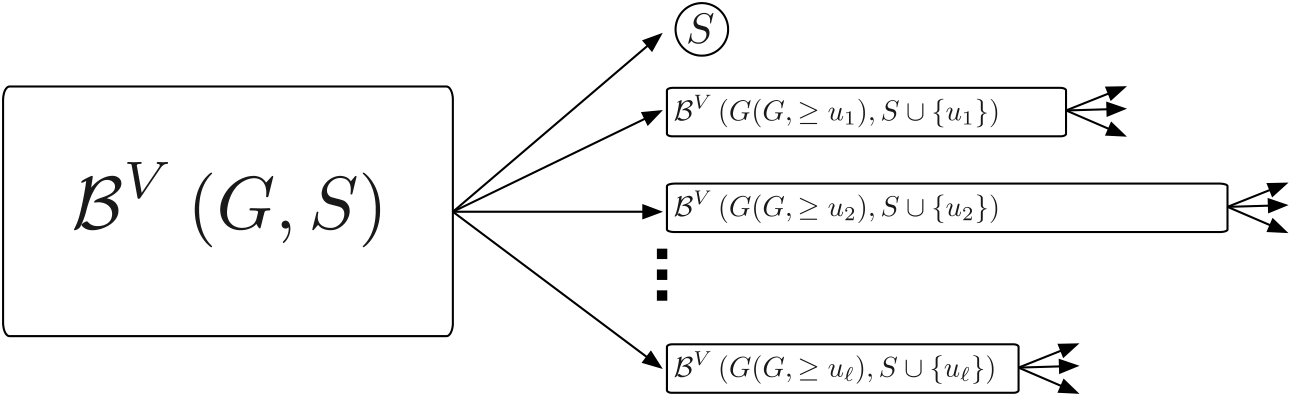 Figure 1
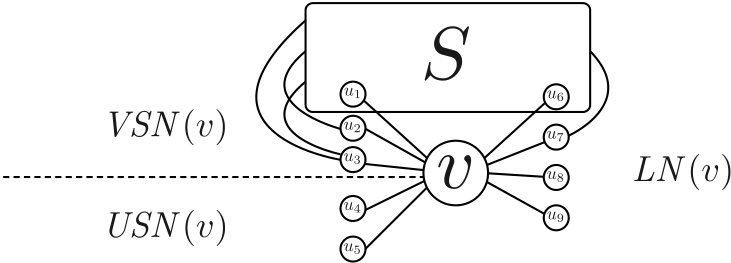 Figure 2
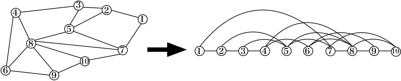 Figure 3
Peer Reviews
No public reviews on file for this paper yet. If you reviewed it on a platform where reviews are public (OpenReview, ICLR, NeurIPS, ICML), you can paste yours below so the community can read it here.
Videos
No videos yet. Explain this paper in a talk, walkthrough, or lecture? Add one.
11institutetext: National Institute of Informatics, Tokyo, Japan
{wasa, uno}@nii.ac.jp
Efficient Enumeration of Bipartite Subgraphs in Graphs
Kunihiro Wasa 11
Takeaki Uno 11
Abstract
Subgraph enumeration problems ask to output all subgraphs of an input graph that belongs to the specified graph class or satisfy the given constraint. These problems have been widely studied in theoretical computer science. As far, many efficient enumeration algorithms for the fundamental substructures such as spanning trees, cycles, and paths, have been developed. This paper addresses the enumeration problem of bipartite subgraphs. Even though bipartite graphs are quite fundamental and have numerous applications in both theory and application, its enumeration algorithms have not been intensively studied, to the best of our knowledge. We propose the first non-trivial algorithms for enumerating all bipartite subgraphs in a given graph. As the main results, we develop two efficient algorithms: the one enumerates all bipartite induced subgraphs of a graph with degeneracy in time per solution. The other enumerates all bipartite subgraphs in time per solution.
Keywords:
Graph algorithms, subgraph enumeration, bipartite graphs, constant delay, binary partition method, degeneracy
1 Introduction
A subgraph enumeration problem is, for given a graph and a constraint , to output all subgraphs of that satisfy once for each and without duplication. An example is to enumerate all the trees in the given graph, and all the subgraphs whose minimum degree is at least . The complexity and polynomiality of the subgraph enumeration have been intensively studied in theoretical computer science in the terms of both output size sensitivity and input size sensitivity. Compared to optimization approach, enumeration has an advantage on exploring and investigating all possibilities and all aspects of the data, thus is widely studied in a practical point of view, e.g. Bioinformatics [1], machine learning [18], and data mining [22, 26]. We say that an enumeration algorithm is efficient if the algorithm is output sensitive [11]. Especially, we say that runs in polynomial amortized time, if the total running time of an enumeration algorithm is time, where is the number of solutions, is the size of input, and is a polynomial function. That is, enumerates all solutions in time per solution. Such algorithms have been considered to be efficient, and one of our research goals is to develop efficient enumeration algorithms. As far, there have been studied enumeration algorithms for many fundamental graph structures such as spanning trees [17, 19], -paths [17, 7], cycles [17, 2, 8], maximal cliques [15, 6, 3], minimal dominating sets [12], and so on. See the comprehensive list in [23] of this area. Recently, Uno [21] developed a technique for a fine-grained analysis of enumeration algorithms.
Bipartite graph is a well-known fundamental graph structure. A bipartite graph is a graph containing no cycle of odd length, that is, whose vertex set can be partitioned into two disjoint independent sets. Bipartite graphs widely appears in real-world graphs such as itemset mining [26, 22], chemical information [13], Bioinformatics [27], and so on. Further, enumeration problems for matchings [10, 20, 9] and bicqliue [15, 4] in bipartite graphs are well studied. However, to the best of our knowledge, there has been proposed no non-trivial enumeration algorithm for bipartite subgraphs.
In this paper, we propose efficient enumeration algorithms for bipartite induced subgraphs and bipartite subgraphs. For enumerating both substructures, we employ a simple binary partition method, and develop a data structure for efficiently updating the candidates that are called child generators. Intuitively speaking, child generators are vertices or edges such that adding them to a current solution generates another solution. For bipartite induced subgraph, we look at the degeneracy [14] of a graph. The degeneracy of a graph is the upper bound of the minimum degree of any its subgraph, so the graph is sparse when the degeneracy is small. It is a widely considered as a sparsity measure [24, 3, 5, 25]. There are several graph classes have constant degeneracies, e.g., forests, grid graphs, planar graphs, bounded treewidth graphs, -minor free graphs with some fixed , and so on [14]. In addition, Real-world graphs such as road networks, social networks, and internet networks are said to often have small degeneracies, or do so after removing a small part of vertices. Our algorithm utilizes a good ordering on the vertices called a degeneracy ordering [16], that achieves amortized time per solution, where is the degeneracy of an input graph. This implies that when we restrict the class of input graphs, such as planar graphs, the algorithm runs in constant time per solution and is optimal in the sense of time complexity. Next, for developing an algorithm for bipartite induced subgraph, we show that we can avoid redundant edge additions and removal to obtain a solution from another solution. As a main result, we give an optimal enumeration algorithm, that is, the algorithm runs in constant time per solution. These algorithms are quite simple, but by giving non trivial analysis, we show the algorithms are efficient. These are the first non-trivial efficient enumeration algorithms for bipartite subgraphs.
2 Preliminaries
Let be an undirected graph with vertex set and edge set . An edge is denoted by . We say that and are endpoints of , and is adjacent to if . When the graph is undirected, . Two edges are said to be adjacent to each other if a vertex is an end point of both edges. The set of neighbors of is the set of vertices that are adjacent to and is denoted by . For any vertex subset of , , that is, is the set of edges whose both endpoints are in . For any edge subset of , , that is, is the collection of endpoints of edges in . The induced graph of by is and is denoted by . is a subgraph of by . We denote by . Since (resp. ) is uniquely determined by (resp. ), we identify with (resp. with ) if no confusion arises.
We say that a sequence of vertices in is a path of between and if for each , , and each vertex in appears exactly once. We denote by the length of a path the number of edges in the path. is a cycle if and the length of is at least three. The distance between and is the We say is connected if there is a path between any pair of vertices in . is bipartite if has no cycle with odd length. For a vertex subset (resp. an edge subset ) such that (resp. ) is bipartite, we say (resp. ) a bipartite vertex set (resp. a bipartite edge set). For any bipartite vertex set , if is connected, we say a connected bipartite vertex set. We also say a bipartite edge set is a connected bipartite edge set if is connected. Let and be the collection of connected bipartite vertex sets and connected bipartite edge sets, respectively. We call (resp. ) the solution space for Problem 1 (resp. for Problem 2). Since we only focus on connected ones, we simply call a connected bipartite vertex (resp. edge) set a bipartite vertex (resp. edge) set. In what follows, we assume that is connected and simple. We now define the enumeration problems of this paper as follows:
Problem 1 (Bipartite induced subgraph enumeration)
For given a graph , output all vertex sets in without duplication.
Problem 2 (Bipartite subgraph enumeration)
For given a graph , output all subgraphs in without duplication.
3 Enumeration of Bipartite Induced Subgraphs
In this paper, we propose two enumeration algorithms for Problem 1 and Problem 2, and this section describes the algorithm for Problem 1. The pseudocode of the algorithm is described in Algorithm 1. We employ binary partition method for constructing the algorithms. The algorithm outputs the minimal solution to be output, and partition the set of remaining solutions to be output into two or more disjoint subsets. Then, the algorithm recursively solve the problems for each subset, by generating recursive calls. We call this dividing step excluding recursive calls (Line 1 in Algorithm 1) an iteration.
For any pair and of iterations, is the parent of if is called from and is a child of if is the parent of .
For any bipartite vertex set , we say that is a child of if there exists a vertex such that . A vertex is a child generator of for if is a bipartite vertex set in . That is, the proposed algorithm enumerates all bipartite vertex sets by recursively adding a child generator to a current bipartite vertex set . We denote by the set of child generators of in . Suppose that be the smallest vertex in . Let and . For any vertex in , any descendant iteration of Rec() does not output a bipartite vertex set including vertices less than . Hence, no vertex will never move to the other side in any descendant bipartite vertex set. Let and . Note that , where is the disjoint union of and . We denote by the collection of bipartite vertex sets which include . Note that . From now on, we fix a graph and a bipartite vertex set of . By the following lemma, the algorithm divides according to (Fig. 1). For an edge , we define by .
Lemma 1
* for any of .*
Proof
Without loss of generality, we can assume that . Suppose that is a bipartite vertex set in . This implies that includes both and . However, does not contain . Thus, , and this contradicts the assumption. Hence, the statement holds.
Lemma 2
.
Proof
If , then is obviously in . We assume that and . This implies that includes one of child generators in . Let be the smallest child generator in such that belongs to . Hence, . Therefore, and the statement holds.
Next, we consider the correctness of ComputeChildGen. For brevity, we introduce some notations: Let be a child generator in . is the set of vertices that are adjacent to only in . Note that . if ; if . Intuitively, and are the set of vertices that are added to and removed from to compute , respectively. The following lemma shows the sufficient and necessary conditions for computing .
Lemma 3
**
Proof
We let . Suppose that . Without loss of generality, we can assume that . From the definition of , . If , then since can be added to , is adjacent to only one vertex in . Hence, . If , then since , . Moreover, if is in , then has an odd cycle. Hence, the statement holds.
Suppose that . Without loss of generality, we can assume that . Since , is connected. Suppose that has an odd cycle . Since is bipartite, must contain . This implies that has neighbors both in and . If , then has exactly one neighbor in since . Hence, . This implies that either (I) or (II) . If (I) holds, then has neighbors only in on since and . If (II) holds, then then has neighbors only in on since . Both cases contradict that in . Hence, and the statement holds.
From the above discussion, we can show the correctness of our algorithm.
Lemma 4
Algorithm 1 correctly enumerates all bipartite vertex sets in .
Proof
From Line 1 to 1, the algorithm divides the solution space according to as shown in Lemma 2. In addition, from Lemma 3, ComputeChildGen correctly computes the sets of child generators of where is a child of . Hence, the statement holds.
3.1 Update of child generators
In this section, we consider the time complexity for the maintenance of the sets of child generators. If we naïvely use Lemma 3 for ComputeChildGen, we can not achieve amortized time per solution. To overcome this, we use a degeneracy ordering on vertices. is a -degenerate graph [14] if for any induced graph of , has a vertex whose degree is at most (Fig. 2). The degeneracy of is the smallest such that is -degenerate. Every -degenerate graph has a degeneracy ordering on . The definition of a degeneracy ordering is that for any vertex in , the number of neighbors of that are larger than is at most . By recursively removing a vertex with the minimum degree, we can obtain this ordering in linear time [16]. Note that there are many degeneracy orderings for a graph. In what follows, we pick one of degeneracy orderings of and then fix it as the vertex ordering of . For any two vertices in , we write if is smaller than in the ordering. We can easily see that if is the smallest child generator, then has at most neighbors in since is -degenerate. Therefore, Lemma 3 implies that we can compute the child generators of by removing at most vertices and adding some vertices that generate some grandchildren of .
Next, we define the three types of neighbors of a vertex in , larger neighbors, visited smaller neighbors, and unvisited smaller neighbors: For any vertex , (1) is a larger neighbor of if , (2) is a visited smaller neighbor of if and , and (3) is an unvisited smaller neighbor otherwise (Fig. 3). Intuitively, is a visited smaller neighbor if one of its neighbor is already picked in some ancestor iteration of which receives . We denote by , , and the sets of larger neighbors, visited smaller neighbors, and unvisited smaller neighbors of , respectively. In addition, the algorithm divides into two disjoint parts and ; and . We omit if no confusion arises.
We now consider the data structure for the algorithm. For each vertex , the algorithm stores , , , and in doubly linked lists. is also stored in a doubly linked list and sorted by the degeneracy ordering. The algorithm needs space for storing these data structures. The algorithm also records the modification when an iteration calls a child iteration . Let (resp. ) be bipartite vertex sets received by (resp. ). Note that for each neighbor of a vertex , if moves from to , then will never moves from the list in any descendant of . Moreover, when moves to , becomes a child generator of , and thus, . Initially, for all smaller neighbors of is in . In addition, will be never added to the set in any descendant of if is not a child generator of . Hence, the algorithm totally needs space for storing the modification history. When the algorithm backtracks to from , the algorithm can completely restore the data structure in the same complexity as the transition from to . Now, we consider the time complexity for the transition from to . Suppose that when we remove a vertex from or add to , for each larger neighbor of , we give a flag which represents is not a child generator of the child of . This can be done in time per vertex because of the degeneracy. The next technical lemma shows the number of the larger neighbors which are checked for updating the set of child generators.
Lemma 5
* has at most one larger neighbor of for any vertex in .*
Proof
Suppose that two or more neighbors of are in . Let and be two of them such that is added after , and be an ancestor bipartite vertex set of for some graph such that and . Without loss of generality, we can assume that and are child generators of . We can also assume that is added after . Then, from Lemma 3, When is added to , is not in since . This contradicts, and thus, the statement holds.
Lemma 6
Let and be two vertices in such that and . can be computed from in time.
Proof
From Lemma 3, only the neighbors of or may be added to or removed from to obtain . Let be a vertex in . We consider the following cases: (L.1) or . In this case, there is nothing to do. (L.2) . For each larger neighbor of , we need to move from to . The number such is at most . (L.3) . For each larger neighbor of , we need to move from to . The number of such is at most . Note that for each vertex, at most one larger its neighbor is in from Lemma 5. Thus, the above three conditions can be checked in constant time for each by checking whether or not is in the same partition as . Therefore, the larger part can be done in time.
Next, let be a vertex in . From Lemma 3, such does not belongs to . Moreover, since and are consecutive on , such is also not in . Thus, this case can be done in constant time by skipping such vertices. For each vertex in , can not be added to both and . Hence, we skip them. In addition, we need to remove from . This takes time since we only need to update larger neighbors of . The same procedure needs for updating the neighbors of . Hence, the statement holds.
Roughly speaking, by ignoring neighbors of or such that they can not be added to both and , we can compute from , efficiently. In addition, other neighbors have corresponding bipartite vertex sets with size , that is, grandchildren of . This implies that we can amortize the cost for these neighbors as follows.
Lemma 7
Let be a vertex in and be the computation time for . The total computation time for all the sets of child generators of ’s children and recording the modification history is time.
Proof
From Lemma 3, we need time for computing , where is the smallest child generator in . From Lemma 6, we can compute all the sets of child generators for children of except for in time in total. Moreover, recording the modification history can be done in the same time complexity in above. Hence, the statement holds.
Theorem 3.1
Given a graph with degeneracy , Algorithm 1 enumerates all solutions in total time, that is, time per solution with space and preprocessing time.
Proof
From Lemma 7, we can see the larger neighbors of are always checked. Thus, Line 1 can be done in time since the algorithm does not need to remove edges whose endpoints are and a smaller neighbor of . Moreover, Line 1 can be done in time. In addition, in the preprocessing, we need to initialize the data structure and compute the degeneracy ordering. The both need time and space since the number of edges is at most . From Lemma 7 and the above this discussion, the algorithm runs in time. Now, . Hence, the statement holds.
Corollary 1
All bipartite induced subgraphs in graphs with constant degeneracy, such as planar graphs, can be listed in time per solution with space and preprocessing time.
4 Enumeration of Bipartite Subgraphs
In this section, we describe our algorithm for Problem 2. For a graph and a bipartite edge set of , let be the set of edges of such that is not bipartite, i.e., has an odd cycle that includes . Let . We can see that . For an edge of , we define N^{\prime}\left(G,e\right)=\left\{f\in E\setminus\left\{e\right\}\;\middle|\;\text{fe}\right\}, , and we also define by .
The framework of the algorithm is the same as the algorithm for Problem 1. The algorithm starts from the empty edge set, and add edges recursively so that the edge sets generated are always connected and bipartite, and no duplication occurs. For given a graph and a bipartite edge set of , the algorithm first removes edges of from , and outputs as a solution. Then for each , the algorithm generates the problems of enumerating all bipartite subgraphs that include but no edge , that is, bipartite subgraphs in that includes . Before generating the recursive call, the algorithm computes the edges of and removes them from so that the computation of the iteration will be accelerated. The correctness of our strategy for the enumeration is as follows.
Lemma 8
* for any of .*
Proof
Suppose that is a bipartite edge set in . This implies includes and . However, does not include , and thus this contradicts the assumption. Note that the addition of an edge of never results non-bipartite since we removed all edges of from .
Lemma 9
,
Proof
Let be a bipartite edge set in , and be the smallest edge among . always exists since is connected. We can see that , thus the statement holds.
For the efficient computation, our algorithm always keep in the memory and update and pass it to the recursive calls. For the efficient update of , we keep the graph in the memory since edges of never be added to , until the completion of the iteration. We also put a label of “1” or “2” to each vertex in and update so that each edge of connects vertices of different labels, that is always possible since is bipartite. For a vertex of that is not in , let (resp., ) be the set of edges of such that the endpoint of other than has label “1” (resp., “2”). We also keep and update and . For an edge such that , we define by and by if the label of is “1”, and by and by otherwise. We define and by the empty set if both and are in
For an edge , let and be the graph obtained from by removing edges of .
Lemma 10
Suppose that and . Then, .
Proof
Since , any edge in must share one of its endpoint with , and the endpoint is adjacent to no edge of . Further, the edge is not included in . The addition of to generates an odd cycles if and only if the label of both endpoints of are the same. Therefore the statement holds.
The following lemma shows that the computation of from can be also done in time.
Lemma 11
**
Proof
We first prove . Let be an edge in . Then, is in either or . From the definition of and , is not in . Further, from . This implies that .
We next prove Suppose that . Then, is not in , and adjacent to an edge of . Further, and the addition of to generates no odd cycle. Thus, .
When we generate for each one by one in increasing order, the total computation time is . Computation of is at most the time to compute . From this together with these lemmas, we can see that an iteration of the algorithm spends time. The following lemma bound this complexity in another way. Let is the graph obtained from by removing edges of .
Lemma 12
Suppose that is next to in the edge ordering in . The computation of from can be done in time.
Proof
The computation is to recover from and construct from it. From Lemma 11, its time is linear in . We see that , and . When , we have , thus , and thus the statement holds. When , they are canceled out and no need of taking care in the computation, thus the statement also holds.
Lemma 13
For any iteration inputting and such that , its computation time is at most proportional to one plus the number of its children and the grandchildren.
Proof
For the first recursive call with respect to an edge , we pay computation time of . For the remaining recursive calls, as we see in Lemma 12, the computation time is linear in the number of grandchildren generated in the recursive call, and that generated just before. Thus, the statement holds.
Sine any iteration requires at most space. When the iteration generates a recursive call, the graphs and variants that the iteration is using has to be recovered, just after the termination of the recursive call. This can be done just keeping the vertices and edges that are removed to make the input graph of the recursive call. Thus, the total accumulated space spent by all its ancestors is at most . Therefore, we obtain the following theorem.
Theorem 4.1
All bipartite subgraphs in a graph can be listed in total time, that is, time per solution with space.
The reference list from the paper itself. Each links out to its DOI / PubMed record.
- 1[1] N. K. Ahmed, J. Neville, R. A. Rossi, and N. Duffield. Efficient graphlet counting for large networks. In ICDM 2015 , pages 1–10, 2015.
- 2[2] E. Birmelé, R. Ferreira, R. Grossi, A. Marino, N. Pisanti, R. Rizzi, and G. Sacomoto. Optimal Listing of Cycles and st-Paths in Undirected Graphs. In SODA 2012 , pages 1884–1896, 2012.
- 3[3] A. Conte, R. Grossi, A. Marino, and L. Versari. Sublinear-Space Bounded-Delay Enumeration for Massive Network Analytics: Maximal Cliques. In ICALP 2016 , volume 55 of LIP Ics , pages 148:1–148:15, 2016.
- 4[4] V. M. Dias, C. M. de Figueiredo, and J. L. Szwarcfiter. Generating bicliques of a graph in lexicographic order. Theor. Comput. Sci. , 337(1-3):240–248, 2005.
- 5[5] D. Eppstein, M. Löffler, and D. Strash. Listing all maximal cliques in sparse graphs in near-optimal time. In ISAAC 2010 , volume 6506 of LNCS , pages 403–414, 2010.
- 6[6] D. Eppstein and D. Strash. Listing All Maximal Cliques in Large Sparse Real-world Graphs. In SEA 2011 , LNCS 6630, pages 364–375, 2011.
- 7[7] R. Ferreira, R. Grossi, and R. Rizzi. Output-sensitive listing of bounded-size trees in undirected graphs. In ESA 2011 , volume 6942 of LNCS , pages 275–286, 2011.
- 8[8] R. Ferreira, R. Grossi, R. Rizzi, G. Sacomoto, and S. Marie-France. Amortized O ~ ( | v | ) ~ 𝑂 𝑣 \tilde{O}(|v|) -delay algorithm for listing chordless cycles in undirected graphs. In ESA 2014 , volume 8737 of LNCS , pages 418–429, 2014.