Topological field theory on r-spin surfaces and the Arf invariant
Ingo Runkel, L\'or\'ant Szegedy

TL;DR
This paper develops a combinatorial model for r-spin surfaces with boundary, enabling the construction of 2D topological field theories that compute the Arf-invariant, and demonstrates its invariance under the mapping class group.
Contribution
It introduces a novel combinatorial model for r-spin surfaces that facilitates state sum constructions of topological field theories and relates these to the Arf-invariant.
Findings
The model computes the r-spin Arf-invariant.
The Arf-invariant is shown to be constant on mapping class group orbits.
Provides an alternative proof of the invariance of the Arf-invariant.
Abstract
We give a combinatorial model for r-spin surfaces with parametrised boundary based on Novak (2015). The r-spin structure is encoded in terms of -valued indices assigned to the edges of a polygonal decomposition. This combinatorial model is designed for our state sum construction of two-dimensional topological field theories on r-spin surfaces. We show that an example of such a topological field theory computes the Arf-invariant of an r-spin surface as introduced in Geiges, Gonzalo (2012) and Randal-Williams (2014). This implies in particular that the r-spin Arf-invariant is constant on orbits of the mapping class group, providing an alternative proof of that fact.
Click any figure to enlarge with its caption.
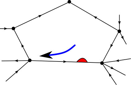 Figure 1
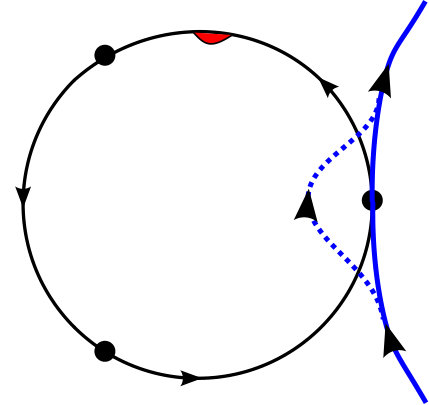 Figure 2
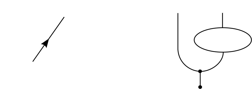 Figure 3
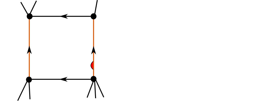 Figure 4
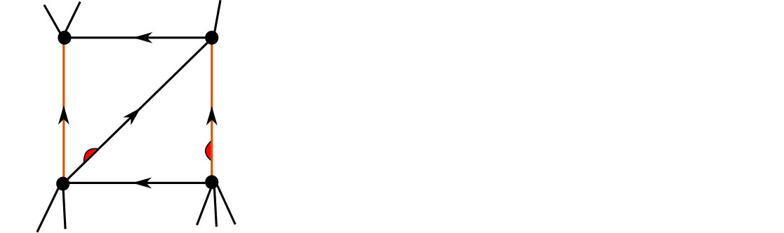 Figure 5
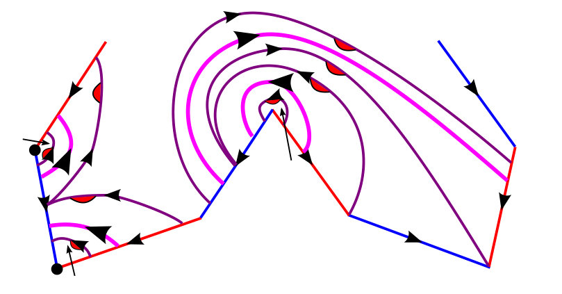 Figure 6
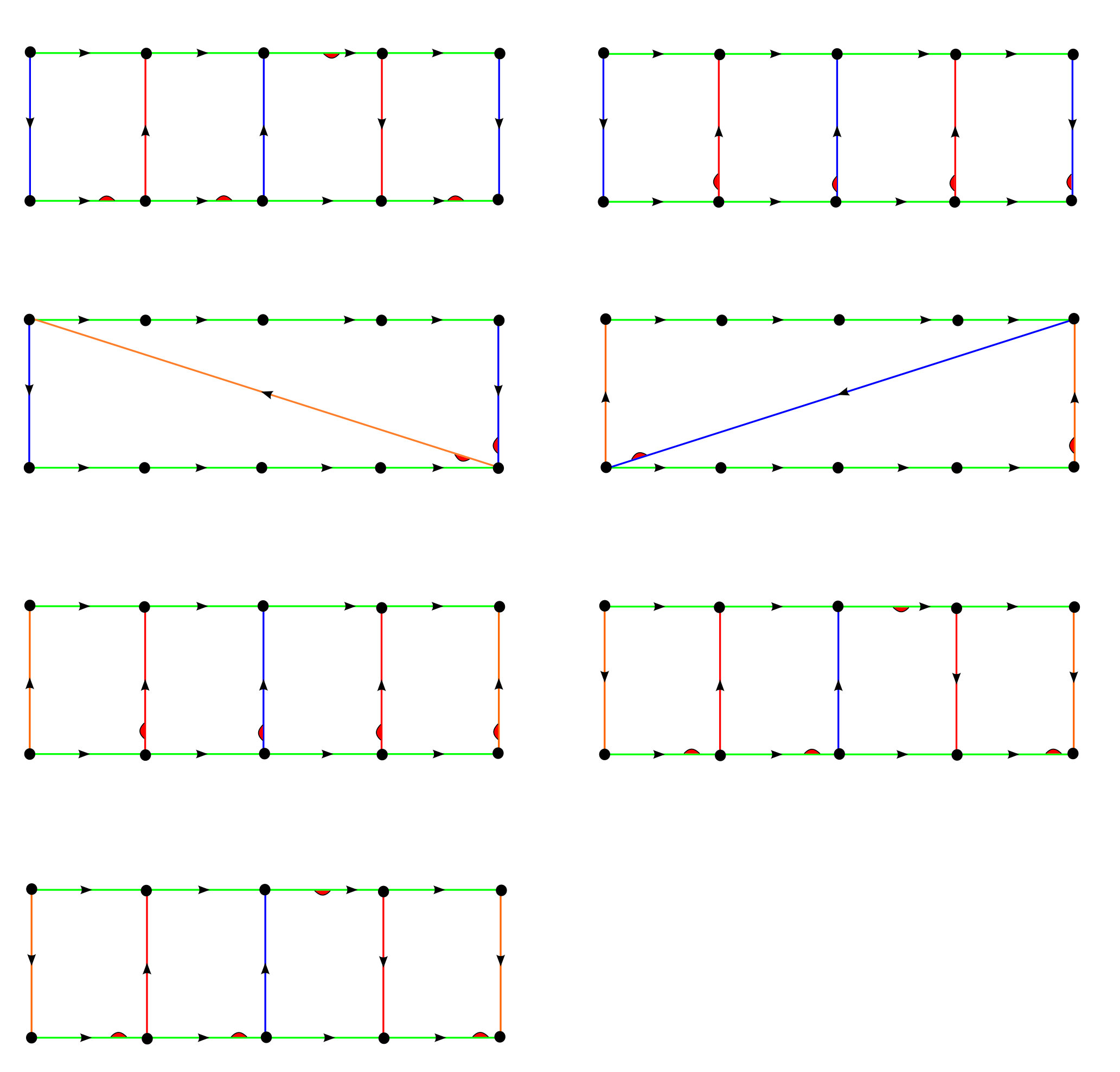 Figure 7
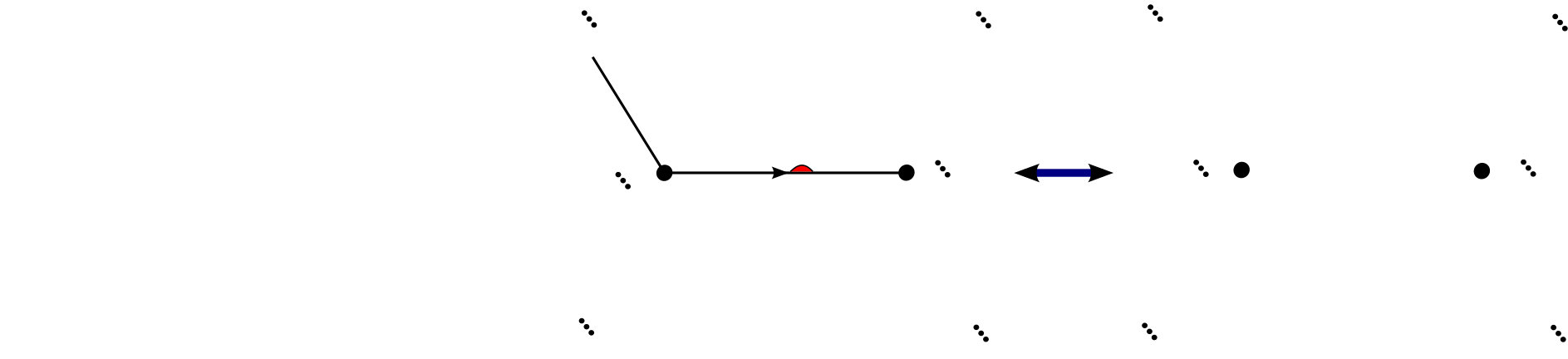 Figure 8
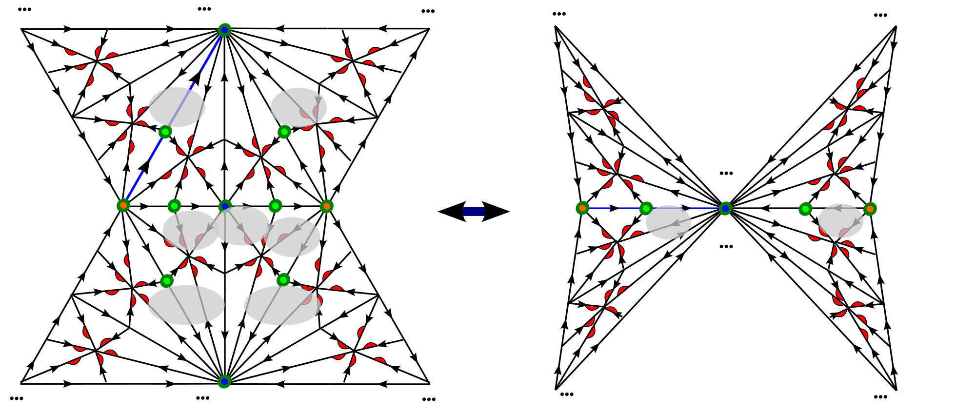 Figure 9
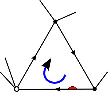 Figure 10
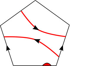 Figure 11
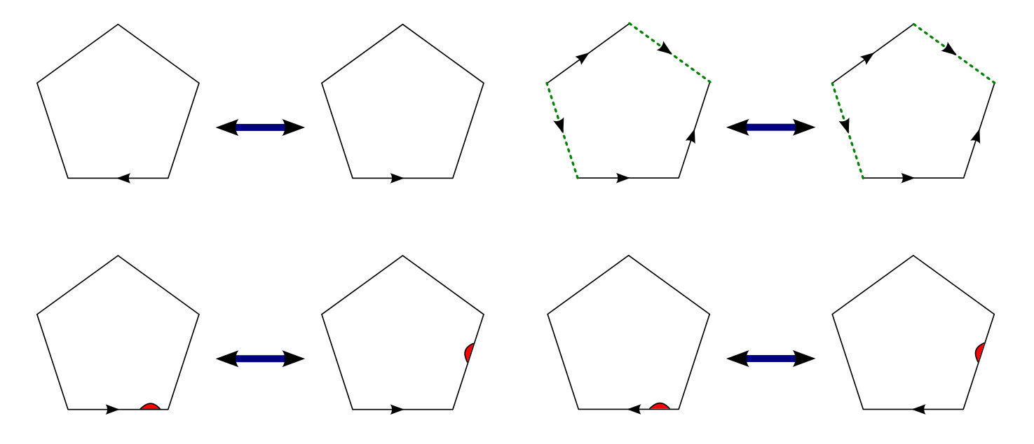 Figure 12
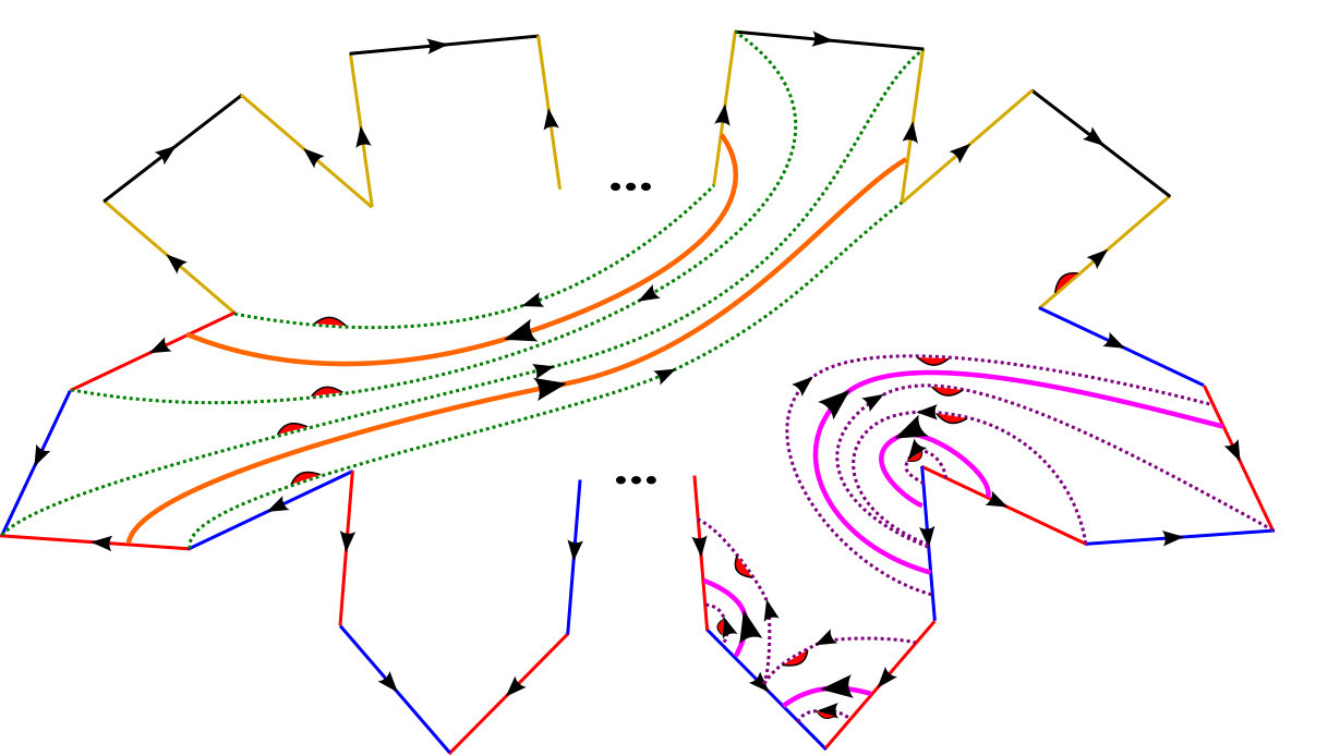 Figure 13
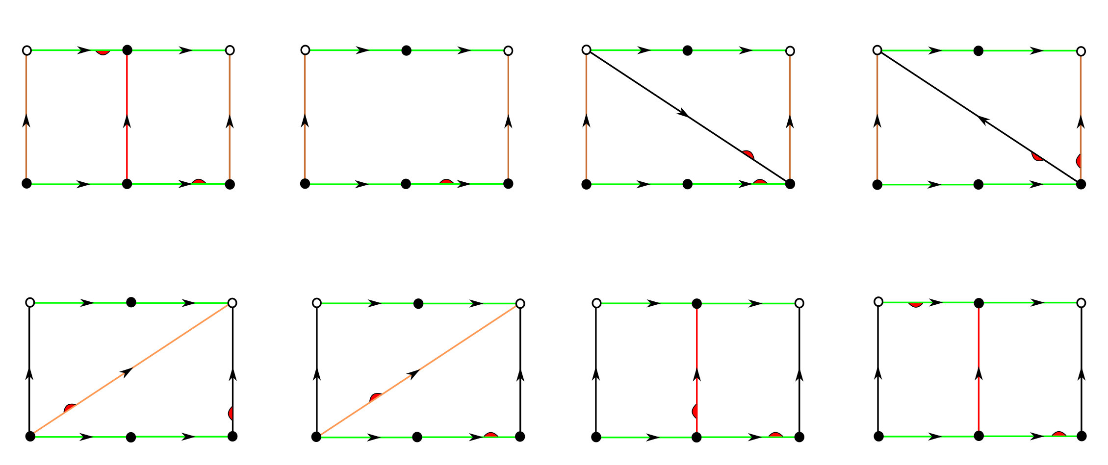 Figure 14
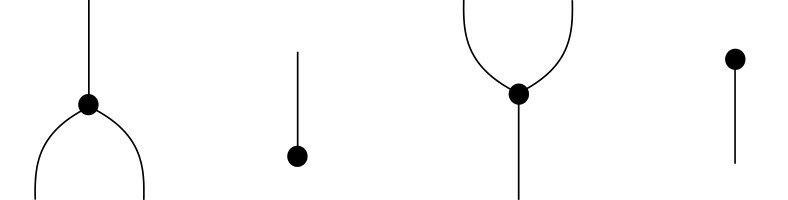 Figure 15
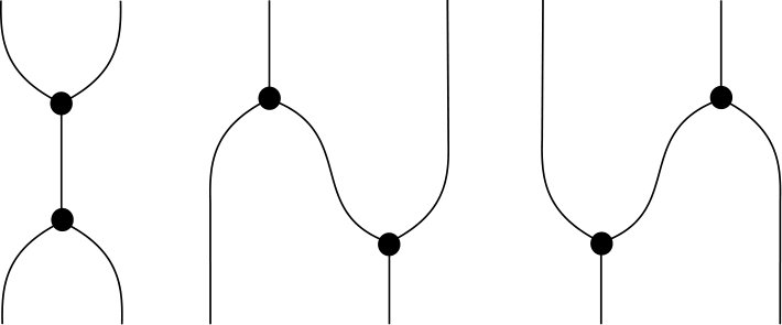 Figure 16
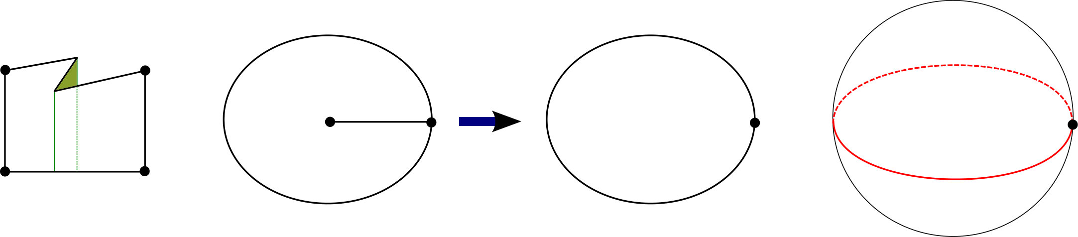 Figure 17
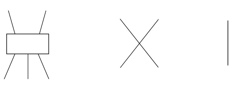 Figure 18
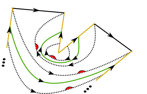 Figure 19
 Figure 20
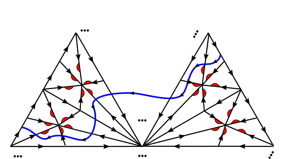 Figure 21
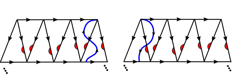 Figure 22
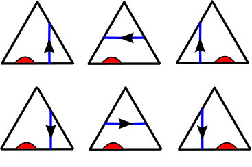 Figure 23
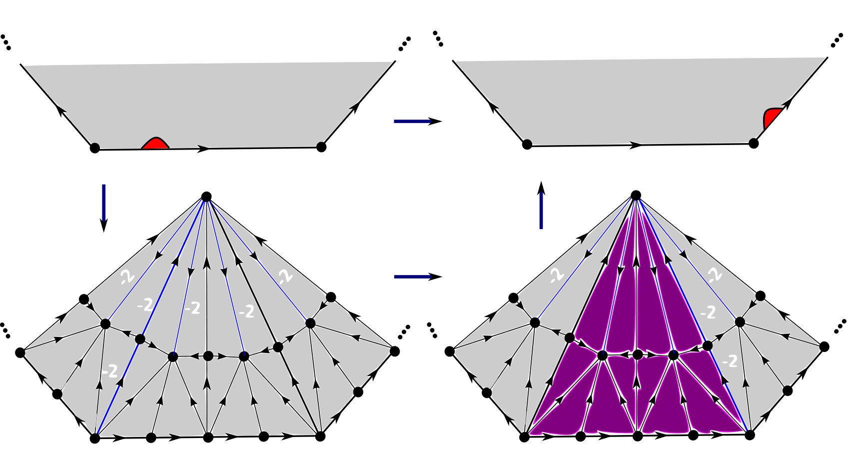 Figure 24
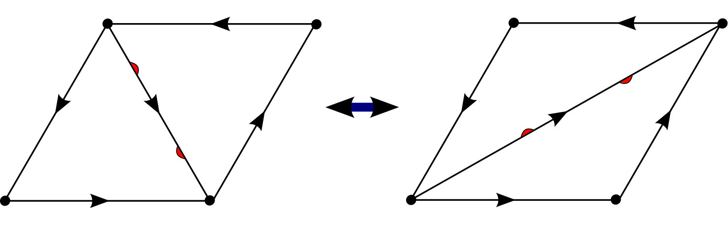 Figure 25
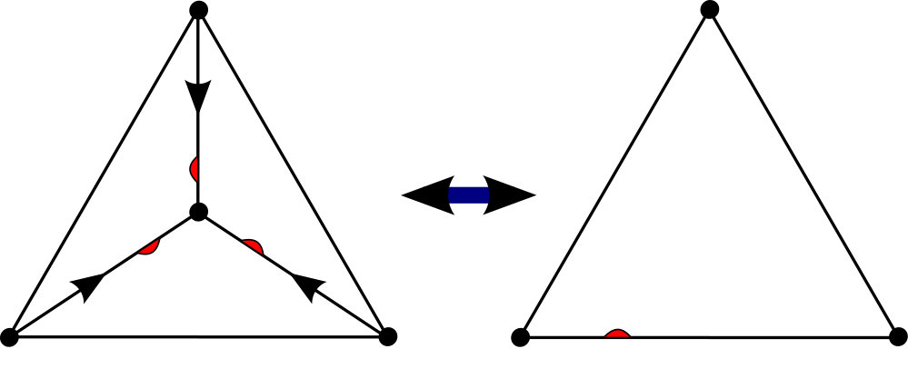 Figure 26
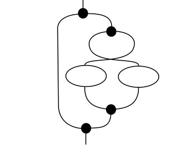 Figure 27
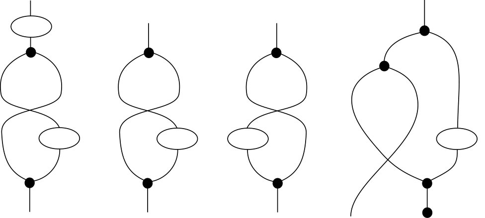 Figure 28
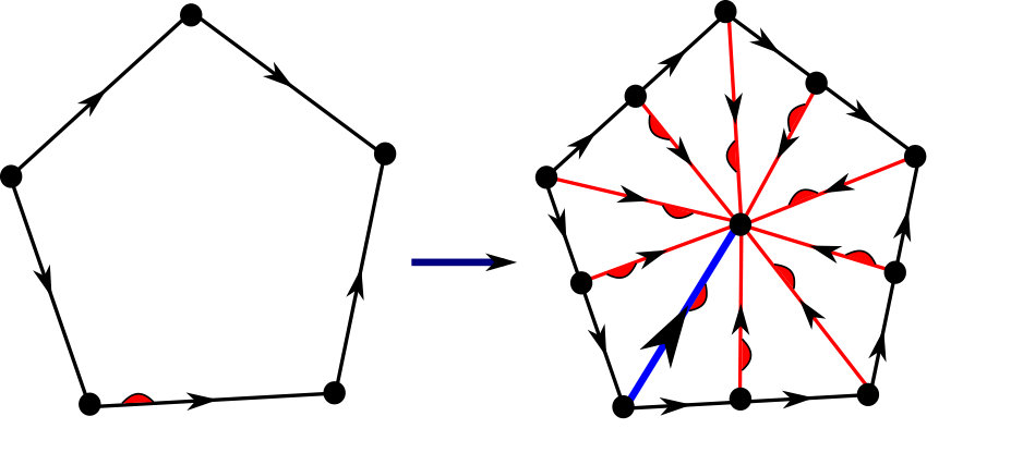 Figure 29
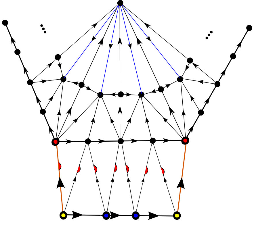 Figure 30
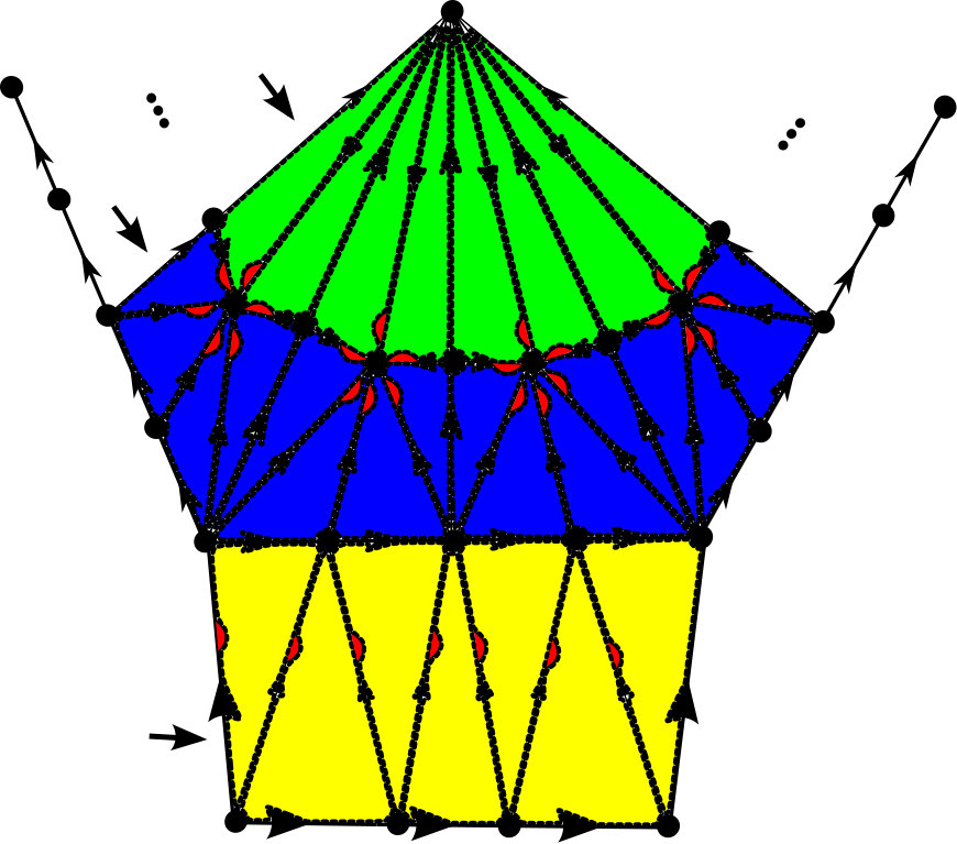 Figure 31
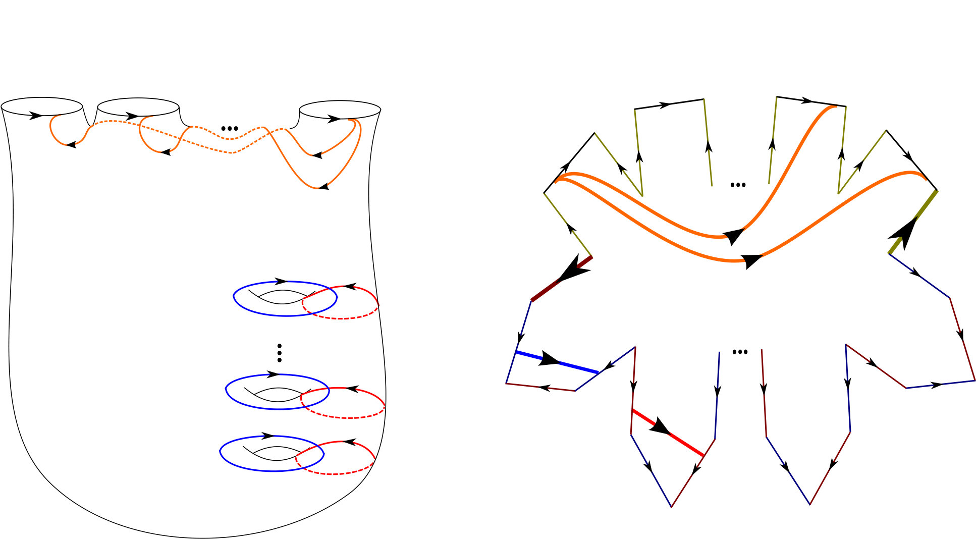 Figure 32
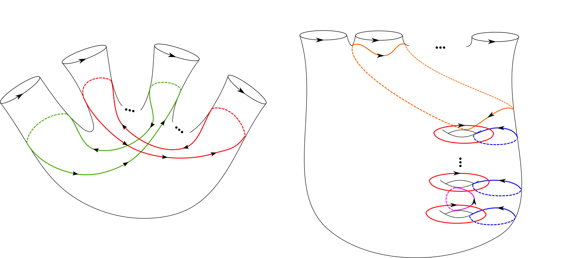 Figure 33
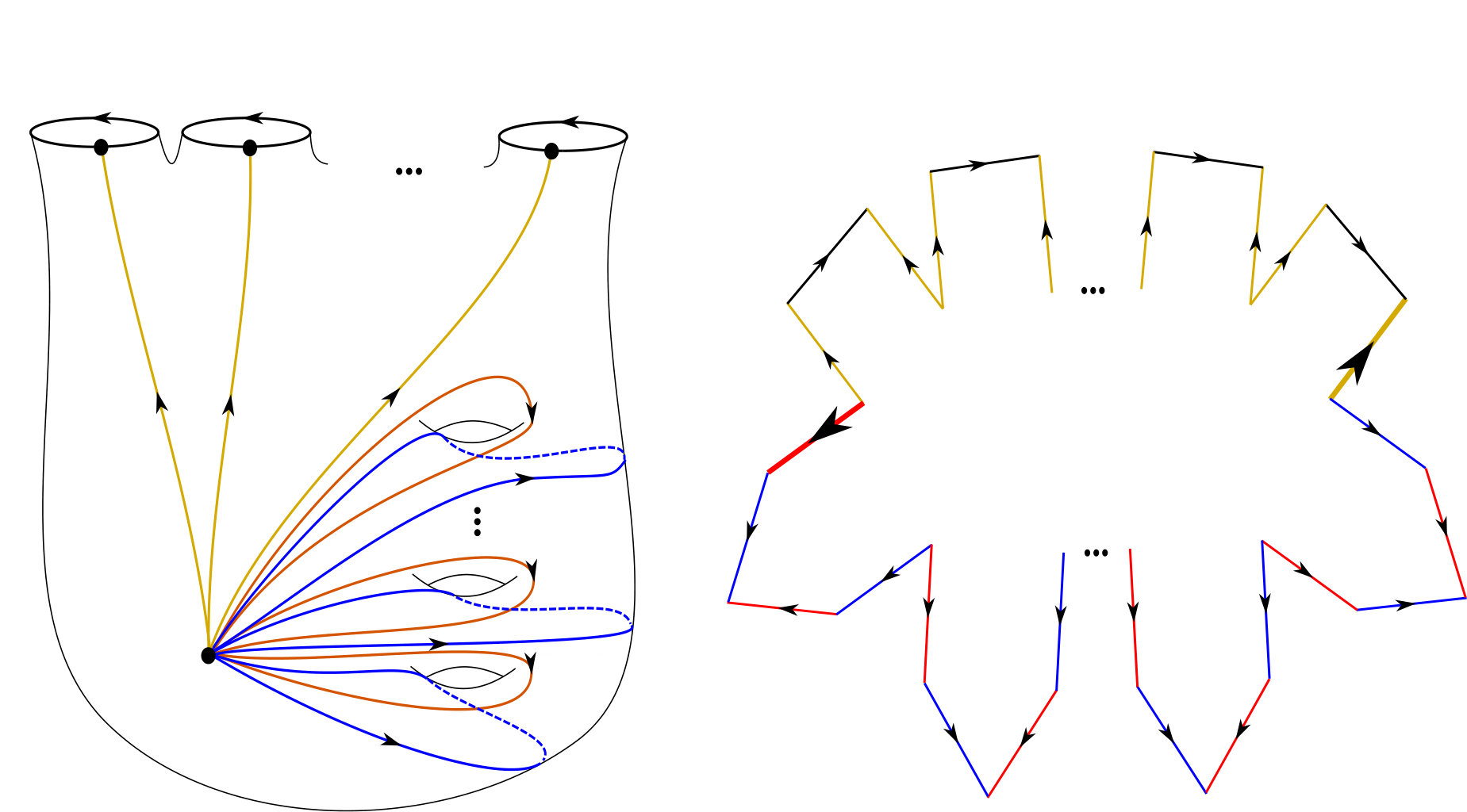 Figure 34
 Figure 35
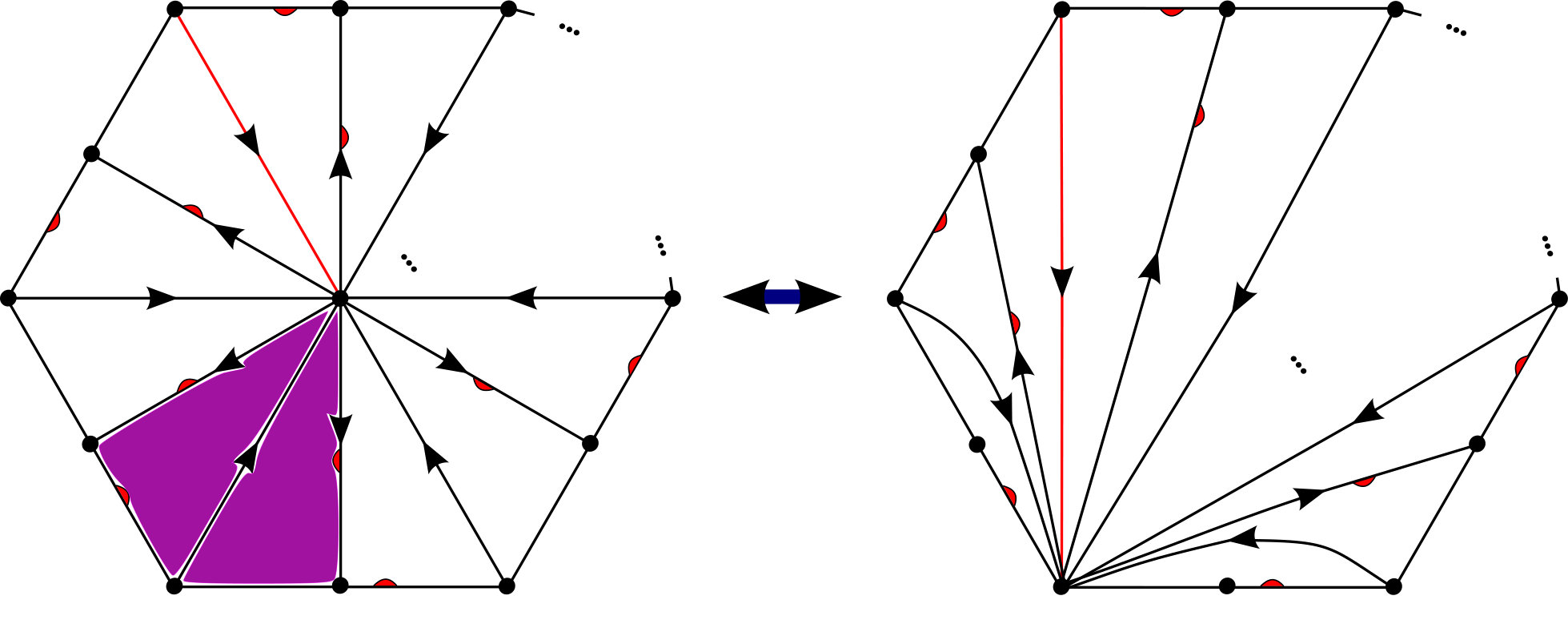 Figure 36
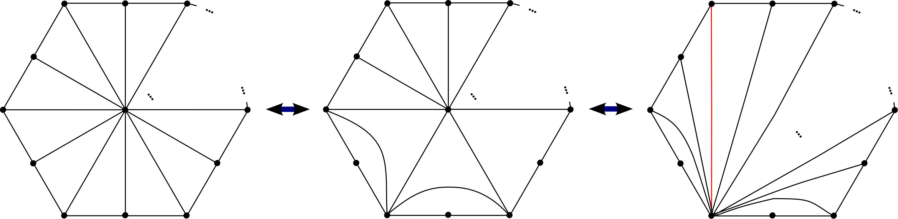 Figure 37
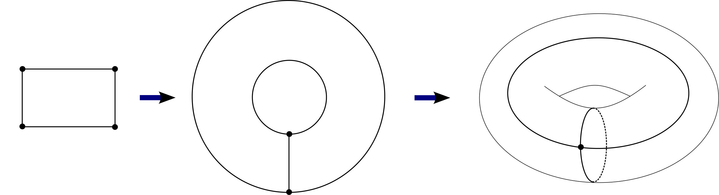 Figure 38
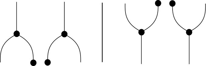 Figure 39
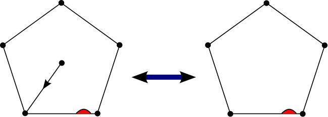 Figure 40
Peer Reviews
No public reviews on file for this paper yet. If you reviewed it on a platform where reviews are public (OpenReview, ICLR, NeurIPS, ICML), you can paste yours below so the community can read it here.
Videos
No videos yet. Explain this paper in a talk, walkthrough, or lecture? Add one.
Taxonomy
TopicsTopological and Geometric Data Analysis · Algebraic structures and combinatorial models · Theoretical and Computational Physics
\WarningFilter
latexText page \WarningFilterlatexReference
ZMP-HH/18-7
Hamburger Beiträge zur Mathematik 726
Topological field theory on -spin surfaces
and the Arf invariant
Ingo Runkel a and Lóránt Szegedy b ***Emails: [email protected] , [email protected]
a Fachbereich Mathematik, Universität Hamburg
Bundesstraße 55, 20146 Hamburg, Germany
b Institute of Science and Technology Austria
Am Campus 1, 3400 Klosterneuburg, Austria
Abstract
We give a combinatorial model for -spin surfaces with parametrised boundary based on [No]. The -spin structure is encoded in terms of -valued indices assigned to the edges of a polygonal decomposition. This combinatorial model is designed for our state sum construction of two-dimensional topological field theories on -spin surfaces. We show that an example of such a topological field theory computes the Arf-invariant of an -spin surface as introduced in [Ra, GG]. This implies in particular that the -spin Arf-invariant is constant on orbits of the mapping class group, providing an alternative proof of that fact.
Contents
1 Introduction
-spin topological field theories
The rotation group in two dimensions is fundamentally different from the higher dimensional rotation groups. Namely, for has universal cover which has a finite fibre (namely ), while the universal cover of is which has an infinite fibre given by . Accordingly, in two dimensions one can speak of -spin structures, for , where one considers the connected cover of with fibre . The special case is the universal cover. We review -spin surfaces in detail in Section 2.1. Here we only mention that a -spin surface is just an oriented surface, a -spin surface is what is usually referred to as a surface with spin structure, and giving a [math]-spin structure on a surface is equivalent to giving a framing. We stress that the case is included in all of the following discussion.
We consider -spin surfaces whose boundary components are parametrised by annuli with -spin structure. The -spin structures on these annuli are in bijection with . The -spin surfaces with parametrised boundary form a symmetric monoidal category , whose objects are “circles with -spin structures”, which we describe as finite lists of elements of , and which dictate the restriction of the -spin structure of a bordism to the in- and outgoing boundary components.
One defines a two-dimensional -spin topological field theory (TFT) to be a symmetric monoidal functor
[TABLE]
for a symmetric monoidal target category , which we will assume to be additive and idempotent-complete (and have countable direct sums in case ).
Combinatorial model of -spin surfaces
In [No] a combinatorial description of -spin surfaces is given based on the choice of a triangulation. For our applications, triangulations are cumbersome due to the large number of triangles required even for simple surfaces. We give a more convenient combinatorial model based on decompositions into polygons called PLCW-decompositions [Ki] (see Section 2.2). For example, this allows one to describe a genus -surface with boundary components with in terms of a single -gon with appropriately identified edges.
The combinatorial representation of an -spin structure on a surface is in terms of a marked PLCW-decomposition, that is:
- •
a PLCW decomposition of such that each boundary component contains a single edge and a single vertex,
- •
a choice of a marked edge for each face (before identification of the edges),
- •
an orientation of each edge,
- •
an edge index for each edge ,
and where the edge indices need to satisfy a consistency condition around each vertex, see Section 2.3. To obtain an -spin structure from the above data, one endows each face with its unique (up to isomorphism) -spin structure and then uses the edge indices to define transition functions between the faces. Finally, one extends the -spin structure to the vertices, which is possible due to the above consistency condition. Different sets of combinatorial data can describe isomorphic -spin structures on a given surface, and we give an equivalence relation which precisely encodes that redundancy (Theorem 2.13).
Remark 1.1**.**
The mapping class group of a surface acts on (isomorphism classes of) -spin structures on that surface. Counts of the orbits of this action can be found in several places in the literature [Ja, NP, Ra, GG, Ka, Sa]. They differ in the detailed setup and in the restrictions placed on . In [Sz] we give a different treatment covering all cases of using our combinatorial model and a state-sum -spin TFT.
State-sum construction
We use the above combinatorial model to give a state-sum construction of -spin TFTs. The input data is a Frobenius algebra whose Nakayama automorphism satisfies , and whose window element is invertible (here , , are the product, coproduct, and unit of , respectively). We have (Theorem 3.8):
Theorem 1.2**.**
Let be a Frobenius algebra with and with invertible window element in a symmetric monoidal category . The state-sum construction defines a symmetric monoidal functor
[TABLE]
We prove this theorem by reducing it to the case of state sums for triangulations, which was treated in [No]. State-sum constructions in the case of 2-spin were considered previously in [BT, NR, GK].
Write for the functor (1.1) obtained in this way. We show that
[TABLE]
where is the value of the functor on the -spin circle , gets equipped by with a unital associative -graded algebra structure which can be understood as a -graded version of the centre of an algebra (Proposition 3.10). For , this algebraic structure on state spaces has also been found in [MS].
In [DK] Frobenius algebras with appear under the name of -Frobenius algebras in relation to -spin surfaces. In [Sn] -Frobenius algebras have been used to describe -spin TFTs defined on “open bordisms”, meaning that the objects in the bordism category are disjoint unions of intervals. Our -spin TFTs are defined on “closed bordisms”, meaning that objects are disjoint unions of circles. These -spin TFTs have been classified in [SnSz] in terms of closed -Frobenius algebras.
TFT computing the Arf-invariant
As an example, let be the category of super vector spaces over some field not of characteristic and the Clifford algebra in one odd generator . Assume that is even. One finds that for and that the following holds (Section 4.1 and Theorem 4.6):
Theorem 1.3**.**
Let be an -spin surface of genus with ingoing boundary components of -spin structures and no outgoing boundary components. Then
[TABLE]
where is the Arf-invariant of the -spin structure of as defined in [Ra, GG].
By construction, is invariant under the action of the mapping class group of . Thus the above theorem also proves that the -spin Arf-invariant is constant on mapping class group orbits, a fact already shown in [Ra, GG] by different means. For usual spin structures, so , the fact that a spin-TFT can compute the Arf-invariant (incidentally, for the same algebra) was already noticed in [MS, Gu, BT, GK]. From this point of view Theorem 1.3 is not surprising as an -spin structure for even also defines a 2-spin structure, and this correspondence is compatible with the Arf-invariant. A slightly different notion of an Arf-invariant for -spin structures is given in [NP, Def. 5.1].
Structure of this paper
This paper is organised as follows. In Section 2 we describe the combinatorial model for -spin structures and state its main properties. In Section 3 we use this model to give a state-sum construction of -spin TFTs, and we compute the value of these TFTs on several bordisms as an example. In Section 4 we show that for even, the -spin state-sum TFT for the two-dimensional Clifford algebra computes the -spin Arf-invariant. Finally, in Appendix A we relate the description of -spin structures in terms of PLCW-decompositions that we use here to the triangulation-based model of [No]. We furthermore give the proofs of those properties of the combinatorial model and of -spin state-sum TFTs which require the triangulation-based model and have been omitted in the main text.
Acknowledgments
We would like to thank Nils Carqueville, Tobias Dyckerhoff, Jan Hesse, Ehud Meir, Sebastian Novak, Louis-Hadrien Robert, Nick Salter, Walker Stern and Lukas Woike for helpful discussions and comments. LS was supported by the DFG Research Training Group 1670 “Mathematics Inspired by String Theory and Quantum Field Theory”.
2 Combinatorial description of r-spin surfaces
In this section we present the combinatorial model for of -spin structures and state its properties. We start by reviewing the definition of an -spin structure (Section 2.1) and of the decomposition of surfaces we will use (Section 2.2). The main results in this section are the bijection of the combinatorial data modulo an appropriate equivalence relation and isomorphism classes of -spin structures (Theorem 2.13 in Section 2.3) and the counting of these isomorphism classes for compact connected surfaces (Proposition 2.21 in Section 2.6).
2.1 -spin surfaces
Here we recall the definition of -spin structures and of related notions, following [No]. Denote by the set of real matrices of positive determinant, and let be the -fold connected cover for and the universal cover for . Note that in both cases the fibres are isomorphic to . By a surface we mean an oriented two-dimensional smooth manifold. For a surface we denote by the oriented frame bundle over (“oriented” means that orientation on the tangent space induced by the frame agrees with that of ).
Definition 2.1**.**
An -spin structure on a surface is a pair , where is a principal -bundle and is a bundle map intertwining the - and -actions on and respectively. 2. 2.
An -spin surface is a surface together with an -spin structure. 3. 3.
A morphism of -spin surfaces is a bundle map between the -spin surfaces, such that the underlying map of surfaces is a local diffeomorphism, and such that the diagram
[TABLE]
commutes, where denotes the induced map from the derivative of . 4. 4.
A morphism of -spin structures over is a morphism of -spin surfaces whose underlying map of surfaces is the identity on . We write
[TABLE]
for the set of isomorphism classes of -spin structures on .
Note that is a -principal bundle (). Also, morphisms of -spin structures are always isomorphisms as they are maps of principal bundles. A diffeomorphism of -spin surfaces is a morphism of -spin surfaces with a diffeomorphism as underlying map of surfaces. Let us denote by
[TABLE]
the diffeomorphism classes of -spin surfaces with underlying surface . Note that by construction we have a surjection
[TABLE]
given by passing to orbits under the action of the mapping class group of acting on . As we shall see, this surjection is almost never injective.
Even though we do not need it in the rest of the paper, let us mention that a 0-spin structure is the same as a framing. A framing of is a homotopy class of trivialisations of the oriented frame bundle over . Let denote the set of framings of . We have:
Proposition 2.2**.**
There is a bijection .
Proof.
Take a framing and pick a representative trivialisation, i.e. an isomorphism of principal bundles . Define
[TABLE]
Then is a 0-spin structure. Changing by a homotopy gives an isomorphic 0-spin structure [Hu, Ch. 4, Thm. 9.9]. This defines a map .
Next we define a map in the opposite direction. Since is contractible, for any 0-spin structure , is a trivialisable principal bundle [Sd, Thm. 12.2]. Let denote such a trivialisation. Then there exists a unique morphism of principal bundles such that
[TABLE]
commutes. Again by contractability, any two choices of trivialisations are homotopic and so the corresponding are homotopic, too. By the same argument, different choices of representatives of isomorphism classes of [math]-spin structures give homotopic ’s. This defines a map .
The two maps and are inverse to each other. Indeed, for , the [math]-spin structure one obtains after constructing is isomorphic to via as in (2.6), so that indeed . Conversely, starting from a homotopy class of trivialisations , in computing we see that in (2.6) we can take and , so that . ∎
After this aside on framings, let us return to -spin surfaces and give a basic example which will later serve to parametrise the boundary components of -spin bordisms.
Example 2.3**.**
For let denote the -spin structure on given by the trivial principal -bundle and the map
[TABLE]
where acts on by
[TABLE]
Since the -action is from the right and is a group homomorphism, indeed intertwines the - and -actions.
Lemma 2.4** ([No, Sec. 3.4]).**
and are isomorphic -spin structures if and only if . The map , is a bijection.
In the case that , it will be convenient to fix once and for all a set of representatives of in , say , and to agree that for , stands for , with the chosen representative for .
Notations 2.5**.**
For an -spin surface , by abuse of notation we will often use the same symbol to denote its underlying surface. That is, stands for the triple from Definition 2.1 (1).
A collar is an open neighbourhood of in . An ingoing (resp. outgoing) collar is the intersection of a collar with the set (resp. ). A boundary parametrisation of a surface is:
A disjoint decomposition (the in- and outgoing boundary components). and/or are allowed to be empty. 2. 2.
A collection of ingoing collars , , and outgoing collars , , together with a pair of orientation preserving embeddings
[TABLE]
We require that for each , the restriction maps diffeomorphically to the connected component of , and analogously for .
An -spin boundary parametrisation of an -spin surface is:
A boundary parametrisation of the underlying surface as above; we use the same notation as in (2.9). 2. 2.
A pair of maps fixing the restriction of the -spin structure to the in- and outgoing boundary components
[TABLE] 3. 3.
A pair of morphisms of -spin surfaces which parametrise the in- and outgoing boundary components by collars with -spin structure,
[TABLE]
Here, is the restriction of to the ingoing collar , and analogously . The maps of surfaces underlying are required to be the maps in (2.9) from Part 1.
Note that by Lemma 2.4, the maps in part 2 are not extra data, but are uniquely determined by the -spin surface and the boundary parametrisation.
For diffeomorphisms between -spin surfaces with parametrised boundary we only require that they respect germs of the boundary parametrisation. In more detail, let be as in (2.11) and let
[TABLE]
be another -spin surface with boundary parametrisation. A diffeomorphism of -spin surfaces with boundary parametrisation is an -spin diffeomorphism subject to the following compatibility condition. Let be an ingoing boundary component of and let be its image under . We require that and that . Furthermore, there has to exist an ingoing collar contained in both and such that the diagram
[TABLE]
of -spin morphisms commutes. An analogous condition has to hold for each outgoing boundary component .
By an -spin object we mean a pair consisting of a finite set and a map , . Below we will construct a category whose objects are -spin objects, and whose morphisms are certain equivalence classes of -spin surfaces, which we turn to now.
Definition 2.6**.**
Let and be two -spin objects. An -spin bordism from to is a compact -spin surface with boundary parametrisation as in (2.11) together with bijections and such that
[TABLE]
commute. We will often abbreviate an -spin bordism from to as .
Given -spin bordisms and , the glued -spin bordism is defined as follows. Denote by the source of , i.e. . For every , the boundary component of is glued to the boundary component of using the -spin boundary parametrisations and . The diagrams in (2.14) ensure that the -spin structures on the corresponding collars are restrictions of the same -spin structure on .
Two -spin bordisms between the same -spin objects, are called equivalent if there is a diffeomorphism of -spin surfaces with boundary parametrisation such that with ,
[TABLE]
commute. Let and be equivalence classes of -spin bordisms. The composition is well defined, that is independent of the choice of representatives , of the classes to be glued. In the following we will by abuse of notation write the same symbol for an -spin bordism and its equivalence class .
Definition 2.7**.**
The category of -spin bordisms has -spin objects as objects and equivalence classes of -spin bordisms as morphisms.
is a symmetric monoidal category with tensor product on objects and morphisms given by disjoint union. The identities and the symmetric structure are given by -spin cylinders with appropriately parametrised boundary.
2.2 PLCW decompositions
In Section 2.3 we will use a cell decomposition to combinatorially encode -spin structures on surfaces, and in Section 3.3 we will use this description to build an -spin TFT. For explicit calculations it is helpful to keep the number of faces and edges to a minimum. The notion of a PLCW decomposition from [Ki], and which we review in this section, is well suited for such calculations. For example, there is a PLCW decomposition of a torus consisting of 1 face, 2 edges and 1 vertex, see Figure 1. For comparison, using simplicial sets would require at least 2 faces, 3 edges and 1 vertex; using simplicial complexes (i.e. triangulations, as in [No]) would require at least 14 faces, 21 edges and 7 vertices (see e.g. [Lu]).
Now we turn to the definitions following [Ki]. Let be a compact set, let denote its interior and let denote its boundary. Let denote the closed -ball, or rather a piece-wise linear (PL for short) version thereof. Then is the (PL-version of the) -sphere. A PL map is called a regular map if is injective. A compact subset is a generalised -cell (or simply cell), if and for a regular map , which we call a characteristic map of . A generalised cell decomposition is a finite collection of cells such that the interiors of cells do not intersect and the boundary of any cell is a union of cells. Examples are shown in Figure 1 and in Figure 2. We denote the -skeleton of by , which is the union of the set of -cells with , and we define the dimension of to be the highest integer for which the set of -cells is nonempty. We denote the set of boundaries of an -cell by . A regular cell map between generalised cell decompositions and is a piecewise linear map such that for every with characteristic map there is a cell for which is a characteristic map. An example of a regular cell map is shown in Figure 1, a non-example is shown in Figure 2 .
Definition 2.8**.**
A PLCW decomposition is a generalised cell decomposition of dimension such that if
- •
is a PLCW decomposition and
- •
for any -cell with characteristic map there is a PLCW decomposition of , such that is a regular cell map.
Examples of PLCW decompositions are shown in Figure 1, Figure 2 and . A generalised cell decomposition which is not a PLCW decomposition is shown in Figure 2 . Each PLCW decomposition can be related by a series of local elementary moves (cf. Section 2.5 below), and each PLCW decomposition can be refined to a simplicial complex [Ki, Thm. 6.3]. For more details see [Ki, Sec. 6–8].
From now on we specialise to 2 dimensional PLCW decompositions. Let be a compact surface with a PLCW decomposition , , . We call these sets faces, edges and vertices respectively; one can think of faces as -gons with . For , PLCW decompositions also allow for a decomposition of any compact connected surface of genus and with boundary components into a single face which is a -gon, see Section 2.6.
To apply PLCW decompositions to smooth manifolds, we can use that a PLCW decomposition can be refined to a simplicial complex, and that PL cell maps for a simplicial complex can be approximated by smooth maps, giving smooth manifolds [Mu, Sec. 10].
2.3 Combinatorial description of -spin structures
In this section we extend the combinatorial description of -spin structures in [No], which uses a triangulation of the underlying surface, to PLCW decompositions. We will only consider PLCW decompositions where the boundary components consist of a single vertex and a single edge. In the following section we explain how this combinatorial model relates to the description of -spin structures in terms of holonomies of curves.
Let be a surface with parametrised boundary, with a PLCW decomposition, with a marking of one edge of each face and an orientation of each edge. We do not require that the orientation of the boundary edges corresponds to the orientation of the boundary components, but we orient the faces according to the orientation of the surface. This induces an ordering of the edges of each face, the starting edge being the marked one, see Figure 3. By an edge index assignment we mean a map , .
Definition 2.9**.**
We call an assignment of edge markings, edge orientations and edge indices a marking of a PLCW decomposition and a PLCW decomposition together with a marking a marked PLCW decomposition.
For a vertex let be the number of faces whose marked edge has as its boundary vertex in clockwise direction (with respect to the orientation of the face), as shown in Figure 3. Let denote the edges whose boundary contain :
[TABLE]
The orientation of an edge gives a starting and an ending vertex, which might be the same. Let (resp. ) be the number of edges starting (resp. ending) at the vertex and let
[TABLE]
We note that an edge which starts and ends at contributes 1 to both and to . For every edge let
[TABLE]
Recall the maps and from (2.10), as well as our convention that we only consider PLCW decompositions with exactly one vertex and one edge on each boundary component. For a vertex on a boundary component let us write by slight abuse of notation for this boundary component and let
[TABLE]
We call a marking admissible with given maps and , if for every inner vertex and for every boundary vertex the following conditions are satisfied:
[TABLE]
For an arbitrary marking of a PLCW decomposition of one can define an -spin structure with -spin boundary parametrisation on minus its vertices by taking the trivial -spin structure on faces and fixing the transition functions using the marking. The marking of an edge for a face contains the information how a standard polygon is embedded into the surface. The above -spin structure extends uniquely to the vertices of , if and only if the marking is admissible for and . The -spin boundary parametrisations are given by the inclusion of -spin collars (as prescribed by and ) over the collars of the boundary parametrisation of . For more details on this construction we refer the reader to Appendix A.3.
Definition 2.10**.**
Denote the -spin structure with -spin boundary parametrisation defined above by .
There is some redundancy in the description of an -spin structure via a marking. A one-to-one correspondence between certain equivalence classes of markings and isomorphism classes of -spin structures will be given in Theorem 2.13 below. As preparation we first give a list of local modifications of the marking which lead to isomorphic -spin structures.
Lemma 2.11**.**
The following changes of the marking of the PLCW decomposition of (but keeping the PLCW decomposition fixed) give isomorphic -spin structures:
Flip the orientation of an edge and change its edge index (see Figure 4 (1)). 2. 2.
Move the marking on an edge of a polygon to the following edge counterclockwise and change the edge index of the previously marked edge , if this edge is oriented counterclockwise, otherwise (see Figure 4 () and ()). 3. 3.
Let . Shift the edge index of each edge of a polygon by , if the edge is oriented counterclockwise with respect to the orientation of the polygon, and by otherwise. If two edges of a polygon are identified (i.e. are given by the same ), do not change its edge index. For an illustration, see Figure 4 Part . We call this a deck transformation.
These operations on the marking commute with each other in the sense that the final edge indices do not depend on the order in which a given set of operations 1–3 is applied.
Note that the operation in 3 is the same as moving around the marking of a face completely by applying operation 2. This lemma is proved in Appendix A.4.
Let be a surface with a fixed PLCW decomposition. Write for a given marking of , where denotes the edge markings of the faces, the edge orientations and the edge indices (cf. Definition 2.9). Let denote the set of all admissible markings for the maps and on . The operations in Lemma 2.11 generate an equivalence relation on . Let us denote equivalence classes by . The following lemma gives a more concrete description of the equivalence classes.
Lemma 2.12**.**
Let . We have:
For every choice there is some such that . 2. 2.
For a given choice of edge indices we have if and only if and are related by a sequence of deck transformations (operation 3) in Lemma 2.11.
Proof.
The first statement is immediate from operations 1 and 2 in Lemma 2.11. For the second statement recall that operations 1–3 commute, and operation 3 is redundant. Any sequence of operations can thus be written as M=\prod_{e}(\text{op.\,\ref{lem:moves:1} for edge e})\prod_{f}(\text{op.\,\ref{lem:moves:2} for face f}). Since and do not change, operation 1 for an edge must occur in pairs, leaving unchanged, and operation 2 for a face must occur in multiples of the number of edges of that face, so that the total change is expressible in terms of operation 3, M=\prod_{f}(\text{op.\,\ref{lem:moves:3} for face f}). ∎
Let denote the isomorphism classes of -spin structures with -spin boundary parametrisation for the maps and . The following theorem is proved in Appendix A.4.
Theorem 2.13**.**
Let be a surface with PLCW decomposition. The map
[TABLE]
is a bijection. On the right hand side it is understood that the edge markings and orientations of are given by .
Remark 2.14**.**
When combined with Lemma 2.12, this shows that for a fixed edge marking and orientation the admissible edge index assignments up to deck transformations are in bijection with the isomorphism classes of -spin structures with -spin boundary parametrisation for the maps and .
2.4 Holonomies in the combinatorial model
In this section we explain how to compute holonomies along curves in which then characterise the -spin structure on . We hope that this sheds some light on the geometric meaning of the quantities appearing in the combinatorial model.
Let be a compact -spin surface with parametrised boundary with maps and . By a curve in we mean a smooth immersion (i.e. has nowhere vanishing derivative), and which is either closed, or which starts and ends on the boundary of . In the former case we require in addition that the tangent vectors at the start and end point agree: . In the latter case we require that the start and end points are the images of under the boundary parametrisation maps and that the tangent vector of the curve is the same as the tangent vector of the boundary curve. Two curves and with and are homotopic if there is a homotopy between them, such that for each , is a curve in the above sense. In particular, since must remain nonzero everywhere along the homotopy, one cannot “pull straight” a loop in the curve.
Pick a lift of to the oriented frame bundle by taking the tangent vector of (which is non-zero since is an immersion) and adding another non-zero and non-parallel vector such that the orientation induced by them agrees with the orientation of the surface. Such a lift of a curve in to is unique up to homotopy, see e.g. [No, p. 26]. Also, if two curves in are homotopic, then their lifts to are homotopic as well.
Consider a disc around in with -spin structure given by the restriction of for as in Example 2.3. As on a contractible surface, all -spin structures are isomorphic (see e.g. [No, Lem. 3.10]), there is an isomorphism of -spin structures . In fact, there are exactly such isomorphisms, and we pick the one which acts as the identity on the fibre over (by Example 2.3, the fibre and projection over agree for all ). This construction will be needed to assign a holonomy to curves between different boundary components.
Recall that is a principal bundle over . Pick a lift of to the -spin bundle. Since the fibers of are discrete, this lift is unique after fixing it at one point and homotopic curves in lift to homotopic curves in . If is a closed curve let denote the holonomy of at . If is not closed, use the isomorphism from above to identify the fibers over the start- and end-point of , and let again denote the resulting holonomy of .
We now explain how to compute these holonomies in terms of the combinatorial description of -spin structures. Take a decorated PLCW decomposition of with edge index assignment and consider the -spin structure given by Definition 2.10. We may assume the PLCW decomposition to be fine enough so that its edges split into a set of arcs as in Figure 5. Then for every there is a face containing and an edge in the boundary of where the arc leaves the face (see Figure 5). Let us assume that is not a boundary edge. For the edge index of the edge let if the edge and cross positively, and otherwise (see again Figure 5 for conventions). Let if the clockwise vertex of the marked edge of the face is on the right side of (before glueing the edges) and otherwise. If is not a closed curve, let (resp. ) denote the boundary edge where starts (resp. ends), and let (resp. ) be its edge index. Recall that at the starting (ending) point of the tangent vector of is parallel to the boundary edge. Set if the edge and the tangent vector point in the same direction and otherwise. Set if the edge and the tangent vector point in the same direction and otherwise.
The proof of the following proposition relies on the relation to triangulations introduced in Appendix A and is given in Appendix A.6.
Proposition 2.15**.**
Let be a curve in . Then:
If bounds a disc embedded in , if is oriented counter-clockwise around the boundary of and otherwise. 2. 2.
If is a curve homotopic to then ; 3. 3.
We have
[TABLE]
Note that in Part 3, in case the curve goes from boundary to boundary, the edge index of the boundary edge where the endpoint of the curve lies is included in the sum over .
Example 2.16**.**
The admissibility conditions for an inner vertex (2.20) express that the -spin structure near the vertex is the trivial -spin structure, i.e. the unique one extending from the surface to the vertex. Indeed, pick a curve oriented counter-clockwise around the vertex. By part 1 of Proposition 2.15, the holonomy is . To match (2.23) and (2.20), it remains to check that . This in turn follows since an edge that contributes to has and vice versa.
2.5 Elementary moves on marked PLCW decompositions
In Section 2.3 we defined the -spin structure in terms of a marked PLCW decomposition, and we explained how to change the marking while staying within a given isomorphism class of -spin structures. In this section we state how the marking needs to change when modifying the underlying PLCW decomposition by elementary moves in order to produce isomorphic -spin structures.
Definition 2.17**.**
An elementary move on a PLCW decomposition of a surface is either
- •
removing or adding a bivalent vertex as shown in Figure 6 ), or
- •
removing or adding an edge as shown in Figure 6 ).
By [Ki, Thm. 7.4], any two PLCW decompositions can be related by elementary moves. We prove the following proposition in Appendix A.4.
Proposition 2.18**.**
The elementary moves in Figure 6 induce isomorphisms of -spin structures.
The edge index of an edge with a univalent vertex is fixed by the orientation and the marking of the edge, in particular it is independent of the rest of the edge indices. In Lemma A.6 we will show that removing univalent vertices induces an isomorphism of -spin structures. For an illustration, see Figure 7.
2.6 Example: Connected -spin surfaces
In this section we illustrate how one can use the combinatorial formalism to count isomorphism classes of -spin structures. This recovers results obtained in [Ra, GG] using a different formalism.
Notations 2.19**.**
Whenever it does not cause confusion we will use the same symbols for edge labels and for edge indices. For example for we will simply write instead of .
Lemma 2.20**.**
There exists -spin structures on the sphere if and only if or . If there exists an -spin structure on the sphere then it is unique up to isomorphism.
Proof.
Let us consider the sphere decomposed into two 1-gons, one edge and one vertex as in Figure 2 , with edge index (cf. Notations 2.19). Let us collect the ingredients for the vertex condition (2.20). The edge starts and ends at the vertex, therefore from (2.18).
The number of in- and outgoing edges for is , cf. (2.17). The number of faces with in clockwise direction from their marked edge is , since the edge is marked for both faces. The vertex condition (2.20) then reads
[TABLE]
which holds if and only if or . The edge index can be set arbitrarily by operation 3 in Lemma 2.11, and together with Remark 2.14 we see that for any two values of the -spin structures on the sphere are isomorphic. ∎
Proposition 2.21**.**
Let be a connected surface of genus with boundary components and with maps and . There exists an -spin structure on if and only if
[TABLE]
where denotes the Euler characteristic and was defined in (2.19). If (2.24) holds, the number of isomorphism classes of -spin structures on is given by:
[TABLE]
A similar result has been obtained for the existence of -spin structures on closed hyperbolic orbifolds for in [GG, Thm. 3]. Note that in complex geometry, (2.24) (for and ) is just the condition for the existence of an -th root of the canonical line bundle (see e.g. [Wi]).
Proof.
The case has been discussed in Lemma 2.20, so we can assume . Decompose into a -gon consisting of inner edges, boundary edges, one inner vertex and boundary vertices , , as shown in Figure 8 and . Assign the edge indices , , and , where and . Mark the edge if or the edge if , see Figure 8 .
We now evaluate the admissibility condition at each vertex. For the boundary vertex there is the incoming inner edge and the boundary edge which starts and ends at the same vertex . Therefore by (2.18), relative to one has and . For either of the two above mentioned markings and , therefore we have
[TABLE]
Thus the are uniquely fixed by the boundary parametrisation to be for all .
For the inner vertex there are edges leaving the vertex and edges which start and end there. Therefore by (2.18), relative to one has and . and , and so
[TABLE]
Combining (2.25) and (2.26) one obtains (2.24).
By Remark 2.14, for a fixed marking and orientation, edge index assignments up to deck transformations are in bijection with -spin structures. From (2.25) and (2.26) every gives an admissible edge index assignment. A deck transformation on the face shifts the parameters simultaneously and leaves the and parameters fixed. By a simple counting we get the number of isomorphism classes of -spin structures. ∎
Corollary 2.22**.**
There is a unique -spin structure on the disk with boundary condition (ingoing boundary) or (outgoing boundary), and no -spin structure else.
Let from (2.19) and let us denote the -spin structure on given by the parameters for and from Figure 8 by
[TABLE]
(and recall from Notation 2.19 that the same symbols denote edges and the assigned edge indices).
Proposition 2.23**.**
The holonomies of the curves in shown in Figure 9 are
[TABLE]
for and .
Proof.
We only show the calculation of the latter two holonomies. Consider the single face shown in Figure 9 . The tangent vectors of the edge and the loop point in the same direction and the loop starts at this edge (), therefore ; the tangent vectors of the edge and the loop point in the same direction and the loop ends at this edge (), therefore ; the clockwise vertex determined by the marked edge of the face is on the right side of the curve so . Taking the sum of all these we get . The edge and the loop cross negatively and the clockwise vertex is on the right side of the loop, so we get . ∎
3 State-sum construction of -spin TFTs
Our first application of the combinatorial description of -spin structures is a state-sum construction of -spin TFTs, see [BT, NR, GK] for the -spin case and [No] for general . We generalise the construction in [No] from triangulations to PLCW-decompositions, which are much more convenient for explicit computations. In Sections 3.1 and 3.2 we present some algebraic preliminaries, and in Section 3.3 we explain how suitable Frobenius algebras produce an -spin TFT via a state-sum construction (Theorem 3.8). In Section 3.4 we compute the value of the state-sum TFT on connected -spin bordisms.
3.1 Algebraic notions
Let denote a strict symmetric monoidal category with tensor product , tensor unit and braiding . We use the graphical calculus as shown in Figure 10, and we will omit the labels for objects if they are understood, as e.g. in Figure 11.
An object together with morphisms (multiplication), (unit), (comultiplication) and (counit), see Figure 11, is a Frobenius algebra if the following relations hold:
These relations imply that a Frobenius algebra is in particular an associative algebra and coassociative coalgebra, see [Ko, Prop. 2.3.24]. For more details on the definition of algebras, coalgebras and Frobenius algebras in monoidal categories we refer to e.g. [FS].
For a Frobenius algebra we define the window element [LP] and the Nakayama automorphism , see Figure 12. Then is central (as follows from an easy calculation) and is a morphism of Frobenius algebras (see [FS] and [NR, Prop. 4.5]). is called symmetric if . It can be shown from a straightforward calculation that is symmetric if and only if .
Lemma 3.1**.**
Let be a Frobenius algebra with Nakayama automorphism . Then for every
Proof.
The first and second equations are proven in [No, Lem. 5.12]. The third equation follows from a direct calculation. ∎
A morphism is called invertible if there is a morphism such that . In this case we write instead of for the unique inverse.
Let , be a Frobenius algebra in with invertible window element and with Nakayama automorphism , such that (for this last condition is empty). A Frobenius algebra with is called a -Frobenius algebra in [DK, Prop. I.41]. Define
[TABLE]
We collect some properties of in the following lemma.
Lemma 3.2**.**
is an idempotent, and for any one has that:
[TABLE]
Proof.
That is an idempotent is a direct generalisation of [No, Lem. 5.12 (1)]. The additional removes the “bubble” . The identity (3.2) is immediate from the definition of in (3.1) and the fact that is an automorphism of Frobenius algebras. The first identity in (3.3) is a more general version of [No, Lem. 6.8] and the proof works along the same lines. To show the second identity in each of (3.3) and (3.4) just write out the definition of , and . For the first identity in (3.4) use (3.3) together with
[TABLE]
which follows from a direct calculation. ∎
3.2 The -graded center
Let be a Frobenius algebra with invertible window element. Let be furthermore additive (in particular, finite direct sums distribute over tensor products) and assume that the idempotents split in , i.e.
[TABLE]
for some object . For assume furthermore that has countably infinite direct sums which distribute over the tensor product. We can now define:
Definition 3.3**.**
Let . The -graded center of a Frobenius algebra with invertible window element and which satisfies is the direct sum
[TABLE]
This is a -graded object and we call the degree of .
Next we will endow with an algebra structure induced by . Write
[TABLE]
for the embeddings of the summands in (3.8) and for the induced projections which satisfy
[TABLE]
Lemma 3.2 suggests to define, for ,
[TABLE]
By the universal property of direct sums (which in the countably infinite case for still distribute over by our assumptions) there is a unique map
[TABLE]
which satisfies . Let us furthermore define
[TABLE]
The morphisms and are degree preserving. It is straightforward to verify that together with and becomes an associative unital -graded algebra in .
One can restrict the Nakayama automorphism of on the ’s by
[TABLE]
As in [No, Lem. 5.12/3] on verifies that
[TABLE]
Recall from the introduction that denotes the non-negative generator of the ideal . In particular, for we have . The product is in general not commutative, but a simple computation shows that its components satisfy:
[TABLE]
Let be the unique morphism such that for all . Combining the fact that is an automorphism of Frobenius algebras with the definition of and and using (3.2) shows that is an algebra automorphism. By (3.14) we have . We collect the above results in the following proposition.
Proposition 3.4**.**
Let be as in Definition 3.3. The -graded center of is an associative unital algebra via , and is equipped with the algebra automorphism satisfying . The algebra satisfies the commutativity conditions, for ,
[TABLE]
Corollary 3.5**.**
The component of is a subalgebra and is the centre of .
Frobenius algebra structure for
For the rest of this section let us assume that . Since now is finite, we can define the coproduct as the sum
[TABLE]
with component maps
[TABLE]
We define the counit
[TABLE]
The morphisms and have degree +2 and -2 respectively. Note that we inserted a multiplication with and its inverse in the definition of and . The reason for this is that we want these maps to match the structure maps calculated in Section 3.4 from the state-sum construction.
It is straightforward to see that altogether becomes a Frobenius algebra, just verify (LABEL:eq:unit_counit) and (LABEL:eq:frob_rel) restricted to individual summands of by using Lemma 3.2 to move projectors past structure maps of and by the properties of itself. Altogether we have:
Proposition 3.6**.**
Let be as in Definition 3.3. For , the graded center of together with , , , is a -graded Frobenius algebra. The morphisms and have degree 0, while has degree and has degree .
Remark 3.7**.**
The condition amounts to being a representation of the group . Instead of defining this in a general category, let be a field and let us assume that , the category of -linear representations of . Then the algebra is the full center of as defined in [Da], and is in particular a commutative algebra in , the monoidal center of . To see this one needs to check that has the form of the full center as given in [Da, Prop. 9.6], which has been done in (3.15).
Note, however, that unless or , the counit and the comultiplication are not degree preserving, i.e. is not a Frobenius algebra in with these structure maps. 2. 2.
For one still obtains for every a non-degeneracy condition, which we do not explain in detail.
3.3 State-sum construction
Let again and be a Frobenius algebra with invertible window element and with . In this section we define a symmetric monoidal functor , that is, a TFT on two-dimensional -spin bordisms.
Recall the direct sum decomposition of the -graded centre from Definition 3.3. We define the TFT on objects as follows: Let be an -spin object. Then
[TABLE]
To define on morphisms is more involved and will take up the remainder of this section. Let and be two -spin objects. Let be an -spin bordism with maps , . Choose a decorated PLCW decomposition , , of the surface with admissible edge index assignment such that the -spin structure with parametrised boundary from Definition 2.10 is isomorphic to the -spin structure of the -spin bordism . Recall that and denote the in- and outgoing boundary components respectively and that by our conventions they are in bijection with edges on the boundary.
For a face which is an -gon let us write , for the sides of , where denotes the marked edge of , and the labeling proceeds counter-clockwise with respect to the orientation of . We collect the sides of all faces into a set:
[TABLE]
We double the set of edges by considering , where “” and “” stand for left and right, respectively. Let be the subset of all (resp. ), which have a face attached on the left (resp. right) side, cf. Figure 13 . Thus for an inner edge the set contains both and , but for a boundary edge the set contains either or . By construction of and we obtain a bijection
[TABLE]
where is the ’th edge on the boundary of the face lying on the side of , counted counter-clockwise from the marked edge of .
For every vertex in the interior of or on an ingoing boundary component of choose a side of an edge for which . Let
[TABLE]
be the resulting function.
To define we proceed with the following steps.
Let us introduce the tensor products
[TABLE]
Every tensor factor is equal to , but the various superscripts will help us distinguish tensor factors in the source and target objects of the morphisms we define in the remaining steps. 2. 2.
For an edge we set
[TABLE]
cf. Figure 13. Define the linear map
[TABLE]
where it is understood that the tensor factors in are assigned as indicated in (3.25). 3. 3.
Note that since all tensor factors in are algebras, so is itself. For and write
[TABLE]
where maps to the tensor factor . Define as the following product in the -algebra :
[TABLE]
Finally, we let be the endomorphism of obtained by multiplying with ,
[TABLE] 4. 4.
Let and let denote the -fold product for . Assign to every face obtained from an -gon the morphism and take their tensor product:
[TABLE] 5. 5.
We will now put the above morphisms together to obtain a morphism . Denote by the permutation of tensor factors induced by ,
[TABLE]
Using this, we define
[TABLE] 6. 6.
Let and denote the permutation of tensor factors induced by the maps and respectively:
[TABLE]
Using these permutations and the embedding and projection maps , from (3.6) we construct the morphisms linking the action of on objects to the tensor products :
[TABLE]
We have now gathered all ingredients to define the action of on morphisms:
[TABLE]
Theorem 3.8**.**
Let be a Frobenius algebra with invertible window element and with .
The morphism defined in (3.38) is independent of the choice of the marked PLCW decomposition and the assignment . 2. 2.
The state-sum construction yields a symmetric monoidal functor whose action on objects and morphisms is given by (3.20) and (3.38), respectively.
The proof of this theorem works by reducing to the corresponding statement for triangulations and is given in Appendix A.5.
Remark 3.9**.**
The above construction yields a TFT on the category of closed -spin bordisms, where the complete boundary of the -spin bordisms is parametrised, so the parametrised boundary is a closed manifold. One can define a different -spin bordism category, called the open-closed -spin bordism category, where only a one dimensional submanifold of the boundary of -spin surfaces is parametrised. The subcategory of the latter generated by the open cup, the open pair of pants and their duals is called the open -spin bordism category. In [Sn] a TFT on open -spin bordisms was constructed using -Frobenius algebras [DK, Prop. I.41] which are Frobenius algebras whose Nakayama automorphism satisfies .
3.4 Evaluation of state-sum TFTs on generating -spin bordisms
In this section we apply the state-sum construction from Theorem 3.8 to pairs of pants and discs with -spin structure. On the one hand, these bordisms generate , and on the other hand, we will recover the algebra structure of the -graded center of in this way. Finally, we evaluate on a connected bordism of genus with only ingoing boundary components.
Pair of pants as multiplication
Consider the -spin 3-holed sphere parametrised as in Section 2.6 with 2 ingoing boundary components and 1 outgoing boundary component between -spin objects and with () and . Let , and . Then by (2.19) , and . Substituting these and in (2.24) gives
[TABLE]
Denote this -spin bordism by
[TABLE]
(cf. (2.27)). The sets , are (see Figure 8)
[TABLE]
where in (3.41) the isomorphism is given by the order of elements of as listed. We have one inner vertex and 3 boundary vertices , and , with placed on the outgoing boundary component. We set
[TABLE]
Following the steps of the state-sum construction we get:
For the various edge indices
[TABLE]
from (3.26). Recall from Notation 2.19 that the same symbols denote edges and the assigned edge indices. 2. 3.
For the inner vertex and the ingoing vertices we set
[TABLE]
from (3.28) according to the map in (3.42). 3. 4.
For the single 9-gon from (3.30). 4. 5.
The permutation is from (3.31) where we use the cycle notation for the permutation of tensor factors. After a calculation using associativity of the product and the last equation of (LABEL:eq:plem), the morphism in (3.33) is
[TABLE] 5. 6.
For the in- and outgoing boundary components we get and from (3.36) and (3.37), since the permutations induced by and from (3.34) and (3.35) are identities. Also note that , etc. Finally by composing with and as in (3.38) we obtain
[TABLE]
Observe that from (3.10).
Cup as unit
Consider a disk with outgoing boundary. By Corollary 2.22, we get a unique -spin structure for boundary parametrisation, namely . Note that the map is unique. Using the notation in (2.27) we write . with . However, since the -spin structure is actually independent of we may as well set . We have
[TABLE]
There is an inner vertex and an outgoing boundary vertex , and we set
[TABLE]
By the state-sum construction one has
For the 2 edges from (3.26). 2. 3.
For the inner vertex from (3.28). 3. 4.
For the single 3-gon from (3.30). 4. 5.
The permutation is from (3.31). Putting the above together according to (3.33) we get
[TABLE] 5. 6.
For the (empty) in- and outgoing boundary components we get and from (3.36) and (3.37). From (3.38) we finally get
[TABLE]
Observe that from (3.12).
Pair of pants as comultiplication
Consider a 3-holed sphere with the parametrisation as above, just with in- and outgoing boundary components exchanged, i.e. , stand for outgoing boundary components, for the ingoing etc. Then from (2.24) one has:
[TABLE]
Denote this -spin surface with parametrised boundary by
[TABLE]
(cf. (2.27)). The morphism in (3.33) assigned to it by the state-sum construction is
[TABLE]
and from (3.38) one obtains
[TABLE]
Observe that from (3.18). While the above morphism is defined also for , as was remarked in Section 3.2 one can sum these morphisms only in the case when , in which case one obtains (3.17).
Cap as counit
Consider an -spin disk with ingoing boundary. By Corollary 2.22, the boundary parametrisation has and the -spin structure is independent of the edge indices. Denote this -spin surface with parametrised boundary with , (cf. (2.27)), with . By the state-sum construction one has
[TABLE]
Observe that from (3.19).
We collect the above computations for evaluated on generators in the following proposition:
Proposition 3.10**.**
Let be a Frobenius algebra with invertible window element and with , and let be the -spin TFT defined in Theorem 3.8. The the -graded center is equal to with product and unit (restricted to the corresponding graded components) given by and , respectively. For , we obtain an equality of Frobenius algebras.
For , the above relation between state spaces and the -graded center was already observed in [MS].
Connected -spin bordisms
Finally, let us evaluate on a general connected -spin bordism with only ingoing boundary components, that is, on in the notation of (2.27). Write
Using the decomposition of from Figure 8 , a straightforward computation along the same lines as above gives the following proposition.
Proposition 3.11**.**
Let denote the -spin surface of Definition 2.10 with only ingoing boundary components. Then
[TABLE]
4 -spin TFT computing the Arf-invariant
In this section we give an example for the state-sum construction of -spin TFTs, namely for the two-dimensional Clifford algebra in super vector spaces, and we compute its value on connected -spin bordisms (Section 4.1). We then recall the definition of the Arf invariant for -spin surfaces and observe that the TFT obtained from the Clifford algebra computes this invariant (Section 4.2).
4.1 -spin TFT from a Clifford algebra
Let be even and let be a field not of characteristic . Let be the Clifford algebra with one odd generator , i.e. with . We turn into a Frobenius algebra via
[TABLE]
Lemma 4.1**.**
For the Frobenius algebra the following hold.
, hence has invertible window element. 2. 2.
The Nakayama automorphism is given by . 3. 3.
For , , hence . 4. 4.
The morphism from (LABEL:eq:tftphi) is given by .
Proof.
. Its inverse is . 2. 2.
in any Frobenius algebra. We calculate in steps:
[TABLE] 3. 3.
We calculate in steps according to (3.1):
[TABLE]
We see that if and have the same parity this is the identity, otherwise this is zero, i.e. is a projection onto . 4. 4.
We calculate in steps according to (LABEL:eq:tftphi):
[TABLE]
where at the last step we execute first the summation over for a fixed and notice that we either get 0 or 2.
∎
Let denote the TFT from Theorem 3.8 given by the Frobenius algebra and recall from Section 2.6 the -spin structure with parametrised boundary with only ingoing boundary components and where . By calculating (3.54) in Proposition 3.11 and using (2.24) we get the following proposition.
Proposition 4.2**.**
The value of the TFT is
[TABLE]
Corollary 4.3**.**
Assume that , or else that and at least one of the ’s is odd (by (2.24) in this case and at least two ’s are odd). Then the following map is surjective:
[TABLE]
Remark 4.4**.**
One can show, using a similar argument as in [No, Sec. 6.5], that for any choice of Frobenius algebra with invertible window element and with the TFT of Section 3.3 is independent of the -spin structure. The idea is that if there exists a symmetric Frobenius algebra structure on an algebra , then is independent of the -spin structure for every other Frobenius algebra structure on as well. 2. 2.
Let be a positive integer and let us consider the category of -graded -vector spaces . By using the correspondence between braided monoidal structures on and quadratic forms on [JS] (see [FRS, App. A] for a review) one can check that for odd there is only one symmetric monoidal structure on . For even there are two: the trivial one inherited from and the non-trivial one given by the super grading. 3. 3.
One may wonder whether taking with some choice of symmetric monoidal structure would yield more examples of -spin TFTs than what one can find with target or . Part 2 shows that this is not so: All symmetric monoidal structures on are inherited from or (and only from the former for odd). Thus all algebras as in Theorem 3.8 are also algebras in , respectively , with the same properties, and produce the same results in the state-sum construction.
4.2 The -spin Arf-invariant
Definition 4.5** ([Ra, Sec. 2.4] and [GG, Sec. 5]).**
Let be even. The -spin Arf-invariant of the -spin surface is
[TABLE]
Notice that for even, -spin structures naturally factorise through -spin structures. Therefore it makes sense to talk about the Arf-invariant of them, which was introduced for 2-spin structures [Jo]. A related description of -spin structures and of their Arf-invariant is given in [NP, Def. 5.1] in terms of so called -Arf functions, and in [Sa, Sec. 3.1] using the language of winding number functions of [HJ], both akin to the from above
is invariant under the action of the mapping class group of , which has been proven in [Ra, Prop. 2.8] and [GG, Lem. 7]. We provide a different proof of this result in the corollary to the following theorem.
Theorem 4.6**.**
The TFT computes the -spin Arf-invariant:
[TABLE]
Proof.
This is immediate from Proposition 4.2, Proposition 2.23 and Definition 4.5. ∎
Since the morphisms in are diffeomorphism classes of -spin bordisms (relative boundary), we get:
Corollary 4.7**.**
The -spin Arf invariant is constant on mapping class group orbits.
Appendix A From triangulations to PLCW decompositions
By a triangulation of a surface we mean a smooth simplicial complex for the surface such that each boundary component consists of 3 edges and 3 vertices. In [No] a combinatorial description of -spin surfaces was given using triangulations. The purpose of this appendix is to show how to obtain the combinatorial description of -spin surfaces using PLCW decomposition of Section 2 from triangulations.
A.1 -spin surfaces with triangulations
Let us summarise the results of [No]. More precisely let us look at the differences between that formalism and the formalism developed in Section 2.
Let be a marked triangulation of a surface with parametrised boundary, i.e. every edge has an orientation and an edge index and every face has a marked edge. Let us assume that all boundary components are ingoing and recall the notions of Section 2.3. Put an additional marking on one of the edges of each boundary component . The induced orientation of the boundary component gives a starting and ending vertex of this additionally marked edge, see Figure 14. For a boundary vertex let if it is an ending vertex for the additionally marked edge and otherwise. We furthermore assume that the orientation of boundary edges agrees with the induced orientation of the boundary components. The marking is called admissible for a given map , if the following hold for every inner vertex and every boundary vertex on a boundary component .
[TABLE]
Here, , and are defined as in Section 2.3. According to the construction in [No, Sec. 4.8] we proceed as follows:
- •
Define an -spin structure on minus edges and vertices by giving the interior of the faces the trivial -spin structure .
- •
Define transition functions for every edge via the edge indices to extend the above to minus vertices. Note that the transition functions are constant valued functions, since these are transition functions for the -bundle .
- •
There is a unique -spin structure extending to the vertices if and only if the edge index assignment is admissible. Extend the -spin structure to the vertices.
- •
The -spin boundary parametrisation map is the inclusion of the -spin collars according to the map . The inclusions map to the boundary vertex determined by the extra marking of the given boundary component.
A.2 Distinguishing in- and outgoing boundary components
The glueing of -spin surfaces with parametrised boundary is defined as follows. First for every we specify an -spin lift ( in [No, Eqn. (3.35)]) of the map given by an element . Take two boundary components with -spin structure on a neighbourhood of these components and . We can glue these boundary components along their -spin boundary parametrisation composed with .
To define outgoing boundary components we precompose the above boundary parametrisations with for outgoing boundary components. (For convenience we will choose , as different choices of can be seen as composition with different -spin cylinders.) Then one can glue -spin boundary components along in- and outgoing boundary parametrisations as described in Section 2.1. We now give more details on the construction.
Let be an -spin surface with ingoing -spin boundary parametrisation
[TABLE]
for a map which maps . In order to distinguish in- and outgoing boundary components we first fix two sets as in Section 2.1. Let be the map . We define maps and by and . For the in- and outgoing -spin boundary parametrisations we set
[TABLE]
respectively. The admissibility condition (A.2) needs to be changed since we are parametrising outgoing boundary components with instead of with . This means that for a vertex on an outgoing boundary component the factor needs to be instead of , since .
A.3 Refining PLCW decompositions of -spin surfaces
By a series of radial subdivisions we mean radially subdividing the 1-cells and then the 2-cells, see Figure 15. This means splitting each edge in two by adding a vertex, adding a vertex to the interior of each face and adding edges between this new vertex and all other vertices of this face. The following lemmas follow from straightforward calculations.
Lemma A.1**.**
Let be a PLCW decomposition obtained by a series of radial subdivisions from a PLCW decomposition with admissible marking. Assign to new edges the markings, orientations and edge labels as shown in Figure 15. The vertex conditions (A.1) and (A.2) are satisfied at the old and new vertices.
Since we assumed that every boundary component consists of a single vertex and a single edge, applying two series of radial subdivisions gives four vertices and four edges on each boundary component. In order to get a triangulation we will modify this refinement as follows.
Lemma A.2**.**
Let be a marked PLCW decomposition obtained by applying the steps in Lemma A.1 twice on another PLCW decomposition with admissible marking. Add 7 triangles at each boundary component and assign the marking to the new edges as shown in Figure 16 and put the extra markings on edges on boundary components so that the ending vertex is in Figure 16. Then the conditions (A.1) and (A.2) hold at old and new vertices.
Sketch of proof.
Let us assume that at each boundary component there are only two edges connecting to the single vertex: the boundary edge and another one coming from the interior of the surface. In such a situation the refinement is shown in Figure 16. The conditions (A.1) and (A.2) can be checked by hand at every vertex.
If there are boundary components where more edges connect to the boundary vertex from the interior in the original PLCW decomposition, checking the conditions (A.1) and (A.2) is similar, but we omit the figure here. ∎
We now have all the ingredients needed to define an -spin structure with -spin boundary parametrisation using the tools developed by [No]. We proceed as follows.
- •
Take a surface with parametrised boundary and a marked PLCW decomposition with some edge indices and maps and .
- •
Refine this marked PLCW decomposition as described in Lemma A.2. This is a triangulation by [Ki, Thm. 6.3].
The new marking obtained this way is admissible in the sense of [No] (i.e. (A.1) and (A.2) hold) if and only if the marking of the original PLCW decomposition is admissible in the sense of Section 2.3 (i.e. (2.20) and (2.21) hold).
Definition A.3**.**
Let denote the -spin structure on obtained by the above steps.
A.4 Proofs for Section 2
Proof of Lemma 2.11.
Operation 1 follows directly from part 2 of [No, Lem. 4.11].
For Operation 3 do a deck transformation [No, Part 1 of Lem. 4.11] on all triangles inside the polygon.
For Operation 2 first notice that moving the marking of a polygon to the next clockwise edge amounts to changing the edge indices as in Figure 17. This is done by a deck transformation on all filled triangles.
It is a straightforward calculation to show that these operations commute with each other. ∎
Proof of Theorem 2.13.
Let be a surface with PLCW decomposition. Let the same surface, but now with a triangulation as obtained by a two-fold series of radial subdivisions as in Section A.3. For clarity, in this proof we will write for the surface without decomposition underlying both and .
In [No, Sec. 4.8] the set of admissible markings for a fixed triangulation of with only ingoing boundary components and fixed map has been defined along with a similar equivalence relation as , which we denote by . [No, Thm. 4.18] gives the isomorphism from the quotient of this set by to the isomorphism classes of -spin structures. By a simple reparametrisation as in Section A.2 one obtains from this the set of admissible markings for in- and outgoing boundary components and the set of isomorphism classes of -spin structures with in- and outgoing boundary components . Thus we get a bijection
[TABLE]
Let us denote by the map that sends a marked PLCW decomposition to its refinement according to Section A.3. Since the generators of the equivalence relation are built up from generators of the equivalence relation (see the proof of Lemma 2.11 above), we get a well defined map
[TABLE]
By construction the composition of the maps (A.3) and (A.4) is the map (2.22) in the statement of the theorem. It therefore remains to show that is a bijection.
is surjective: Let be an admissible marking of . As a first step, use the relation to change the edge markings and orientations to the form prescribed in Section A.3, resulting in a marking . Next follow the algorithm described in Figure 18 to bring all edge indices of in the interior of faces of to the form shown in Figure 16. Denote the resulting marking by . Let be an interior edge of and let be the edges of which cover , and , , the three additional vertices on . The admissibility condition around , , implies that the edge indices on must all be equal. The same argument shows that edge indices on boundary components are all equal. This shows that lies in the image of .
is injective: Let such that , i.e. . Notice that Lemma 2.12 and Remark 2.14 apply to marked triangulations as well. This means that we can assume that the marked edges and the edge orientations agree ( and ) for the PLCW decomposition and the triangulation as well. Furthermore, and are related by a series of deck transformation on the triangulation: .
Write for a deck transformation by units on the triangle of the triangulation of . Deck transformations on different triangles commute, so we can write the sequence of deck transformations as . It is not hard to see that the identity requires the for all belonging to a given face of the PLCW-decomposition of to be equal. But this precisely means that can be written as a product of deck transformations on the PLCW-decomposition of , i.e. . ∎
In the following we are going to give some tools that relate different marked triangulations and marked PLCW decompositions which parametrise isomorphic -spin structures. First we recall [No, Prop. 4.19 and 4.20].
Lemma A.4**.**
Let and be two -spin surfaces with triangulation and with the same underlying surface related by a Pachner 3-1 or 2-2 move as in Figure 19 and 20. Then these two -spin structures are isomorphic.
We define the -moves for as in Figure 21, which takes a -gon glued together from triangles to a -gon glued together from triangles.
Lemma A.5**.**
The move induces an isomorphism of -spin structures.
Proof.
First we show that one can obtain the move on a triangulation without any marking by a series of Pachner moves by induction on . For do a Pachner 2-2 move and then a Pachner 3-1 move as in Figure 22. Now assume that the statement holds for and show for . First we do two Pachner 2-2 moves and then apply a move as in Figure 23 to get exactly the move.
Since the Pachner moves in Figures 19 and 20 only change the marking locally, it is enough to check how the marking can possibly change near the vertices that are touched by these moves. If one calculates (2.20) for these vertices before and after a move one sees that the marking can only change according to Figure 21. ∎
Lemma A.6**.**
Removing a univalent vertex (whose edge was not marked) induces an isomorphism of -spin structures.
Proof.
When we remove an edge from a PLCW decomposition we need to compare the associated triangulation with marking from Definition A.3 and then use the above defined moves to go from one to the other. The part of the triangulations that need to be transformed into one another together with the transformation steps are shown in Figure 24. ∎
Proof of Proposition 2.18.
Move in Figure 6 for : As in the proof of Lemma A.6 we need to compare the marked triangulations associated to the marked PLCW decompositions. The part of the triangulations that need to be transformed into one another together with the transformation steps are shown in Figure 25.
Since we did local moves which induce isomorphisms of -spin structures, it is enough to check how the edge indices will change at those vertices which have been touched by the above moves. These vertices are marked with a circle. Observe that at the vertices , and one does not get any condition on . The vertices , , and get identified with others.
Assume that the vertices and are distinct and that (). At these two vertices one obtains .
Move in Figure 6: When removing a bivalent vertex as in Figure 6 , a similar argument applies.
Move in Figure 6 for : Indeed, look at the original PLCW decomposition and assume that the vertices and are the same. Insert a bivalent vertex on the edge, remove one of the two new edges by the above and then the univalent vertex with its edge using Lemma A.6. Again, one obtains .
This completes the proof of the proposition. ∎
A.5 Proof of Theorem 3.8
For Part 1 a direct computation shows that the morphism assigned to a PLCW decomposition and the morphism assigned to the triangulation obtained by the refinement of the PLCW decomposition are the same. One needs to use that multiplication with the ’s in the state-sum construction amount to canceling the “bubbles” . Independence of the choice of the function follows from the fact that is a central element.
Next we check independence from the triangulation and from the choice of marking (for a given -spin structure). Let us assume that has ingoing and no outgoing boundary components. Let denote the morphism in assigned to using a triangulation by the state sum construction of [No]. Note that we get three tensor factors of for each boundary component, since each boundary component consists of three edges. Now we explain how to reduce to for each boundary component. Recall that we used the notation for the cyclic permutation of the first and third tensor factors. Composing with , we obtain the morphism in (3.38). To show this we use that the factors of remove the “bubbles” . If has outgoing boundary components, it is easy to see that composing with appropriate factors of maps of [No, Sec. 5.4] and again yields the morphism in (3.38). Independence of the details of the triangulation is shown in [No, Thm. 5.10]. This latter theorem also states that for isomorphic -spin surfaces and , so that the assignment is well defined on morphisms.
For Part 2 functoriality can now be seen easily from the above discussion and by using [No, Prop. 5.11], since the embeddings and projectors and compose to , which can be omitted due to [No, Prop. 5.13]. Monoidality and symmetry follow directly from the construction. This completes the proof of Theorem 3.8.
A.6 Proof of Proposition 2.15
Part 1 does not involve the marked PLCW decomposition and is shown in [No, Lem. 3.12].
Part 2 follows directly from the discussion in the main text: homotopic curves in (in the sense described in the beginning of Section 4.2) have homotopic lifts in and homotopic curves in have the same lifts in after fixing them at the same starting point.
For Part 3, we are going to calculate the holonomy by summing up the contributions for all arcs as in (2.23).
The contribution for can be computed as follows. Take the face which crosses and take its refinement to a triangulation as in Section A.3. Let us first assume that this face has only inner edges, as in Figure 26. Let be the edge where leaves the face . The contribution of can now be calculated by summing up for each triangle the “” contributions of [No, Section 4.7]. For a given triangle and edge , where the curve leaves , the contribution is by [No, (4.33)], where is given in Figure 27.
First the curve crosses 3 triangles, which give a contribution of
[TABLE]
Notice that when afterwards crossing the dotted area, the lift of the curve does not pick up any of contributions: for every group of 4 triangles the contribution is
[TABLE]
If the marked edge of the face is on the right side of with respect to the orientation of then the curve has crossed the corresponding edge with edge label -2 and the contribution is
[TABLE]
Finally the curve crosses 6 triangles, which give a contribution of
[TABLE]
This proves the formula (2.23) if is a closed curve.
If the curve starts and ends on the boundary of the surface then we take it into account as follows. The parts of the triangulation where starts and ends is shown in Figure 28.
As described in the main text we have -spin isomorphisms of some neighbourhoods of the starting and ending point of , both sending these two points to . Under these isomorphisms the neighbourhood of , together with a part of and the boundary edges is shown in Figure 29. This way we can handle as a closed curve and by Part 3 we can modify the curve by a homotopy as in Figure 29, so that it crosses the edges and .
We can now calculate the contribution of these crossed triangles as before. The curve first crosses the boundary triangle in Figure 29 picking up the contribution
[TABLE]
Then it crosses the two triangles in Figure 28 picking up the contribution
[TABLE]
After crossing inner edges finally it crosses the two triangles in Figure 28 , using Figure 29, picking up the contribution
[TABLE]
Summing up the above contributions, we get formula (2.23).
This completes the proof of Proposition 2.15.
The reference list from the paper itself. Each links out to its DOI / PubMed record.
- 1[1]
- 2[BT] J.W. Barrett and S.O.G. Tavares, Two-dimensional state sum models and spin structures . Comm. Math. Phys. 336 (2015) 63–100 [1312.7561 [math.QA]] . · doi ↗
- 3[Da] A. Davydov, Centre of an algebra . Adv. Math. 225 (2010) 319–348 [0908.1250 [math.CT]] . · doi ↗
- 4[DK] T. Dyckerhoff and M. Kapranov. Crossed simplicial groups and structured surfaces . In T. Pantev, C. Simpson, B. Toën, M. Vaquié, and G. Vezzosi, editors, Stacks and Categories in Geometry, Topology, and Algebra , volume 643 , AMS (2015) [1403.5799 [math.AT]] . · doi ↗
- 5[FRS] J. Fuchs, I. Runkel, and C. Schweigert, TFT construction of RCFT correlators: III: simple currents . Nucl. Phys. B 694 (2004) 277–353 [hep-th/0403157] . · doi ↗
- 6[FS] J. Fuchs and C. Stigner, On Frobenius algebras in rigid monoidal categories . Arab. J. Sci. Eng. 33-2C (2008) 175–191 [0901.4886 [math.CT]] .
- 7[GG] H. Geiges and J. Gonzalo, Generalised spin structures on 2-dimensional orbifolds . Osaka J. Math. 49 , 449–470 (2012). · doi ↗
- 8[GK] D. Gaiotto and A. Kapustin, Spin TQF Ts and fermionic phases of matter . Int. J. Mod. Phys. A 31 (2016) 1645044 [1505.05856 [cond-mat.str-el]] . · doi ↗