Dirac ocillator in the cosmic string spacetime in the context of gravity's rainbow
K. Bakke, H. Mota

TL;DR
This paper investigates how gravity's rainbow modifies the energy levels of the Dirac oscillator in cosmic string spacetime, revealing significant alterations compared to the standard case without rainbow effects.
Contribution
It introduces a novel analysis of the Dirac oscillator within the gravity's rainbow framework in cosmic string spacetime, deriving modified energy levels.
Findings
Energy levels are significantly altered by gravity's rainbow functions.
Comparison shows deviations from the standard Dirac oscillator energy spectrum.
Results are visualized and contrasted with the non-rainbow scenario.
Abstract
In this paper we consider the Dirac oscillator in the context of Doubly General Relativity or Gravity's Rainbow. In order to obtain the energy levels of the Dirac oscillator, we solve the Dirac equation in the cosmic string spacetime modified by gravity's rainbow scenarios described by two rainbow functions. We then obtain that, as a consequence of the modification of the cosmic string line element by the two rainbow functions, the energy levels of the Dirac oscillator are appreciable altered. The results are plotted and compared with the standard case, without gravity's rainbow effects.
Click any figure to enlarge with its caption.
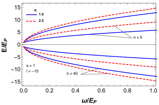 Figure 1
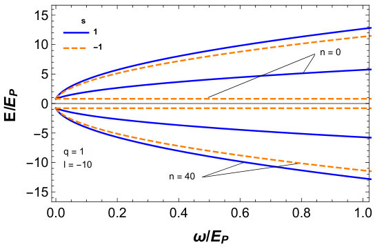 Figure 2
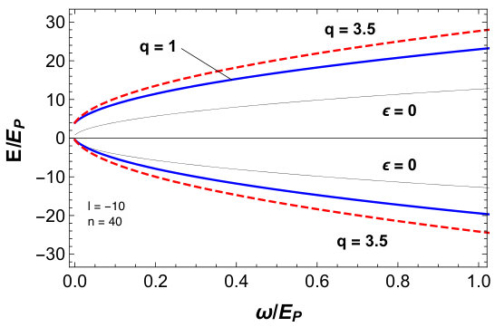 Figure 3
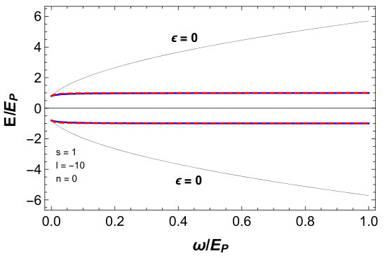 Figure 4
Peer Reviews
No public reviews on file for this paper yet. If you reviewed it on a platform where reviews are public (OpenReview, ICLR, NeurIPS, ICML), you can paste yours below so the community can read it here.
Videos
No videos yet. Explain this paper in a talk, walkthrough, or lecture? Add one.
Dirac ocillator in the cosmic string spacetime in the context of gravity’s rainbow
K. Bakke
Departamento de Física, Universidade Federal da Paraíba, Caixa Postal 5008, 58051-900, João Pessoa, PB, Brazil.
H. Mota
Departamento de Física, Universidade Federal da Paraíba, Caixa Postal 5008, 58051-900, João Pessoa, PB, Brazil.
Abstract
In this paper we consider the Dirac oscillator in the context of Doubly General Relativity or Gravity’s Rainbow. In order to obtain the energy levels of the Dirac oscillator, we solve the Dirac equation in the cosmic string spacetime modified by gravity’s rainbow scenarios described by two rainbow functions. We then obtain that, as a consequence of the modification of the cosmic string line element by the two rainbow functions, the energy levels of the Dirac oscillator are appreciable altered. The results are plotted and compared with the standard case, without gravity’s rainbow effects.
I Introduction
Semi-classical approaches to investigate quantum gravity phenomena are enormously useful, and any achievement coming from those should be expected to be present in the not yet known fully-fledged theory of quantum gravity. In this sense, an interesting phenomenological framework to study quantum gravity effects is the one of Doubly General Relativity or, as it is mostly known, Gravity’s Rainbow Magueijo:2002am ; Magueijo:2002xx ; AmelinoCamelia:2008qg . In this framework, the definition of a nontrivial dual space, as a consequence of a nonlinear Lorentz transformation in momentum space, implies that the metric describing the spacetime should be energy-dependent, leading to a modification of the relativistic dispersion relation. This energy is due to the particle(s) which ultimately probes the spacetime since for each value of the particle frequency it feels a different geometry.
In the context of Gravity’s Rainbow, there are in fact two quantities which are observer-independent (invariant): the speed of light and the Planck length (energy) AmelinoCamelia:2000mn ; Magueijo:2001cr ; Galan:2004st . Therefore, at high-energy scales (of the order of the Planck scale) the relativistic dispersion relation should acquire corrections Jacob:2010vr ; AmelinoCamelia:1997gz . This is in accordance, for instance, with ultra-high energy cosmic rays and TeV photons phenomena detected in experiments, suggesting the need of a modification of the relativistic dispersion relation AmelinoCamelia:1997gz ; Magueijo:2002xx ; AmelinoCamelia:2000mn ; AmelinoCamelia:2008qg .
The semi-classical approach of Gravity’s Rainbow has been used, for instance, to investigate Cosmological and Astrophysical phenomena in a variety of contexts ranging from Friedmann-Robertson-Walker Universe Khodadi:2016bcx ; Awad:2013nxa ; Majumder:2013ypa ; Hendi:2017vgo , black hole thermodynamics Hendi:2016dmh ; Hendi:2015cra ; Hendi:2015bba ; Hendi:2016vux ; Hendi:2016njy to neutron stars’ properties Hendi:2015vta , massive scalar field in the Schwarzschild metric Leiva:2008fd ; Li:2008gs ; Bezerra:2017hrb and Casimir effect Bezerra:2017zqq . These works show us a growing interest in the semi-classical approach of Rainbow’s Gravity as to investigate quantum gravity effects through corrections to the dispersion relation of relativistic quantum fields. Hence, in this work, we raise a discussion within the context of gravity’s rainbow by means of the effects that stem from high-order corrections to the relativistic dispersion relation of the Dirac oscillator in the cosmic string spacetime. The Dirac oscillator Moshinsky ; Villalba:1993fq is a relativistic model for the well-known harmonic oscillator Landau ; Griffiths , which is characterized by a coupling that keeps the Dirac equation being linear in both spatial coordinates and momenta. Besides, in the nonrelativistic limit of the Dirac equation, it recovers the spectrum of energy of the harmonic oscillator with a strong spin-orbit coupling. It has inspired a great deal of work Rozmej:1999jv ; Boumali2013 ; Quesne:2004pp ; 2008PhRvA..77c3832B ; Karwowski2007 ; Mandal:2009we ; PhysRevA.84.032109 ; Bakke:2013wla ; Bakke:2012zz ; Bakke:2013sla ; Bakke:2011qr ; Hassanabadi:2015hxa . Therefore, our interest is to extend the discussion about the semi-classical approach of gravity’s by analysing the influence of backgrounds determined by gravity’s rainbow on the spectrum of energy of the Dirac oscillator.
The structure of this paper is: in Sec.2 we introduce the cosmic string spacetime and the essential aspects of gravity’s rainbow framework that will modify the spacetime considered. Next, we solve the Dirac equation in the modified cosmic string spacetime, obtain the energy levels in two gravity’s rainbow scenarios presented and discuss the results comparing it with the results for the energy levels of the Dirac oscillator without gravity’s rainbow considered previously. Finally, in Sec.3 we present the conclusions. Throughout the paper we use natural units
II Dirac equation in the cosmic string gravity’s rainbow
In this section, we study the behaviour of the Dirac oscillator in two gravity’s rainbow scenarios, which we shall specify latter. Firstly, we start by introducing the spacetime background that we wish to work with, namely, the cosmic string spacetime described by the following line element VS ; hindmarsh :
[TABLE]
where the parameter is related to the deficit angle which is defined as , with being the linear mass density of the cosmic string. In the cosmic string spacetime, we have that Katanaev:1992kh ; Furtado:1994nq . Furthermore, in the cylindrical symmetry we have that , and . Cosmic string is a topological defect characterized by a spacetime with a conical topology and may have been produced by phase transitions in the early universe as it is predicted in extensions of the Standard Model of Particle Physics VS ; hindmarsh . Cosmic strings are also predicted in the framework of String Theory Hindmarsh:2011qj . Once formed, cosmic strings can evolve in the Universe and contribute to a variety of astrophysical, cosmological and gravitational phenomena VS ; hindmarsh ; escidoc:153364 ; Mota:2014uka , making the physics associated to them being of great relevance.
Let us now consider the framework of gravity’s rainbow. In the latter, as it has been said previously, the high-energy scale regime dictates that the relativistic dispersion relation, associated with a given quantum field of mass and momentum , has to be modified according to Magueijo:2002am ; Magueijo:2002xx ; Bezerra:2017zqq
[TABLE]
The functions and are called rainbow functions and their argument, , is the ratio of the energy of the probe particle to the Planck energy . This ratio regulates the level of the mutual relation between the spacetime background and the probe particles. Therefore, at low-energy regimes we must have
[TABLE]
It should be mentioned that it is possible to get gravity’s rainbow scenarios from theories with non-commutative geometries or other theories for quantum gravity such as loop quantum gravity Ashour:2016cay ; 2016arXiv160806824F ; Alsaleh:2017oae . It means that the rainbow functions can also be derived from these theories.
In the context of gravity’s rainbow, the line element of the cosmic string (1) becomes
[TABLE]
This modification of the cosmic string spacetime by gravity’s rainbow has been analysed previously in Ref. Momeni:2017cvl .
In the next (sub-)section we shall consider the Dirac oscillator in the background described by the line element (4) in order to see how the resulting energy levels associated with it get modified by the considered rainbow functions. They should be a generalization of the energy levels associated with the Dirac oscillator obtained in the background given by the line element (1). As it is known Bakke:2013wla , the energy levels of the Dirac oscillator obtained in the background of the cosmic string are given by the expression
[TABLE]
where is the frequency of the Dirac oscillator, is the mass and is the set of quantum numbers which take the values: , and . The parameter is given by
[TABLE]
Therefore, we can see that the energy levels above depends not only on the quantum numbers, mass, frequency but also on the cosmic string spacetime parameter . In the limit , one recovers the Dirac oscillator in Minkowski spacetime Bakke:2013wla .
The expression in Eq. (5) is plotted in Fig.1, in units of the Planck energy, in terms of the ratio of the Dirac oscillator frequency to the Planck energy. For both plots we consider . The scale in which these energy levels are plotted is more appropriate for latter comparison with the ones from gravity’s rainbow scenarios. On the left, the plot shows symmetric curves for values of the parameters indicated in the figure. The two internal curves (solid-blue and dashed-red) are for while the two external ones (solid-blue and dashed-red) are for . It is clear that if we decrease the cosmic string parameter , the positive and negative energies increase and decrease, respectively. On the other hand, the plot on the right shows symmetric curves for other set of parameter values as indicated in the figure. The dashed-orange and solid-blue curves are for different values of the spin, . We can see that, for the same values of the energy gets bigger or smaller depending on whether we take or , respectively. One could take different values for the quantum numbers and but this would only increase or decrease the energy, keeping the same shape for the graph. Note that although the plots may lead the reader to believe that the energy levels go to zero when the frequency goes also to zero, that is not true. In fact, the energy gets a nonzero values when .
II.1 First scenario of gravity’s rainbow
Let us now construct a scenario of the cosmic string gravity’s rainbow by using the following rainbow functions Bezerra:2017zqq ; Khodadi:2016bcx ; Awad:2013nxa ; Hendi:2017vgo :
[TABLE]
where we shall consider a first order parameter for our purposes. These rainbow functions fit the requirement of a constant velocity of light and solves the horizon problem puzzle Bezerra:2017zqq ; Khodadi:2016bcx ; Awad:2013nxa ; Hendi:2017vgo . In this first scenario of gravity’s rainbow, described by the rainbow functions in Eq. (7), the cosmic string line element (1) is modified according to (4) as
[TABLE]
Thus, we can note that by taking we recover the cosmic string line element (1), as it should be.
We can go further by using the spinor theory in curved space birrell1984quantum . In this way, spinors are defined locally by introducing a noncoordinate basis , whose components are called tetrads and give rise to the local reference frame of the observers. The tetrads satisfy the following relation:
[TABLE]
where is the Minkowski tensor. We also have the inverse of the tetrads, which is given by , with . Thereby, from the modified line element of the cosmic string spacetime given in Eq. (8), we can write the tetrads as
[TABLE]
Then, by solving the Maurer-Cartan structure equations in the absence of torsion nakahara2003geometry , (where ), we obtain . Thus, the spinorial connection () has the following component
[TABLE]
Note that we have defined the matrices in the local reference frame, where they correspond to the Dirac matrices in the Minkowski spacetime greiner1990relativistic ; Bjorken :
[TABLE]
with as being the spin vector. The matrices are the Pauli matrices and satisfy the relation . The matrices are related to the matrices via birrell1984quantum .
The Dirac oscillator Moshinsky ; Villalba:1993fq is a relativistic model for the harmonic oscillator, which is introduced into the Dirac equation through the coupling . With this coupling, the Dirac equation remains linear in both spatial coordinates and momenta. Therefore, the covariant form of the Dirac equation for this relativistic quantum oscillator is
[TABLE]
where . In this way, by using (10), (11) and (18), the Dirac equation for the Dirac oscillator becomes ()
[TABLE]
The solution to the Dirac equation (20) is given in the form:
[TABLE]
where and are spinors of two-components Bakke:2013wla . Then, we obtain two coupled equations for and , where the first one is
[TABLE]
while the second coupled equation is
[TABLE]
By eliminating in Eqs. (24) and (25), therefore, we obtain the following equation for :
[TABLE]
Observe that , where and . Furthermore, due to the cylindrical symmetry of system, we can write , where and . From now on, let us take , hence, we obtain the following second order differential equation for both and :
[TABLE]
where we have defined the parameterss
[TABLE]
By defining , we obtain the following equation
[TABLE]
The solutions to this equation are given by
[TABLE]
where is the confluent hypergeometric function Abramowitz ; Arfken . Observe that the asymptotic behaviour of the confluent hypergeometric function for large values of its argument is given by Abramowitz
[TABLE]
therefore, it diverges when . With the purpose of obtaining bound states solutions to the Dirac equation, we need to impose that (), i.e., we need that . With this condition, the confluent hypergeometric function becomes well-behaved when . Then, from the relation , we obtain
[TABLE]
where . Observe that Eq. (32) is a second degree algebraic equation for . Therefore, the allowed energies of the system are
[TABLE]
By comparing with the spectrum of energy (5), obtained in Ref. Bakke:2013wla , we can see that the modified background of the cosmic string spacetime changes the spectrum of energy of the Dirac oscillator by yielding the allowed energies (LABEL:1.21). The effects that stem from the topology of the cosmic string are given by the presence of the parameter in the allowed energies (LABEL:1.21). By taking the limit in Eq. (LABEL:1.21), we have
[TABLE]
where . In this case, we have a modified background of the Minkowski spacetime. Therefore, the effects of gravity’s rainbow modifies the energy levels of the Dirac oscillator in contrast to that obtained in Refs. Moshinsky ; Villalba:1993fq in the Minkowski spacetime.
In Fig.2 we have plotted the energy levels (II.1) of the Dirac oscillator in the cosmic string gravity’s rainbow, in units of the Planck energy, in terms of the ratio of the frequency to the Planck energy. The values of the parameters considered are indicated on the figure. Also, for this plot we consider and . Note that the black thin curves describe the energy levels, taking , in the absence of gravity’s rainbow while the color curves describe the energy leves with gravity’s rainbow modifications. It is clear that, compared with the black thin curves (see also Fig.1), the energy leves described by the solid-blue curves (which is also for ) increases (decreases) in the cosmic string gravity’s rainbow context. The same is true for the dashed-red line, which is for . It is interesting to note that, the curves for the positive energy levels are shifted in the vertical direction when we considered gravity’s rainbow scenario given by the rainbow functions (7). Thereby, the symmetry shown in Fig.1 between the curves for the positive and negative energy levels is lost. This happens because of the first term in Eqs. (II.1) and (II.1). Note again that, for , the curves do not go to zero as we can verify from Eqs. (II.1) and (II.1).
II.2 Second scenario of gravity’s rainbow
In this section, we analyse the behaviour of the Dirac oscillator in another scenario of gravity’s rainbow. Thus, the second scenario of gravity’s rainbow we want to consider is the one defined by the rainbow functions Bezerra:2017zqq ; Khodadi:2016bcx ; Awad:2013nxa ; Hendi:2017vgo :
[TABLE]
Gravity’s rainbow scenario constructed with the rainbow functions (35) can be achieved as a limiting case from theories based on non-commutative geometries and loop quantum gravity Bezerra:2017zqq ; Khodadi:2016bcx ; Awad:2013nxa ; Hendi:2017vgo . These rainbow functions have also been considered in many different contexts to study the effects of gravity’s rainbow on the Friedmann-Robertson-Walker Universes Khodadi:2016bcx ; Awad:2013nxa ; Majumder:2013ypa ; Hendi:2017vgo .
By considering the rainbow functions (35), the line element of the cosmic string spacetime in the context of gravity’s rainbow (4) is given by
[TABLE]
With the line element (36), let us write the tetrads as
[TABLE]
Then, by solving again the Maurer-Cartan structure equations in the absence of torsion nakahara2003geometry , we also obtain and the spinorial connection (11). Hence, the Dirac equation becomes
[TABLE]
Next, by taking the solution to the Dirac equation (23), we obtain the following coupled equations for and
[TABLE]
while the second coupled equation is
[TABLE]
By eliminating in Eqs. (39) and (40), therefore, we obtain the following equation for :
[TABLE]
Hence, by following the steps from Eq. (26) to Eq. (32), we obtain
[TABLE]
which is the spectrum of energy of the Dirac oscillator in the modified cosmic string spacetime (36). In contrast to the energy levels of the Dirac oscillator in the cosmic string spacetime obtained in Ref. Bakke:2013wla , we have a different spectrum of energy of the Dirac oscillator yielded by the effects of gravity’s rainbow scenario determined by the rainbow functions (35). We can also see that this spectrum of energy differs from that obtained in Eq. (LABEL:1.21). Hence, distinct scenarios of the rainbow gravity yield different spectra of energy of the Dirac oscillator. Observe in Eq. (42) that the effects of the topology of the cosmic string are also given by the presence of the parameter . By taking the limit in Eq. (42), we have the modified background of the Minkowski spacetime, and thus we obtain
[TABLE]
where . Therefore, we can also observe the effects of gravity’s rainbow in the energy levels (43) of the Dirac oscillator in contrast to that obtained in Refs. Moshinsky ; Villalba:1993fq in the Minkowski spacetime.
Finally, by taking in Eq. (42), we recover the energy levels of the Dirac oscillator in the cosmic string spacetime Bakke:2013wla , i.e., we recover Eq. (5).
In Fig.3 we have plotted the energy levels (42) of the Dirac oscillator in the cosmic string gravity rainbow, in units of the Planck energy, in terms of the ratio of the frequency to the Planck energy. The values of the parameters considered are indicated on the figure. Also, for this plot we consider and and . The conclusion here is similar to the one in Fig.2, that is, the black thin curves describe the energy levels, taking , in the absence of gravity’s rainbow while the colour curves describe the energy levels with gravity’s rainbow modifications. Compared with the black thin curves (see also Fig.1), the energy levels described by the solid-blue curves (which is also for ) increase (decrease) in the cosmic string gravity rainbow context. The same is true for the dashed-red line, which is for . Note that, increasing the cosmic string parameter , the energy does not seem to change. Note also that, in this case, we do not have shifted curves for the positive energy levels, like in Fig.2. The reason for that is that we do not have a term like the first one in Eq. (II.1). Therefore, the curves shown in Fig.3 preserve the symmetry between the positive and negative energy levels. Here is more evident that for , the curves do not go to zero.
III conclusions
We have analysed the Dirac oscillator in the cosmic string spacetime modified by two scenarios of gravity’s rainbow. The first scenario is characterized by the rainbow function (7) while the second scenario is characterized by the rainbow function (35), both of them considered in many different contexts. The line elements, (8) and (36), describing the cosmic string gravity’s rainbow, were then used to solve the Dirac equation, which made possible to obtain the modified energy levels (II.1)-(II.1) in the first scenario and (42)-(43) in the second scenario. We also pointed out that in the limit where gravity’s rainbow parameter is taken to be zero, we recover the energy levels (5) that has been considered previously by the authors in Bakke:2013wla .
We have then plotted the energy levels (II.1)-(II.1) which are shown in Fig.2 and compared it with the curves obtained from the energy levels (5) that is shown in Fig.1. The same is done with the plot of the energy levels (42)-(43) in Fig.3. In both cases we clearly saw that the curves for the energies are increased (decreased) for given values of the parameters involved in the problem. We emphasize that in the first case, shown in Fig.2, the curves for the positive part of the energy levels are shifted when compared with the standard case, without gravity’s rainbow. Thus, the symmetry between the curves described by the negative and positive energy levels, as seen in Fig.1, is lost as indicated in Fig.2.
Acknowledgments
The authors would like to thank Prof. H. Hassanabadi for interesting discussions, and the Brazilian agency CNPq (Conselho Nacional de Desenvolvimento Científico e Tecnológico - Brazil) for financial support.
The reference list from the paper itself. Each links out to its DOI / PubMed record.
- 1(1) J. Magueijo and L. Smolin, Generalized Lorentz invariance with an invariant energy scale , Phys. Rev. D 67 (2003) 044017, [ gr-qc/0207085 ].
- 2(2) J. Magueijo and L. Smolin, Gravity’s rainbow , Class. Quant. Grav. 21 (2004) 1725–1736, [ gr-qc/0305055 ].
- 3(3) G. Amelino-Camelia, Quantum-Spacetime Phenomenology , Living Rev. Rel. 16 (2013) 5, [ ar Xiv:0806.0339 ].
- 4(4) G. Amelino-Camelia, Relativity in space-times with short distance structure governed by an observer independent (Planckian) length scale , Int. J. Mod. Phys. D 11 (2002) 35–60, [ gr-qc/0012051 ].
- 5(5) J. Magueijo and L. Smolin, Lorentz invariance with an invariant energy scale , Phys. Rev. Lett. 88 (2002) 190403, [ hep-th/0112090 ].
- 6(6) P. Galan and G. A. Mena Marugan, Quantum time uncertainty in a gravity’s rainbow formalism , Phys. Rev. D 70 (2004) 124003, [ gr-qc/0411089 ].
- 7(7) U. Jacob, F. Mercati, G. Amelino-Camelia, and T. Piran, Modifications to Lorentz invariant dispersion in relatively boosted frames , Phys. Rev. D 82 (2010) 084021, [ ar Xiv:1004.0575 ].
- 8(8) G. Amelino-Camelia, J. R. Ellis, N. E. Mavromatos, D. V. Nanopoulos, and S. Sarkar, Tests of quantum gravity from observations of gamma-ray bursts , Nature 393 (1998) 763–765, [ astro-ph/9712103 ].