Probing empirical contact networks by simulation of spreading dynamics
Petter Holme

TL;DR
This paper reviews recent research on simulating spreading processes like diseases on empirical contact networks, emphasizing temporal proximity data and analyzing 29 networks to understand how network structure influences spreading dynamics.
Contribution
It provides a comprehensive summary of methods and findings from recent studies using simulation on empirical contact networks, especially temporal proximity networks.
Findings
Insights into how network structure affects spreading dynamics
Analysis of 29 empirical contact networks
Focus on disease spread in temporal proximity networks
Abstract
Disease, opinions, ideas, gossip, etc. all spread on social networks. How these networks are connected (the network structure) influences the dynamics of the spreading processes. By investigating these relationships one gains understanding both of the spreading itself and the structure and function of the contact network. In this chapter, we will summarize the recent literature using simulation of spreading processes on top of empirical contact data. We will mostly focus on disease simulations on temporal proximity networks -- networks recording who is close to whom, at what time -- but also cover other types of networks and spreading processes. We analyze 29 empirical networks to illustrate the methods.
Click any figure to enlarge with its caption.
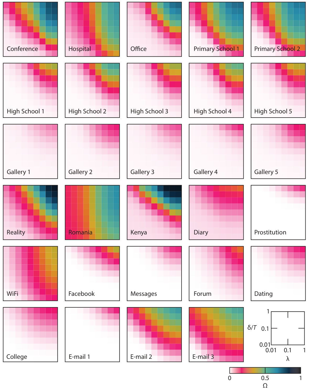 Figure 1
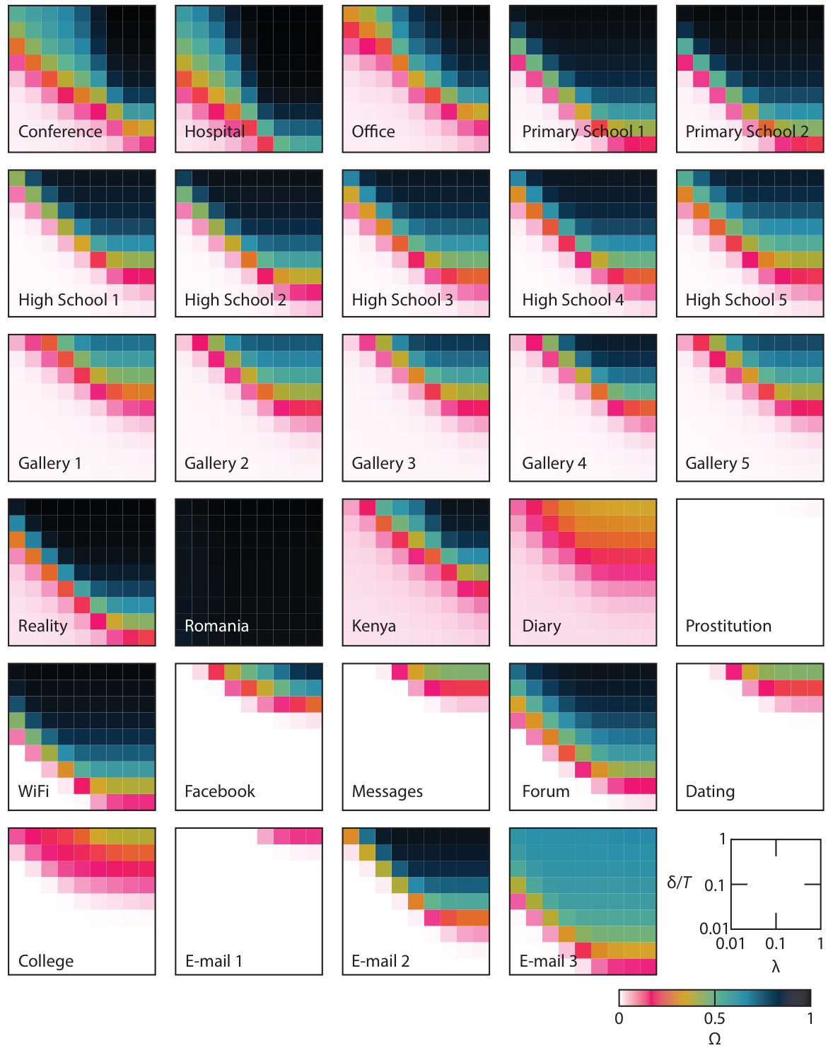 Figure 2
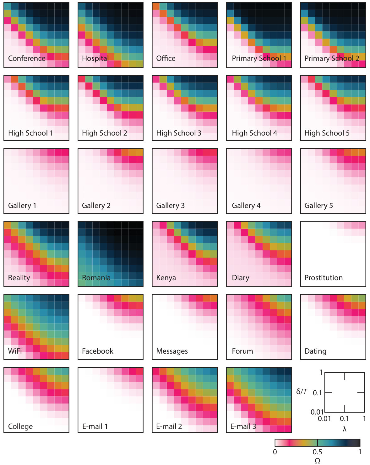 Figure 3
| Data set | Ref. | |||||
|---|---|---|---|---|---|---|
| Conference | 113 | 20,818 | 2.50d | 20s | 2,196 | conference |
| Hospital | 75 | 32,424 | 96.5h | 20s | 1,139 | hospital |
| Office | 92 | 9,827 | 11.4d | 20s | 755 | office |
| Primary School 1 | 236 | 60,623 | 8.64h | 20s | 5,901 | school |
| Primary School 2 | 238 | 65,150 | 8.58h | 20s | 5,541 | school |
| High School 1 | 312 | 28,780 | 4.99h | 20s | 2,242 | hschool |
| High School 2 | 310 | 47,338 | 8.99h | 20s | 2,573 | hschool |
| High School 3 | 303 | 40,174 | 8.99h | 20s | 2,161 | hschool |
| High School 4 | 295 | 37,279 | 8.99h | 20s | 2,162 | hschool |
| High School 5 | 299 | 34,937 | 8.99h | 20s | 2,075 | hschool |
| Gallery 1 | 200 | 5,943 | 7.80h | 20s | 714 | gallery |
| Gallery 2 | 204 | 6,709 | 8.05h | 20s | 739 | gallery |
| Gallery 3 | 186 | 5,691 | 7.39h | 20s | 615 | gallery |
| Gallery 4 | 211 | 7,409 | 8.01h | 20s | 563 | gallery |
| Gallery 5 | 215 | 7,634 | 5.61h | 20s | 967 | gallery |
| Reality | 64 | 26,260 | 8.63h | 5s | 722 | reality |
| Romania | 42 | 1,748,401 | 62.8d | 1m | 256 | roman |
| Kenya | 52 | 2,070 | 61h | 1h | 86 | kenya |
| Diary | 49 | 2,143 | 418d | 1d | 345 | read |
| Prostitution | 16,730 | 50,632 | 6.00y | 1d | 39,044 | prostitution |
| WiFi | 18,719 | 9,094,619 | 83.7d | 5m | 884,800 | wifi |
| 45,813 | 855,542 | 1,561d | 1s | 183,412 | mislove | |
| College | 1,899 | 59,835 | 193d | 1s | 13,838 | college |
| Messages | 35,624 | 489,653 | 3,018d | 1s | 94,768 | karimi |
| Forum | 7,084 | 1,429,573 | 3,141d | 1s | 138,144 | karimi |
| Dating | 29,341 | 529,890 | 512d | 1s | 115,684 | pok |
| E-mail 1 | 57,194 | 444,160 | 112d | 1s | 92,442 | ebel |
| E-mail 2 | 3,188 | 309,125 | 81d | 1s | 31,857 | eckmann |
| E-mail 3 | 986 | 332,334 | 526d | 1s | 16,064 | eml3 |
Peer Reviews
No public reviews on file for this paper yet. If you reviewed it on a platform where reviews are public (OpenReview, ICLR, NeurIPS, ICML), you can paste yours below so the community can read it here.
Videos
No videos yet. Explain this paper in a talk, walkthrough, or lecture? Add one.
Taxonomy
TopicsComplex Network Analysis Techniques · Opinion Dynamics and Social Influence · Peer-to-Peer Network Technologies
11institutetext: Institute of Innovative Research, Tokyo Institute of Technology, Tokyo, Japan, 11email: [email protected]
Probing empirical contact networks by simulation of spreading dynamics
Petter Holme
Abstract
Disease, opinions, ideas, gossip, etc. all spread on social networks. How these networks are connected (the network structure) influences the dynamics of the spreading processes. By investigating these relationships one gains understanding both of the spreading itself and the structure and function of the contact network. In this chapter, we will summarize the recent literature using simulation of spreading processes on top of empirical contact data. We will mostly focus on disease simulations on temporal proximity networks—networks recording who is close to whom, at what time—but also cover other types of networks and spreading processes. We analyze 29 empirical networks to illustrate the methods.
1 Introduction
Spreading processes111In the social science and computer science literature these are commonly known as diffusion processes. In this chapter, we stick to the natural science convention (reserving “diffusion” for processes where the total mass or amount of whatever is spreading, or diffusing, is conserved). affect people at many levels. They are the basis of innovation processes bettencourt and spreading abrahamson , they shape our opinions may15 , lifestyles christakis_fowler and they are also part of the mechanisms giving us infectious disease andersonmay ; gies ; hethcote . Even though disease spreading is a bit special and not the primary topic of this book, much of the theory of the interaction of spreading and contact structure comes from epidemiology of infectious diseases. For this reason, we will mostly use disease spreading as our model spreading dynamics and leave it to the reader to draw the analogies to other phenomena.
At the time of writing “data science” is a buzzword. One key idea behind it is that we can understand much of the social world around us by analyzing the data we create—be it from the location traces of our smart-phones phones , transportation cards sun , etc. A special type of such data records contacts between pairs of people. By contact we will mean any kind of binary interaction where something can spread from one person to the other. It could be being in physical proximity, so that disease could spread, or following someone on a social media channel, so that information could spread. A contact network could thus be thought of as a list of pairs of individuals, annotated with the time, type and locations of the interaction. In practice one usually do not have access to so much meta-information of the contacts. In many cases one must settle with only the time and identities of the individuals (a temporal network holme_saramaki ; holme_modern ; masuda_lambiotte ), or even just the identities (a static network) newman:book ; barabasi:book . On the other hand, several properties of the spreading is determined by the (temporal or static) network structure—the regularities making the network differing from a purely random one—and our understanding of how they shape the spreading dynamics is still incomplete.
One challenge for understanding how the structures of contact networks affect spreading is to be able to list and quantify the relevant structures. Structures are dependent, however, and this makes it a challenge even in the simplest case of static networks. Acquaintance networks are, for example thought to contain many triangles grano . The presence of triangles is thought to slow down spreading volz_cluster . However, this does not necessarily mean that human friendships slow down spreading. In a simple network model where the density of triangles (a.k.a. clustering coefficient) is the only structure to control, a typical network would one very densely connected core contributing with most of the triangles, not triangles distributed all over the network as empirical friendship networks have burda . Thus, there are other constraints, or structures, present in the real networks that could potentially also affect spreading phenomena. An alternative approach to controlling the density of triangles would be to take empirical networks as the starting point and simulating disease spreading directly on these. To monitor the effect of triangles one could manipulate the original network, for example by randomly rewiring links milo . Of course, one cannot isolate network structures completely—by rewiring the network, one could presumably change e.g. the average path length as well. However, one would do that from a realistic part of the space of (temporal) networks. In addition, this approach gives insights about how the network itself acts as an infrastructure for the spreading process.
The problem of straightforward approaches to understanding the effects of network structure in real spreading processes, becomes more severe the more information-rich network representation one uses. For temporal networks—where information about the time of contacts are included—this is particularly clear. It has been observed that human behavior has an intermittent, bursty behavior barabasi:burst ; goh . Subsequently, authors noticed that fat-tailed interevent time distributions—the hallmark of bursty activity—slows down spreading Karsai2011 ; vazquez . At the same time, other authors observed that simulated disease spreading was slowed down by randomizing the timing of contacts in some kinds of contact networks 50185 . There must thus be other temporal structures also controlling disease spreading. In this work, we explore methods to understand the relationship between network structure and spreading dynamics that take empirical networks, rather than network models, as starting point.
In the remainder of this chapter, we will go through some of the empirical networks authors have used, typical models of spreading processes for the purpose, randomization methods, and similar techniques. Finally, will discuss future prospects and relation to other methods.
2 Networks
In this section, we will discuss the empirical data available at the moment and some technical issues related to how to represent it mathematically or computationally.
2.1 Data sources
Proximity networks
Human proximity networks have gained much attention recently. Such data sets records when, and sometimes where, persons are in contact. At least they contain identities of the people in contact and when the contacts happen. Typically these data sets samples people connected by some circumstance—workers in the same office taro ; office , at the same hospital liljeros_giesecke_holme ; hospital ; hornbeck , students in the same school school ; hschool ; salathe ; wifi , visitors to an art gallery gallery , conference attendants conference , etc. The time limits are typically set by the experiment and in most cases running throughout one day (when the school or office is open).
Researchers have been very creative in gathering proximity networks. One common method is to equip the participants with radio-frequency identification (RFID) sensors thebook:barrat which records proximity of a couple of meters. Notably, the organization Sociopatterns (sociopatterns.org) provide many open access datasets. A similar performance to RFID sensors can be obtained by infrared taro or wireless salathe ; roman sensors. Another type of proximity measure is to use the Bluetooth channel of smart-phones. These typically records slightly more distant contacts (the order of meters). Bluetooth-based studies typically run longer and are less constrained reality ; stopczynski2014measuring ; stop .
In addition to proximity recorded by sensors, researchers have used location information to infer who is close to whom at what time. Ref. sun studies people sharing the same public transport; Ref. wifi uses a dataset of people connected to the same WiFi router. There is also a rather large field of studying patient flow within hospital systems, e.g. Refs. liljeros_giesecke_holme ; donker ; donker2012 ; walker from the records of patients and healthcare workers. A contact in such networks corresponds to two persons being at the same ward at the same time.
Yet another kind of human proximity networks (perhaps different enough to constitute a stand-alone category) is sexual networks. Classic sexual network studies do not have the time of the contacts. The only large-scale temporal network of sexual contacts we are aware of is the prostitution data of Rocha et al. prostitution where contacts with sex sellers are self-reported by the sex buyers at a web community.
Finally, although this book focuses on humans, we mention that proximity networks of animals have been studied fairly well. In particular, populations of livestock have been studied either as metapopulation networks (where one farm is one node and an animal transport between two farms is a contact), or as a temporal network of individual animals where a contact represents being at the same farm at the same time. Livestock here could refer to either cattle gates_woolhouse ; scholtes_causality ; valdano_poletto or swine konschake_components . In addition domesticated animals, researchers have also studied wild animals—zebras lahiri_berger_wolf_2007 and monkeys capuchin by GPS traces, ants thebook:charbonneau by visual observation, and birds psorakis from foraging records.
In the latter part of this chapter we will use some data set of this type as an example. In particular, we use several Sociopatterns data sets: Conference (participants of a computer science conference), Hospital (patients, doctors and nurses of a hospital), Office (workers at the same office), Primary and High School (school students), Gallery (visitors to an art gallery), and families in rural Kenya (Kenya). Some of these data sets covers several days, which we treat separately. We also use one Bluetooth data set sampled among college students in USA (Reality) and a similar dataset from Romania (Romania) sampled with WiFi technology. Finally, we use one dataset based on a diary-style survey (Diary) and one from self-reported sexual contacts with escorts (Prostitution). Statistics and references to these data sets can be found in Table 1.
Communication networks
Temporal networks of human communication are probably the largest class of systems modeled as temporal networks after proximity networks. One such type of data comes from call-data records of mobile phone operators bernhardsson ; Karsai2011 ; kovanen_motif . These use lists who called whom, or who texted whom. Typically the data sets are restricted to one operator in one country. Another type of communication networks are e-mails sampled from the accounts of a group of people during a window of time ebel ; eckmann . Yet another of this kind comes from messages at social media platforms such as Twitter romero ; sanli or Internet communities pok ; karimi_ramenzoni ; blasio ; jacobs_thefacebook ; mathiesen . A difference to proximity networks is that links in this category are naturally directed. (Later in this chapter, when we will compare networks of this kind to proximity networks and then treat contacts as undirected.)
Below we analyze one data set of wall-posts at Facebook (Facebook), one Facebook-like community for college students (College), one Internet dating service (Dating) and one film-discussion community (Forum for posts at a discussion forum, and Messages for direct, e-mail-like communication). We also study three data sets of e-mail communication E-mail 1, 2 and 3. A summary of these data sets and references can be found in Table 1.
2.2 Network representations
The basic setting we are considering is a set of nodes (sometimes called vertices). For most purposes of this chapter, the nodes represent individual people. In a static network, or graph (emphasizing the mathematical representation rather than the real system) , the nodes are connected pairwise by links (sometimes called edges) . In a temporal network the nodes are connected at specific times by contacts (sometimes called events)—triples showing that interacted with at time . An alternative way of thinking about how time enters networks is to consider nodes as a sequence of static graphs , one for every discrete time step of the data. is called the sampling time. This type of graph sequence is a special case of multilayer networks kivela_rev ; boccaletti_rev . Mathematically it is equivalent to sequences of contacts, but it does put other ideas into the mind of the user. To be specific, thinking of the system as a sequence of graphs suggests that one can first apply static network theory to each time slice individually, then aggregate these results. This could be a powerful approach in many cases, but not if the time resolution is so high that the networks are mostly very fragmented (or perhaps even empty, as the case in e.g. an e-mail network). Since paths in temporal networks need to follow the arrow of time, they are not transitive—the pairs and can have contacts without being able to influence . The reason is that all contacts between might have happen by the time the spreading has reached .
Many studies consider spreading processes in space. This is true not only for disease spreading spatial_epi , but the study of spreading of innovation (Ref. mcvoy1940patterns is an important early such reference). In principle, space can be encoded into the contacts of a network. On the other hand, in cases one are not aware of the detailed contact structure, one can resort to spatial spreading models. Spatial information can be combined with a network representation spatial and such mixed approaches are efficient in modeling multi-scale human mobility patterns (and thus contact patterns) Balcan22122009 .
3 Spreading dynamics
In this section we, discuss models of spreading phenomena that can be simulated on empirical contact sequences. It is not a complete review of the matter, but intended to give a make the latter discussion more concrete.
3.1 Epidemic spreading
The framework for modeling the spread of infections in a population is well established gies ; andersonmay . So called compartmental models divide the population into states (classes, or compartments) with respect to the disease, and prescribe transition rules between these classes. The four most common states are: susceptible (S, individuals that can get the disease, but not spread it), infectious (I, who can spread the disease), recovered (R, who can neither get or spread the disease), and exposed (E, who got the disease but can yet not infect others). The infection event typically happens between a susceptible and infectious individual. It is the only transition that requires two people to meet. Two canonical compartmental models are the SIR and SIS model. In SIR an S person can become I upon meeting an S, and an I will eventually become R. In SIS, I becomes S rather than R. There are some subtleties involved in how to implement the transitions. Mathematical epidemiology has traditionally implemented the transition from I (to R in the SIR model or S in the SIS model) as happening with a constant rate. In other words, all infected persons have the same chance of becoming uninfected every unit of time. This—constant infection rate (CIR) version—leads to an exponential distribution of the infection time, which is in contrast to observations vergu , but simplifies the calculations. An other approach—the constant infection duration (CID) version—is to model the duration of the infection as constant. As all infected nodes expose their neighbors the same amount of time, this simplifies some statistical analyses. It is also somewhat algorithmically more straightforward (but this should not be a ground for selecting the algorithm). In either of these cases, the SIR and SIS models have two parameter values. One controlling how easily a node gets infected. Another controlling how long the node stays infected. For the CIR version these are the infection and recovery rates. For the CID version they are the per-contact infection probability and disease duration .
The second ingredient in epidemic modeling is a model or data of the contact patterns. In most approaches this part comes from a simple model—the simplest being that everyone has the same chance of meeting everyone else at every time, but, in particular, with the advent of network epidemiology keeling_rev , researchers have started to study more realistic contact patterns. One approach is to construct models of human contact patterns. For example, based on the observation that sexual networks have a power-law degree distribution, researchers have studied the transmission of sexually transmitted infections on model networks with such a degree distribution lea:sex . Another approach for increased realism in disease spreading studies is to simulate the spreading on data sets of empirical contacts salathe ; 50185 ; read ; holme_tempdis ; holme_masuda_r0 . As mentioned, this approach gives more than better predictions—we can also use it to understand what structures of the contact sequence that is important, and why.
3.2 Opinion and information spreading
Much of the previous section is true for modeling of information and opinion spreading too. The main difference is that one cannot assume that such spreading is well-modeled by compartmental models. We have learned from studies of spreading in social media that individual behavior is very diverse and platform dependent. Not only do people have different activity levels, they could also follow completely different mechanisms romero ; DeMartino2015 . Sometimes authors make the distinction between simple and complex contagion weng . The former are all types of spreading phenomena where the spreading can be modeled as a probabilistic event when an S meets an I, independent of the rest of the system. Complex contagion, on the other hand can depend on more than a pairwise interaction: an opinion might need exposure from several different neighbors to spread from one vertex to another; a piece of information might spread slower with age; it could spread more easily between people that are similar to one another, etc. weng
The simplest type of complex contagion are threshold models.222An even simpler type of opinion spreading model is the voter model voter . This is a simple contagion model where random nodes copy the opinion of random neighbors. These assume that an individual adopts an idea when the exposure is over a threshold. What “exposure” means is not trivial. It could be the number of different persons that one hear an opinion from; it could also be the number of times one has heard the opinion backlund_threshold . Furthermore, for temporal networks, old exposures are not as important as more recent ones karimi ; taro_holme_threshold . Authors have modeled this by counting exposures in a time window into the past karimi_holme or assigning every contact with an exponentially decreasing importance metric taro_holme_threshold .
4 Null models, randomizations and positional comparisons
So far, we have discussed the kind of datasets available and different dynamic models of spreading phenomena. While running such simulations on the raw contact data can be interesting in its own right, it can be hard to generalize the results. As mentioned in the Introductions, one option is to compare the results to those expected from models. This approach has been a fruitful way for static networks but is challenging for more information-rich representations of the contact patterns. One reason is that it is hard to even name a reasonably complete set of simple structures in temporal networks (it is of course even harder to control them in a way such that the results are easy to interpret). An alternative approach is to draw the conclusions from comparisons. One way is to use randomize some aspect of the real data and thereby destroy some particular structure. By comparing the spreading on the original and randomized networks, one can draw conclusions about the effects of the randomized structures. By successively randomizing less and less one can, in principle, home into the important structures. One may argue that this approach is only replacing the problem of listing fundamental structures, by the problem of listing structures to randomize. However, one is certain that going from the original data to the fully randomized data, one has removed all structure there is, and thus all structure that can play a role in the spreading (even though this procedure should be coarser than ideal).
Refs. holme_saramaki ; holme_coll presents several methods of randomization. In this chapter, we will exemplify with two: Random times (RT) and Random links (RL). For RT one replaces the timestamps of contacts with random times in the interval , thus destroying several types of temporal structures including effects of: order of events, periodic changes in the overall activity, the turnover of individuals, etc. RT is thus a quite pervasive type of randomization, only conserving the number of contacts and the static network structure. One can regard RL as a topological counterpart to RT. For RT one replaces link by a link between two random nodes in the network. Thus one destroys all the topological structure, including the degree distribution.333Effectively one replaces the degree sequence by one drawn from a binomial distribution. For many applications one is rather interested in the topological structure other than the degree distribution, and would rather conserve the degree of the nodes milo , but to be able to compare the topological randomization to the temporal one, we use this definition. With the results for the original and randomized networks at hand one can see how the destroyed structure affects the spreading. This effect would typically depend on the parameter values of the spreading dynamics. To get interpretable results one typically average over many randomized data sets. The good news is that temporal networks are typically “self-averaging” in the sense that fluctuations decrease with systems size. To move further into describing how the contact structure affects the spreading one can also include measurements of (temporal or static network structure). For example, Ref. holme_masuda_r0 compares the discrepancies between two estimates of disease severity for different contact data sets. They correlate the discrepancies with measures—network descriptors—like the node and link burstiness goh , the fraction of nodes and links present throughout the sampling time, etc. From this analysis they can conclude that some types of discrepancies are more related to temporal structures, other to topological structures.
In addition to randomizing away structure, one can learn about the structure of the contact network by comparing nodes and links of within the same network. One can for example compare spreading starting at different nodes and compare the average outbreak size, time to peak prevalence or time to extinction holme_pcb ; rocha_masuda . Another approach would be to eliminate single nodes and links and study the changes of the mentioned quantities bramson .
5 Example: SIR model on empirical networks
In this section, we will present an analysis along the lines outlined above for the contact networks of Tab. 1. In Fig. 1, we show the average outbreak size (the fraction of recovered nodes at the end of the outbreak) in an SIR simulation. We use the CID version, so the two parameter values are the per-contact transmission probability and the disease duration . The infection is started by one randomly chosen node at a random time between [math] and . All data points are averaged over at least outbreak runs per networks. In Figs. 2 and 3 we show plots of as a function of and for the RT and RL randomizations, respectively. For these figures, we also average each value over randomizations.
A first thing to notice in Fig. 1 is that is increasing with both and . For some networks, reaches its maximal value , but for most it does not. For the Gallery data, Prostitution and the social media networks (Facebook, Messages, Forum, Dating, and College) there is a big overturn of agents—the individuals that are there in the beginning are not there in the end. (This is easy to imagine for the Gallery networks as a visitor to an art gallery would stay for a limited amount of time.) A low maximal can only most easily be explained by that the turnover of agents breaks many time-respecting paths so that one individual cannot infect so many others. Another explanation would be that most contacts happen in the beginning, so that by chance the network is very fragmented by the time a typical first infection event happens. Some of the networks are so dense that even for the lowest parameter values () is quite large. The most conspicuous example is perhaps Romania where both the minimum and maximum value is intermediate. At this point, it is worth noting that (unlike ) should not be understood as a parameter that is unique for one disease. It must be defined in combination with the network representation—a more restrictive definition of a contact would correspond to a larger value stop . Finally, we note that the data sets that come from the same setup (the five High School and Gallery networks looks like each other—an indication that the used methods are not sensitive occasional misinformation).
Next, we turn to the data with randomized time stamps. as a function of and is displayed in Fig. 2. The effect of the randomization is different for different data sets. For several data sets increases, at least the maximal , or sometimes throughout the parameter space. The main exception is Prostitution where the maximal decreases upon randomization. Some other data sets—the Gallery data and E-mail 1 do not change. From this we understand that given the underlying contact network, and the number of contacts between each pair of nodes, the timing of the nodes can both speed up and slow down the disease spreading. Since bursty behavior is known to slow down spreading vazquez ; Karsai2011 and the RT randomization makes contacts less bursty, we can understand that other temporal factors also determine the speed and scope of the spreading. We can also notice that the effects of RT randomization is largest for intermediate values of (of Fig. 1).
The outbreak sizes corresponding to Fig. 1 for topologically randomized datasets is shown in Fig. 3. The pattern from the RT plots of Fig. 2 remains, and is somewhat accentuated. For the RL randomized plots, reaches close to its maximum value for most of the data sets (including Gallery, where this was not true for the RT randomization). For some other datasets—Prostitution, Diary, E-mail 1 and E-mail 3—the maximal decreases going from RT to RL. In summary, most datasets we test have investigated have both temporal and topological structures that decreases the outbreak sizes. Why the opposite occasionally happens is an interesting and—at the moment of writing—not fully resolved problem. One observation is that all such data sets are fairy sparse in the sense that is small, but other structures can separate these data sets from others even more clearly. One such structure is the average duration of a link holme_liljeros . Other quantities that describe the long-term evolution of the system could also work well.
6 Discussion
In this chapter, we have pointed at some ways one can analyze empirical datasets of human interaction by simulating spreading phenomena on top of them. We have discussed data sources, network representations and some of the analysis techniques including some of the many randomization-based null-models available. The type of analysis we have outlined is not from a pipeline to handle contact data. Indeed, the analysis of temporal networks is not so developed or systematic as the ones for static networks. To understand how contact networks works, at the moment, one need to use different approaches at once (what we sketched in this chapter is one of them). Several papers that have used the same approach as this chapter do not stop after comparing the original and randomized networks, they continue to try to identify lower-level structures. For example Refs. holme_masuda_r0 ; holme_tempdis characterizes the differences between SIR spreading on the original and randomized data, then performs a regression analysis to find which low-level structural descriptor that has the highest explanatory power.
For the future, we hope it will be possible to formalize the ideas in the chapter to a more programmatic approach. In particular, it is probably possible to construct a flow-chart how to perform successive randomizations to identify the important structures for spreading on a particular data set. This would need to solve the question about how to randomize away arbitrary structures (or at least all structures that are easy to understand conceptually, thus contributing to our understanding of network dynamics). For opinion spreading problems, a major challenge is to find an appropriate microscopic model of the spreading weng .
The reference list from the paper itself. Each links out to its DOI / PubMed record.
- 1(1) L.M.A. Bettencourt, J. Lobo, D. Helbing, C. Kühnert, G.B. West, Proceedings of the National Academy of Sciences 104 (17), 7301 (2007)
- 2(2) E. Abrahamson, L. Rosenkopf, Organization Science 8 (3), 289 (1997)
- 3(3) J. Borge-Holthoefer, A. Rivero, I. García, E. Cauhé, A. Ferrer, D. Ferrer, D. Francos, D. Iñiguez, M.P. Pérez, G. Ruiz, F. Sanz, F. Serrano, C. Viñas, A. Tarancón, Y. Moreno, PLOS ONE 6 (8), 1 (2011)
- 4(4) N.A. Christakis, J.H. Fowler, New England Journal of Medicine 357 (4), 370 (2007)
- 5(5) R.M. Anderson, R.M. May, Infectious diseases in humans (Oxford University Press, Oxford, 1992)
- 6(6) J. Giesecke, Modern infectious disease epidemiology , 2nd edn. (Arnold, London, 2002)
- 7(7) H.W. Hethcote, SIAM Rev. 32 (4), 599 (2000)
- 8(8) S.E. Wiehe, A.E. Carroll, G.C. Liu, K.L. Haberkorn, S.C. Hoch, J.S. Wilson, J. Fortenberry, International Journal of Health Geographics 7 (1), 22 (2008)