On Compatible Triangulations with a Minimum Number of Steiner Points
Anna Lubiw, Debajyoti Mondal

TL;DR
This paper proves that determining whether two compatible polygons with holes can be triangulated with a limited number of Steiner points is NP-hard, highlighting computational complexity in geometric shape morphing.
Contribution
The paper establishes NP-hardness of the compatible triangulation problem with Steiner point constraints for polygons with holes, advancing understanding of geometric compatibility.
Findings
NP-hardness proven for polygons with holes
Open problem remains for simple polygons
Highlights complexity in shape morphing applications
Abstract
Two vertex-labelled polygons are \emph{compatible} if they have the same clockwise cyclic ordering of vertices. The definition extends to polygonal regions (polygons with holes) and to triangulations---for every face, the clockwise cyclic order of vertices on the boundary must be the same. It is known that every pair of compatible -vertex polygonal regions can be extended to compatible triangulations by adding Steiner points. Furthermore, Steiner points are sometimes necessary, even for a pair of polygons. Compatible triangulations provide piecewise linear homeomorphisms and are also a crucial first step in morphing planar graph drawings, aka "2D shape animation". An intriguing open question, first posed by Aronov, Seidel, and Souvaine in 1993, is to decide if two compatible polygons have compatible triangulations with at most Steiner points. In this paper…
Click any figure to enlarge with its caption.
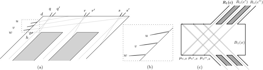 Figure 1
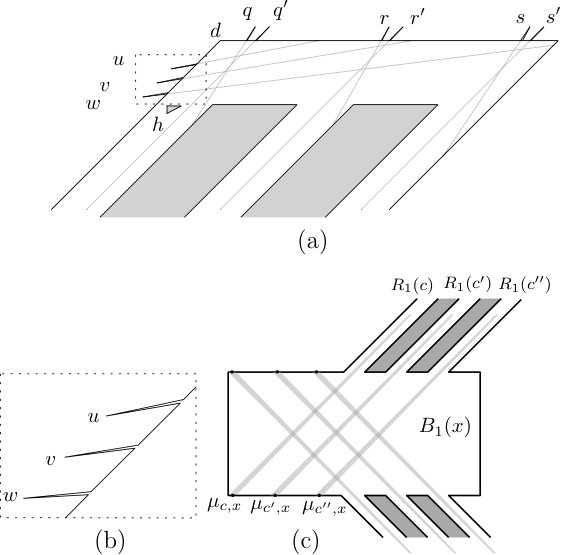 Figure 2
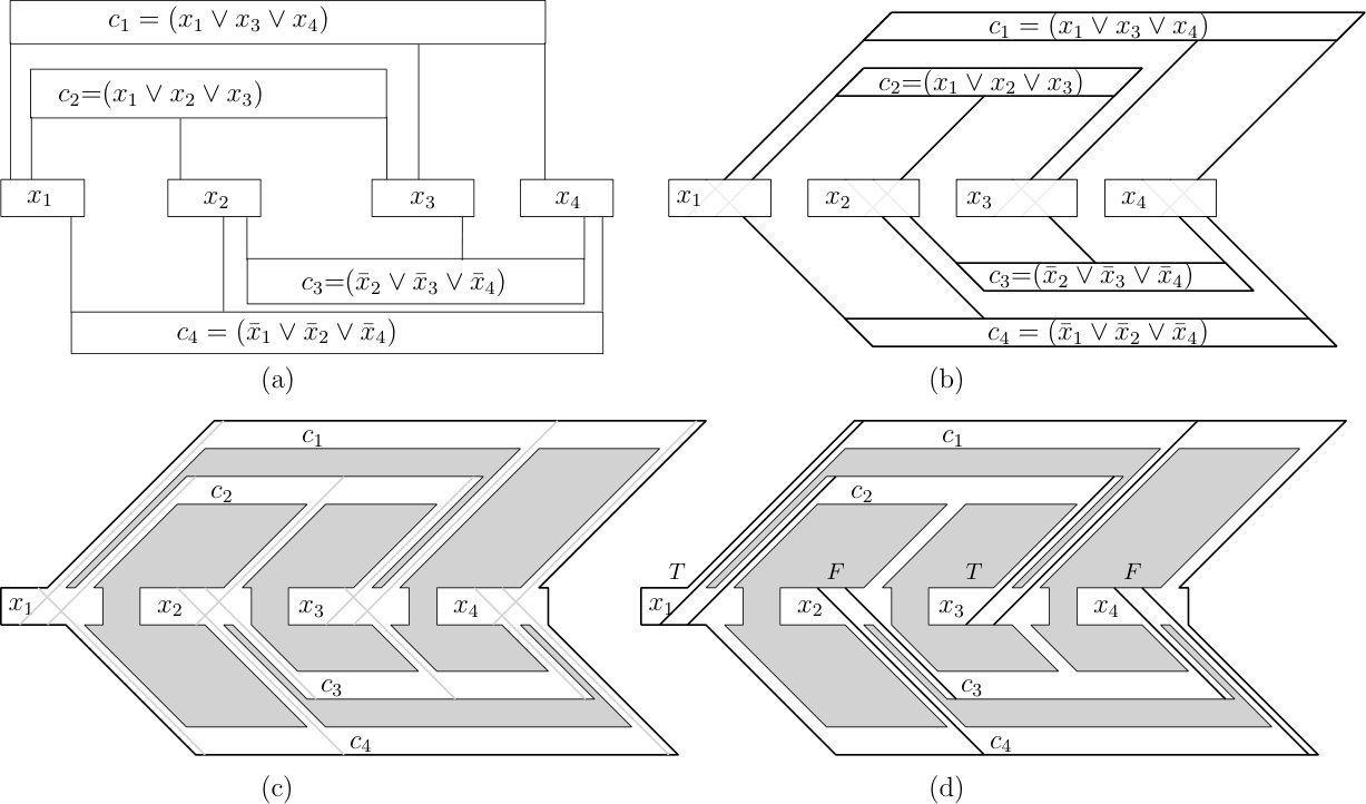 Figure 3
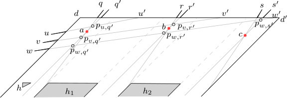 Figure 4
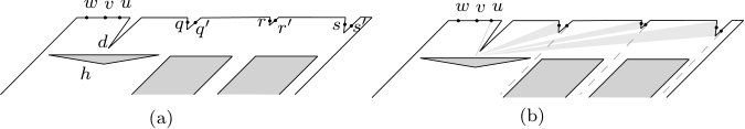 Figure 5
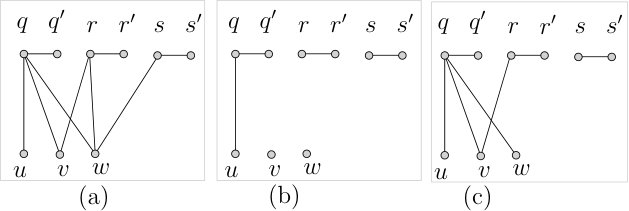 Figure 6
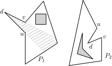 Figure 7
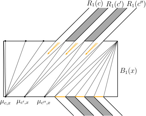 Figure 8
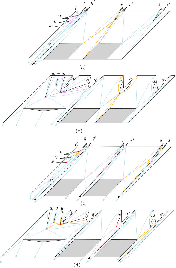 Figure 9
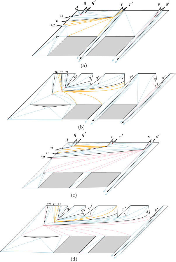 Figure 10
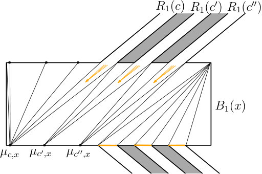 Figure 11
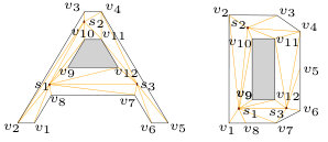 Figure 12
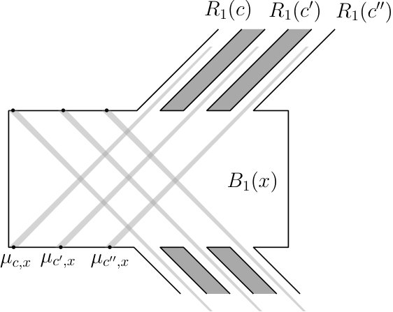 Figure 13
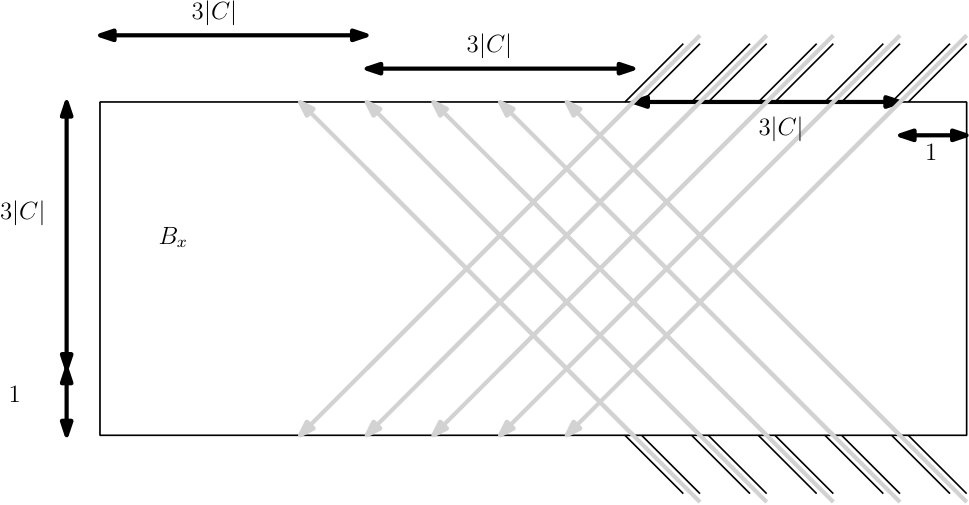 Figure 14
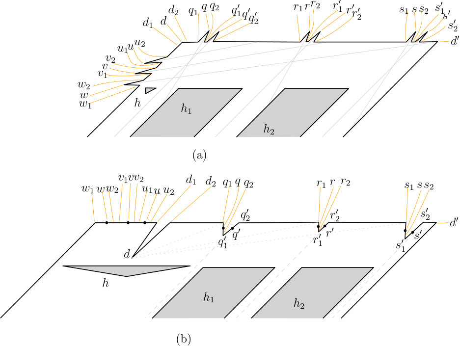 Figure 15
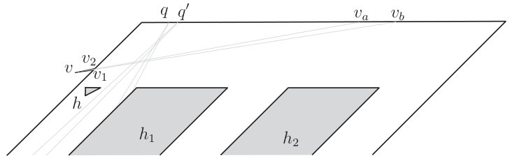 Figure 16
Peer Reviews
No public reviews on file for this paper yet. If you reviewed it on a platform where reviews are public (OpenReview, ICLR, NeurIPS, ICML), you can paste yours below so the community can read it here.
Videos
No videos yet. Explain this paper in a talk, walkthrough, or lecture? Add one.
On Compatible Triangulations with a
Minimum Number of Steiner Points††thanks: Work is supported by the Natural Sciences and Engineering Research Council of Canada (NSERC).
Anna Lubiw
Cheriton School of Computer Science, University of Waterloo, Canada {alubiw,dmondal}@uwaterloo.ca
Debajyoti Mondal
Cheriton School of Computer Science, University of Waterloo, Canada {alubiw,dmondal}@uwaterloo.ca
Abstract
Two vertex-labelled polygons are compatible if they have the same clockwise cyclic ordering of vertices. The definition extends to polygonal regions (polygons with holes) and to triangulations—for every face, the clockwise cyclic order of vertices on the boundary must be the same. It is known that every pair of compatible -vertex polygonal regions can be extended to compatible triangulations by adding Steiner points. Furthermore, Steiner points are sometimes necessary, even for a pair of polygons. Compatible triangulations provide piecewise linear homeomorphisms and are also a crucial first step in morphing planar graph drawings, aka “2D shape animation.” An intriguing open question, first posed by Aronov, Seidel, and Souvaine in 1993, is to decide if two compatible polygons have compatible triangulations with at most Steiner points. In this paper we prove the problem to be NP-hard for polygons with holes. The question remains open for simple polygons.
1 Introduction
For many computational geometry problems involving a polygon or polygonal region, the standard first step is to triangulate the region. However, for some problems, such as morphing of polygons, or finding a homeomorphism between polygons, the input consists of two polygons with a correspondence between them, and the desirable first step is to triangulate them in a consistent way. Unlike for a single polygon, it may be necessary to add new vertices, called “Steiner points.” Our paper is about this harder problem, which was called “joint triangulation” by Saalfeld [12] and “compatible triangulation” by Aronov, Seidel, and Souvaine [3].
Research on finding compatible triangulations is motivated by applications in morphing [2] and 2D shape animation [5, 15], and in computing piecewise linear homeomorphisms of polygons.
Throughout, we deal with vertex-labelled straight-line planar drawings. The most general input we consider is a polygon with holes (a polygonal region), where we allow a hole to degenerate to a single point. Two polygons are compatible if they have the same clockwise cyclic ordering of vertices. Two polygonal regions and are compatible if their outer polygons are compatible, and their holes are compatible, i.e. each hole (considered as a polygon) in corresponds to a compatible hole in . Note that the labelling provides the correspondence.
A triangulation of a polygonal region is a subdivision of its interior region into triangular faces. The vertices of are called Steiner points of . A pair of triangulations and of compatible polygonal regions and , respectively, are compatible if their faces are compatible, i.e. every face of (considered as a polygon) corresponds to a compatible face of . Again, the labelling provides the correspondence. Figure 1 illustrates a pair of compatible polygonal regions and their compatible triangulations.
Two special cases of compatible triangulations were studied independently. Saalfeld in 1987 [12] considered the case of two rectangles each with points inside them (where the correspondence between the points is given) and showed that compatible triangulations always exist. Saalfeld’s construction may require an exponential number of Steiner points [14]. Aronov et al., in 1993 [3] considered the case of simple compatible polygons. They showed that there exist compatible triangulations with Steiner points. (A similar construction was given by Thomassen in 1983 [16, Theorem 4.1].) Furthermore, Aronov et al. gave an -time algorithm to compute such compatible triangulations, and they gave examples where Steiner points are necessary. They posed as an open problem to decide if two polygons have a compatible triangulation with Steiner points, and observed that the case can be decided in polynomial time via dynamic programming.
Our Result. We show that it is NP-hard to decide if two compatible polygonal regions have compatible triangulations with at most Steiner points, where is given as part of the input.
Further Background. There are a number of further results for the case of two simple polygons. Kranakis and Urrutia [9] gave an -time algorithm to find compatible triangulations of simple compatible polygons with Steiner points, where is the number of reflex vertices. Gupta and Wenger [8] gave a polynomial-time algorithm that provides an approximation to the minimum number of Steiner points. A number of heuristic algorithms have been proposed—see e.g., [5, 15].
There is also a line of research on the case of polygons with point holes (Saalfeld’s problem). Souvaine and Wenger [14] gave an -time algorithm to compute compatible triangulations with Steiner points, and asked if there is a polynomial-time algorithm to construct compatible triangulations with the minimum number of Steiner points. Pach et al. [10] proved that Steiner points are sometimes necessary.
For the case of general polygonal regions—which encompasses both the above special cases—Babikov et al. [4] gave an -time algorithm to compute compatible triangulations with Steiner points.
One approach to computing compatible triangulations is to first compute a triangulation for one of the polygonal regions, and then draw its underlying graph into the other polygonal region using polylines for drawing edges. The edge bends give rise to the Steiner points. This idea relates to the problem of drawing a planar graph on a given set of points, where the correspondence between vertices and the points is given. Pach and Wenger [11] gave an -time algorithm to compute such an embedding with bends in total, and this was extended to deal with a bounding polygonal region in [6].
The version of the compatible triangulation problem where the correspondence between the two polygonal regions is not given is also well-studied and very relevant in practice, e.g. see [5]. In this setting, Aichholzer et al. [1] made the fascinating conjecture that for any two point sets each with points, of which lie on the convex hull, there is a mapping between them that permits compatible triangulations with no Steiner points.
2 Preliminaries
Let be a polygon, possibly with holes. Two points in are visible if the line segment between them lies strictly inside ; they are 1-bend visible if there is a point inside that is visible to both and .
A dent on the boundary of consists of three consecutive vertices of such that is convex and are reflex vertices, e.g., see the polygon in Figure 2. We refer to as the peak of the dent. The visibility region of consists of all the points inside that are visible to . An inward dent on the boundary of consists of three consecutive vertices of such that is reflex and are convex vertices. The following simple lemma about dents in compatible triangulations of polygons will be a key ingredient of our NP-hardness proof.
Lemma 1
Let and be a pair of compatible polygons. Assume that contains a dent , and let be the visibility region of in . If are not visible in , then in any compatible triangulations must be adjacent either to a Steiner point or a vertex (except and ) inside .
Proof:
Any triangulation of (even with Steiner points) must use the edge or an edge incident to . In compatible triangulations of and the edge is ruled out, and therefore must be adjacent to a Steiner point or a vertex in .
3 NP-Hardness
In this section we prove that given a pair of compatible polygonal regions , and , it is NP-hard to decide if there are compatible triangulations of and with at most Steiner points.
We reduce from the monotone rectilinear planar -SAT problem (MRP-3SAT), which is NP-complete [7]. The input of an MRP-3SAT instance is a collection of clauses over a set of Boolean variables such that each clause contains at most three literals, and is either positive (consists of only positive literals), or negative (consists of only negative literals). Moreover, the corresponding SAT-graph (the bipartite graph with vertex set and edge set appears in ) admits a planar drawing satisfying the following properties:
- - Each vertex in is drawn as an axis-aligned rectangle in .
- All the rectangles representing variables lie along a horizontal line .
- The rectangles representing positive (respectively, negative) clauses lie above (respectively, below) .
- Each edge of is drawn as a vertical line segment that connects the rectangles corresponding to and , e.g., see Figure 3(a).
The MRP-3SAT problem asks whether there is a truth assignment for satisfying all clauses in .
Given an instance of MRP-3SAT, we construct a pair of compatible polygonal regions and such that they admit compatible triangulations with at most Steiner points, if and only if is satisfiable.
Idea of the reduction:
We first ensure that every clause in has exactly three literals, by duplicating literals if necessary. Let the resulting instance be . It is straightforward to observe that is also an instance of MRP-3SAT, and is satisfiable if and only if is satisfiable. Let be the drawing corresponding to .
We modify the drawing such that the edges and vertices corresponding to the positive (resp., negative) clauses become parallelograms, slanted (resp., ) to the right, e.g., see Figure 3(b). For each clause , let denote the parallelogram corresponding to . We call the “clause region”. For each variable , let denote the rectangle corresponding to . We call the “variable region”. We call the edges of connectors and we call the connectors that are incident to the top (resp., bottom) side of top (resp., bottom) connectors of . We ensure that the extension of every top connector intersects the extensions of all the bottom connectors inside . Let the resulting drawing be . We construct and by modifying two distinct copies of .
We prove that in any compatible triangulations with Steiner points, for each clause , there is a triangulation edge that lies along one of the connectors incident to the clause region. If is positive (resp., negative) then we can set the variable corresponding to to true (resp., false) and this will satisfy the clause. We get a valid truth-value assignment because a variable region cannot contain extensions of both top and bottom connectors. Figures 3(c)–(d) illustrate a satisfying truth assignment for . On the other hand, given a satisfying truth assignment, we show how to find compatible triangulations for and using Steiner points.
3.1 Construction of Polygonal Region
We modify a copy of to construct . First we create a channel of small non-zero width around each connector so that we have a polygon with holes. We denote the copies of and in by and . We create nine dents with peaks in the boundary of , as shown in Figures 4(a)–(b). The visibility region of each dent is illustrated using gray straight lines.
As illustrated in Figure 4(a), we place a hole in the leftmost channel of , not intersecting the visibility regions of the peaks . We refer the reader to Section 4 for the formal details of the construction and the precise placement of .
We now modify the rectangles that correspond to the variables. Let be a literal and let be the corresponding rectangle in . See Figure 4(c). For every positive (resp., negative) clause containing , one or more111Recall that may contain duplicates of a literal. visibility regions corresponding to the peaks of enter . We ensure that the visibility regions entering from the top (resp., bottom) of are disjoint and only intersect the bottom (resp., top) side of . For each clause containing , we construct a vertex on the side of such that is visible to the corresponding peak of . We refer to these newly constructed points as the -points of .
3.2 Construction of Polygonal Region
We modify a copy of to construct . As in the construction of , we create a channel of small non-zero width around each connector so that we have a polygon with holes. We denote the copies of and in by and . We create four inward dents on the boundary of , and place the points , as shown in Figure 5(a). Finally, we place the hole ensuring that no peak in is 1-bend visible to , e.g., see Figure 5(b). We refer the reader to Section 4 for the formal details of the construction.
We now modify the rectangles that correspond to the literals. Let be a literal and let be the corresponding rectangle in . The modification for is analogous to that of . Specifically, for every visibility region (of some peak ) that intersects the box in , we construct a point on the boundary of box such that and are visible in . Figure 5(b) illustrates such visibilities with dashed lines.
3.3 Properties of Compatible Drawings
In this section we prove some key properties of compatible triangulations and of and , respectively. For clause , let be the clause region plus its three attached channels.
Lemma 2
If is a clause such that no peak is adjacent in to a point outside , then there are at least 6 Steiner points in .
Proof:
Consider the 9 points . In each point in this set is the peak of a dent, so by Lemma 1, each of these 9 points must be adjacent in to a vertex or a Steiner point. The only vertices visible to any of the 9 peaks are the -points visible to , but they lie outside . We assumed there is no edge from to a point outside . The other 6 peaks are not visible to any point outside . Thus each of the 9 peaks must be adjacent to a Steiner point in . No point in is visible to more than two peaks. Thus we need at least Steiner points. The only way that 5 Steiner points suffice is to use 4 Steiner points that are each adjacent to two peaks. Pairs of peaks that are visible to a common point in both and are indicated by edges in the graph shown in Figure 6(a). We require a matching of size 4 in . Observe that is bipartite so the maximum size of a matching is equal to the minimum size of a vertex cover. The set is a vertex cover of size 3. Thus there is no matching of size 4, and the Lemma follows.
Lemma 3
For any clause , there are at least 5 Steiner points in .
Proof:
Consider the triangulation of . The case where no peak has an incident edge to a point outside is covered by Lemma 2. It remains to consider the cases when there is such an edge.
Our argument will be partly about the graph (in Figure 6(a)) of pairs of peaks that are visible to a common point in both and , and partly about the geometry of . First we note that the argument used above in the proof of Lemma 2 can be strengthened to show that if we use just one edge from a peak to a point outside the clause region then we still need 5 Steiner points inside the region. In graph , observe that if one of is removed, then we have 8 vertices, and a maximum matching of size 3, which means that we can use 3 edges (Steiner points) to cover 6 vertices, leaving 2 vertices that need one Steiner point each, for a total of 5 Steiner points. It remains to consider the cases where at least two of the points have an incident edge to a point outside the clause region. We deal with the case where has such an edge and the case where has such an edge but does not.
Suppose there is an edge from to a point outside . Observe that edge cuts off the visibility regions of and . The effect on graph is to remove the edges of incident to and , e.g., see Figure 6(b). Thus we need one Steiner point for each of and , one Steiner point for (irrespective of how is connected), one Steiner point for and one more for , a total of at least 5.
Next suppose there is no edge from to a point outside of , but there is an edge from to a point outside of . The edge cuts off the visibility region of . The effect on graph is to remove the edges and , e.g., see Figure 6(c). We then need a Steiner point for (irrespective of how is connected), and for the remaining 6 vertices , we have a subgraph with a minimum vertex cover of size 2, thus a maximum matching of 2 edges (Steiner points) to cover 4 vertices, leaving 2 vertices that need one Steiner point each, for a total of 5 Steiner points.
Lemma 4
If and use Steiner points each, then for any clause , there is an edge in from at least one of to a -point.
Proof:
By Lemma 3 every region has at least 5 Steiner points. Thus every such region must have exactly 5 Steiner points and there are no Steiner points in the variable regions. Suppose there is a clause such that has no edge from or to a -point. Then there is no edge from or to a point outside . But then by Lemma 2 the clause region must have at least 6 Steiner points, a contradiction.
3.4 Reduction
Theorem 1
*The following problem is NP-hard: Given a pair of compatible polygonal regions , and , decide if and have compatible triangulations with at most Steiner points. *
Proof:
Let be an instance of MRP-3SAT, and let and be the corresponding compatible polygons, as described in Sections 3.1–3.2. Section 4 presents further details on how to construct and using a polynomial number of bits, so this is a polynomial-time reduction. We now prove that and admit a pair of compatible triangulations, each with at most Steiner points, if and only if admits a satisfying truth assignment.
We first assume that and admit compatible triangulations with at most Steiner points. By Lemma 4, for any clause there is an edge in the triangulation of from at least one peak to a -point, say . We use the edge to assign a truth value to variable . If is a positive (resp., negative) clause, then we set to true (resp., false). Clearly we have satisfied each clause. If there is a variable whose truth value is not assigned yet, then setting the truth value of arbitrarily would still keep the clauses satisfied. It remains to show that the truth-value assignment is consistent. Suppose there is a variable such that some clause forces to be true, and some other clause forces to be false. Without loss of generality we may assume that is positive and is negative. Consequently, in each of and , there exists a peak that is incident to some -point in . By construction of the -points in , the two corresponding edges cross, a contradiction.
Assume now that admits a satisfying truth assignment. We will find corresponding compatible triangulations of and . For each variable , if is set to true, then we close the channels of the negative clauses and construct the compatible triangulations of the rectangles and using the -points on the bottom side of these rectangles, e.g., see Figure 7. The construction when is set to false is symmetric.
Since every clause contains at least one true literal, for every clause , there exist one or more peaks in that are visible to their corresponding -points. We show that in each scenario, the corresponding clause gadgets can be triangulated in a compatible fashion.
Section 4 contains the remaining details of the proof of Theorem 1. These details concern the second half of the proof, where we assume that admits a satisfying truth assignment and we find corresponding compatible triangulations of and . As explained in the main text, for each variable , if is set to true, then we close the channels of the negative clauses and construct the compatible triangulations of the rectangles and using the -points on the bottom side of these rectangles, e.g., see Figure 7. The construction when is set to false is symmetric.
Since every clause contains at least one true literal, for every clause , there exist one or more peaks in that are visible to their corresponding -points. It remains to show that in each scenario, the corresponding clause gadgets can be triangulated in a compatible fashion. We only describe the case when is a positive clause. The case when is negative is symmetric.
Let be the literals of , and assume that their corresponding peaks appear in this order from left to right in .
Case 1 (): Figures 8(a)–(b) illustrate the compatible triangulations of and for the case when and . Figures 8(c)–(d) illustrate the compatible triangulations of and for the case when and . The scenarios when and , or vice versa, can be handled by switching between the local configurations corresponding to the true and false values.
Case 2 (, ): Figures 9(a)–(b) illustrate the compatible triangulations of and for the case when . The scenario when can be handled by switching between the local configurations corresponding to the true and false values.
Case 3 (, ): The compatible triangulations of and for this case are illustrated in Figures 9(c)–(d).
4 Polynomial-time Construction
In this section we describe the construction details of and . Furthermore, we show that the construction can be accomplished in polynomial time, in particular, with a polynomial number of bits for the coordinates of all points.
The construction has two stages. In the first stage we construct from (see Figures 3(a)–(b)) and in the second stage we construct and from copies of by adding the appropriate dents (see Figures 4 and 5).
For the first stage we claim that can be constructed on a polynomial-sized grid (thus, with a logarithmic number of bits per coordinate). We make each variable rectangle of width and height , as illustrated in Figure 10. The length allocated for channel attachments is to incorporate possible variable duplicates. The distance between successive -points on the bottom (top) of is at least 1. We make each clause parallelogram of height 1. The resulting drawing has height and width .
We now turn to the second stage, the construction of and . We refer the reader to Figure 13, which illustrates for each positive clause , the correspondence between the vertices of and . Observe that the left, top, and right sides of holes and have no dents added to them and remain straight line segments.
We construct the peaks of iteratively. Our plan is to first construct the visibility lines of the peaks (see Figure 11) and later enlarge these to visibility cones. Start by placing the points above the top boundary of so that the lines from them to the corresponding -points are parallel to the channel sides and centered in the channels. Next, place points to the left of and in the top half of , and choose points on the boundary of to be the endpoints of the visibility lines emanating from respectively. Specifically, choose and by taking the midpoints of the tops of and and projecting upward at .
We can explicitly compute the equations of the 6 visibility lines emanating from and we can compute the intersection points formed by them. Let be the intersection point of the visibility line of and the visibility line of , etc. We can next choose points on the visibility lines of , respectively, such that each point is in-between the appropriate points. For example, point is the midpoint of and . From these, we can construct points and their visibility lines through to appropriate points on the channels. Observe that because lie in the upper half of , points lie in the extensions of the channels, and remain to the right of , respectively.
It remains to enlarge the visibility lines to cones. We can do this by explicitly computing a tolerance such that if the width of every cone is at most inside then no visibility cone will contain points it should not, and no two visibility cones will intersect when they should not. Since we only need a lower bound on , this can be done with a polynomial number of bits. Finally, from we can explicitly choose the points where each visibility cone intersects the boundary of (see for example points and in Figure 12), and from these we can compute the dent vertices for each peak (see points and in the same figure).
Finally, we place the hole in the first channel of such that the base of is aligned with the top sides of and . Furthermore, we ensure that remains to the left of the visibility region of .
The construction of the channels and inward dents for is simpler compared to . We choose the inward dent with peak such that the entire left side of each remaining inward dent is visible to , as illustrated using dotted lines in Figure 13(b). Furthermore, we ensure that exactly one -point is visible to each of . Figure 13(b) illustrates these visibilities with dashed lines.
The placement of the triangular hole is similar to that of . Here we ensure an additional constraint that the base of must be large enough to block any -bend visibility between and .
5 Conclusion
We have proved that computing compatible triangulations with at most Steiner points is NP-hard for polygons with holes. The following questions are open:
Is the problem in NP? Is it complete for existential theory of the reals [13]? 2. 2.
What is the complexity of the problem for a pair of simple polygons? For a pair of rectangles with points inside? 3. 3.
How hard is it to decide if two polygonal regions, or two rectangles with points inside, have compatible triangulations with no Steiner points? For simple polygons, this can be decided in polynomial-time [3].
The reference list from the paper itself. Each links out to its DOI / PubMed record.
- 1[1] O. Aichholzer, F. Aurenhammer, F. Hurtado, and H. Krasser. Towards compatible triangulations. Theoretical Computer Science , 296(1):3–13, 2003.
- 2[2] S. Alamdari, P. Angelini, F. Barrera-Cruz, T. M. Chan, G. Da Lozzo, G. Di Battista, F. Frati, P. Haxell, A. Lubiw, M. Patrignani, V. Roselli, S. Singla, and B. T. Wilkinson. How to morph planar graph drawings. to appear in SIAM Journal on Computing , 2017.
- 3[3] B. Aronov, R. Seidel, and D. L. Souvaine. On compatible triangulations of simple polygons. Comput. Geom. , 3:27–35, 1993.
- 4[4] M. Babikov, D. L. Souvaine, and R. Wenger. Constructing piecewise linear homeomorphisms of polygons with holes. In Proceedings of the 9th Canadian Conference on Computational Geometry, Kingston, Ontario, Canada , 1997.
- 5[5] W. V. Baxter III, P. Barla, and K.-i. Anjyo. Compatible embedding for 2D shape animation. IEEE Transactions on Visualization and Computer Graphics , 15(5):867–879, 2009.
- 6[6] T. M. Chan, F. Frati, C. Gutwenger, A. Lubiw, P. Mutzel, and M. Schaefer. Drawing partially embedded and simultaneously planar graphs. Journal of Graph Algorithms and Applications , 19(2):681–706, 2015.
- 7[7] M. de Berg and A. Khosravi. Optimal binary space partitions in the plane. In Proceedings International Computing and Combinatorics Conference (COCOON 2010) , volume 6196 of LNCS , pages 216–225. Springer, 2010.
- 8[8] H. Gupta and R. Wenger. Constructing pairwise disjoint paths with few links. ACM Transactions on Algorithms , 3(3):26, 2007.