Dissecting Multi-Photon Resonances at the Large Hadron Collider
B.C. Allanach (1), D. Bhatia (2), A.M. Iyer (2) ((1) Cambridge (2), TIFR)

TL;DR
This paper explores how multi-photon resonances at the LHC can mimic two-photon signals due to collinear decay photons, proposing photon jet substructure analysis to distinguish scenarios and infer particle properties.
Contribution
It introduces a method using photon jet substructure variables to differentiate multi-photon decay scenarios from direct two-photon decays at the LHC.
Findings
Photon jet substructure helps distinguish multi-photon from two-photon signals.
Pseudorapidity gap distributions reveal spin information of particles.
Photon jet mass analysis provides insights into the mass of intermediate particles.
Abstract
We examine the phenomenology of the production, at the 13 TeV Large Hadron Collider (LHC), of a heavy resonance , which decays via other new on-shell particles into multi- (i.e.\ three or more) photon final states. In the limit that has a much smaller mass than , the multi-photon final state may dominantly appear as a two photon final state because the s from the decay are highly collinear and remain unresolved. We discuss how to discriminate this scenario from : rather than discarding non-isolated photons, it is better instead to relax the isolation criterion and instead form photon jet substructure variables. The spins of and leave their imprint upon the distribution of pseudorapidity gap between the apparent two photon states. Depending on the total integrated luminosity, this can be used in many cases to…
Click any figure to enlarge with its caption.
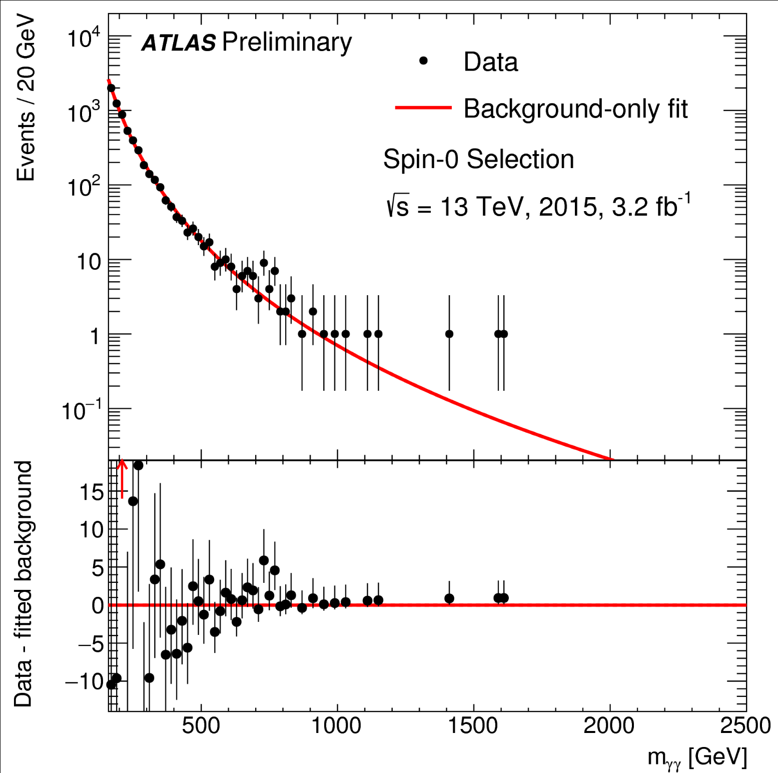 Figure 1
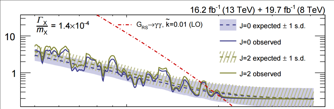 Figure 2
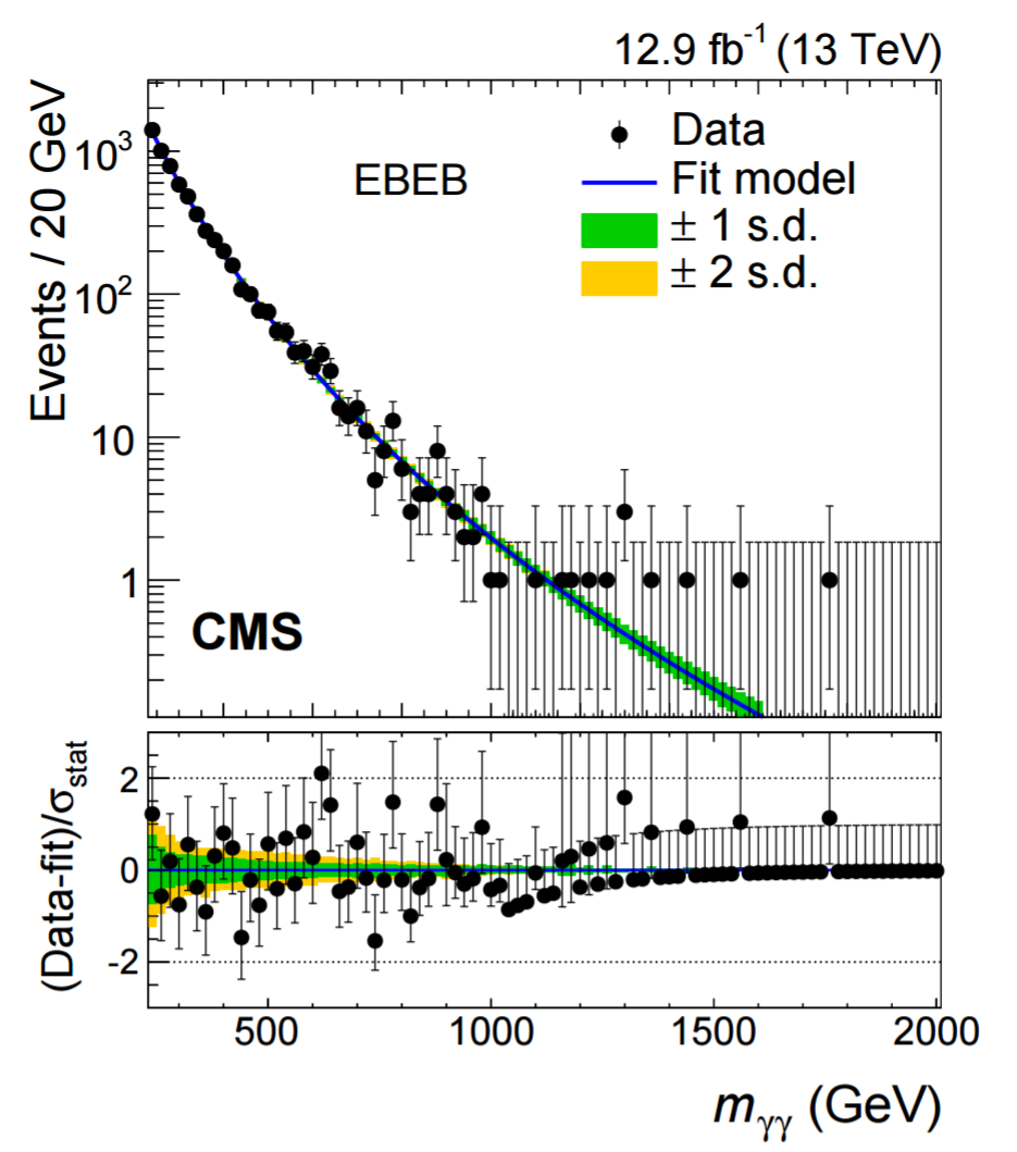 Figure 3
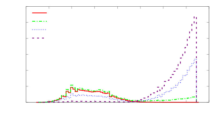 Figure 4
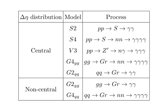 Figure 5
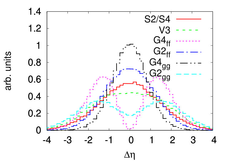 Figure 6
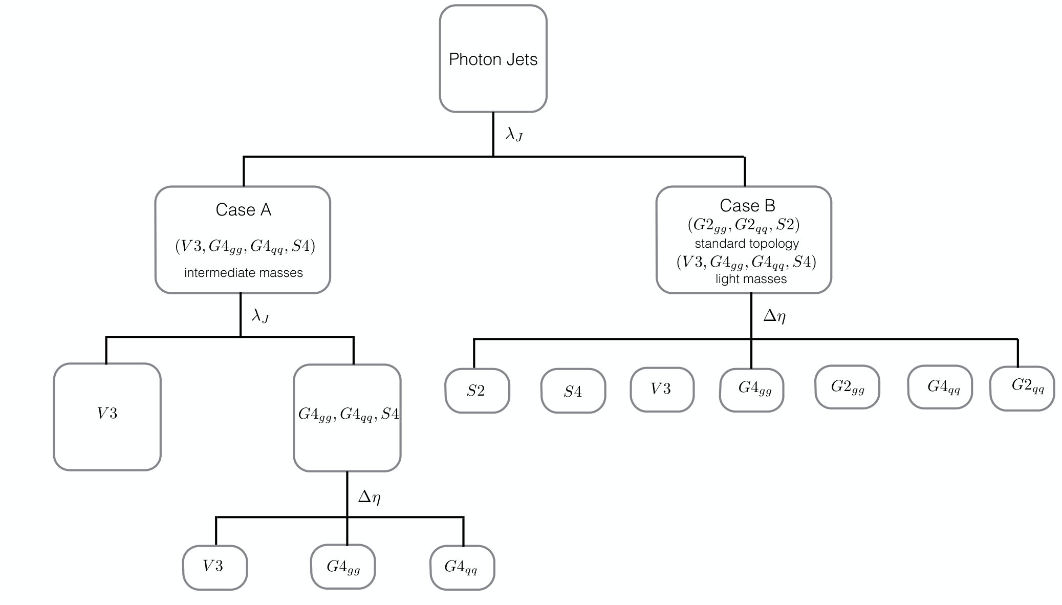 Figure 7
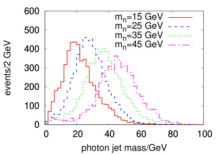 Figure 8
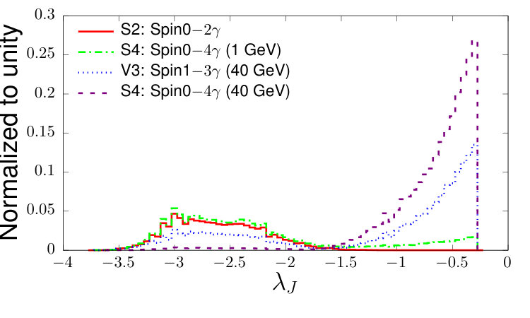 Figure 9
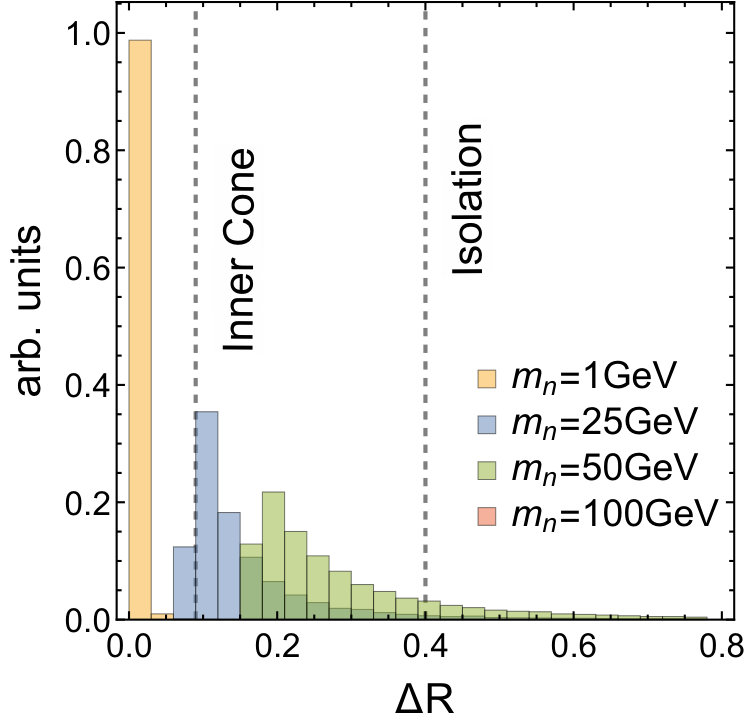 Figure 10
 Figure 11
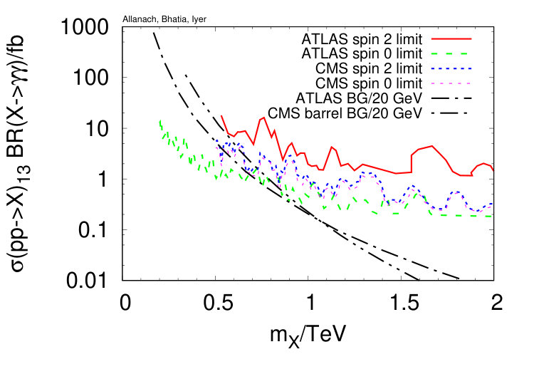 Figure 12
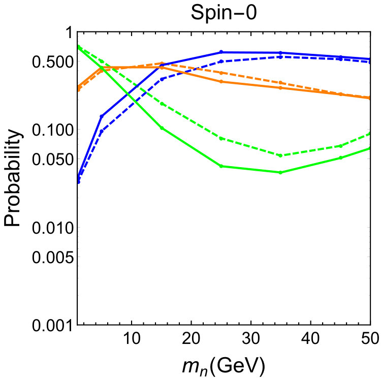 Figure 13
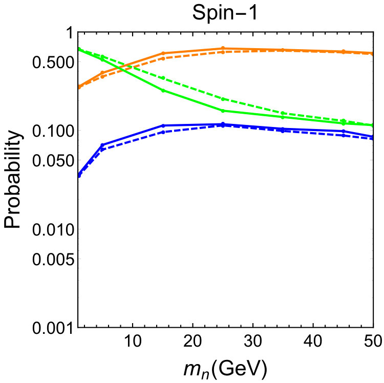 Figure 14
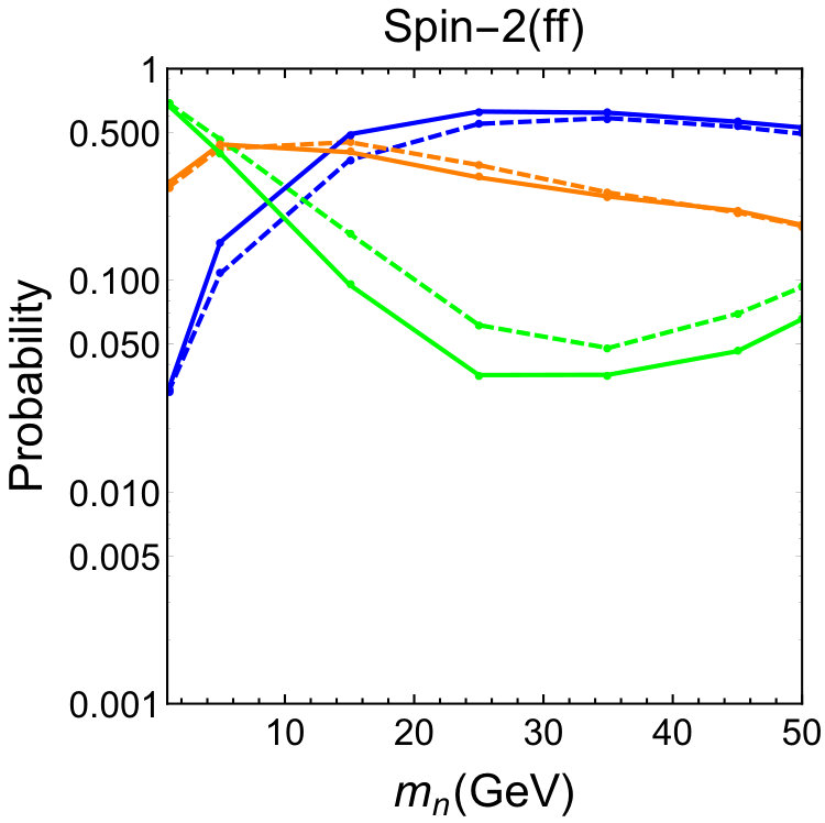 Figure 15
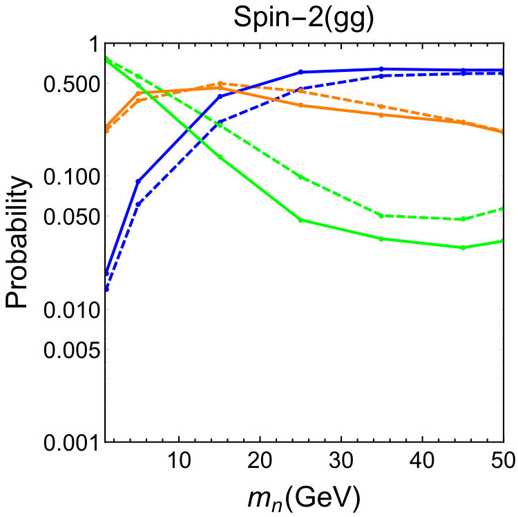 Figure 16
| Spin of | Spin of | Number of photons |
| 0 | 0 | + |
| 2 | + | |
| 1 | 0 | + |
| 2 | + | |
| 2 | 0 | + |
| 2 | + |
| Model | Process |
|---|---|
| Model | |||||||
|---|---|---|---|---|---|---|---|
| Central | Non central | ||||||
| 22 | 13 | ||
| 29 | 4 | ||
| 19 | 5 |
| 272 | 27 | 15 | 91 | 14 | |||
| 255 | 26 | 15 | 96 | 13 | |||
| 260 | 248 | 54 | 9 | 37 | 21 | ||
| 32 | 31 | 65 | 5 | 13 | 38 | ||
| 23 | 24 | 14 | 6 | 54 | 4 | ||
| 102 | 110 | 44 | 12 | 40 | 8 | ||
| 19 | 18 | 28 | 37 | 5 | 12 |
Peer Reviews
No public reviews on file for this paper yet. If you reviewed it on a platform where reviews are public (OpenReview, ICLR, NeurIPS, ICML), you can paste yours below so the community can read it here.
Videos
No videos yet. Explain this paper in a talk, walkthrough, or lecture? Add one.
Dissecting Multi-Photon Resonances at the Large Hadron Collider
B.C. Allanach
Department of Applied Mathematics and Theoretical Physics, Centre for Mathematical Sciences,
University of Cambridge, Wilberforce Road, Cambridge, CB3 0WA, United Kingdom
D. Bhatia
Department of Theoretical Physics, Tata Institute of Fundamental Research, Homi Bhabha Road, Colaba, Mumbai 400 005, India
Abhishek M. Iyer
Department of Theoretical Physics, Tata Institute of Fundamental Research, Homi Bhabha Road, Colaba, Mumbai 400 005, India
Abstract
We examine the phenomenology of the production, at the 13 TeV Large Hadron Collider (LHC), of a heavy resonance , which decays via other new on-shell particles into multi- (i.e. three or more) photon final states. In the limit that has a much smaller mass than , the multi-photon final state may dominantly appear as a two photon final state because the s from the decay are highly collinear and remain unresolved. We discuss how to discriminate this scenario from : rather than discarding non-isolated photons, it is better instead to relax the isolation criterion and instead form photon jet substructure variables. The spins of and leave their imprint upon the distribution of pseudorapidity gap between the apparent two photon states. Depending on the total integrated luminosity, this can be used in many cases to claim discrimination between the possible spin choices of and , although the case where and are both scalar particles cannot be discriminated from the direct decay in this manner. Information on the mass of can be gained by considering the mass of each photon jet.
††preprint: DAMTP-2017-28, TIFR/TH/17-29
I Introduction
The Standard Model (SM) of particle physics has been extensively tested to a great degree of accuracy. The discovery of a particle whose properties are so far consistent with those predicted for the SM Higgs boson have further fuelled the searches for Beyond the Standard Model (BSM) physics. The typical signatures employed in the search for these new physics scenarios involve different combinations of hard isolated photons, hard jets, hard isolated leptons and large missing transverse momentum. The presence of isolated leptons and isolated photons in a given final state is useful in significantly depleting SM backgrounds. The discovery of the Higgs boson in the di-photon channel Aad et al. (2012); Chatrchyan et al. (2012) has lead to an increased interest in the final state. A hunt for a putative heavy resonance enjoys enhanced sensitivity because SM backgrounds reduce quickly at larger di-photon invariant masses . Fits to the distribution are obtained by both the ATLAS and CMS by assuming simple functional forms. The central values of the fitted forms for 13 TeV LHC collisions are shown in Fig. 1. Such cross-sections depend upon the cuts and details of the analysis in question, and we have plotted the central value of the cross-section within bins of 20 GeV width obtained from the fit. The CMS analysis Khachatryan et al. (2016) displayed uncertainties, which are nonetheless small (even to the right-hand side of the curve they are small). Fig. 1 also shows the 95 confidence level upper limits on the production cross-section of a narrow resonance (we call this resonance ) that decays into a two-photon state from ATLAS and CMS. The resonant di-photon channel is then assumed to be
[TABLE]
where is electrically neutral and can either be a spin [math] or spin resonance, whereas is the remnant of the proton (for example, formed by spectator quarks), which tends to remain close to the beam-line and hence undetected. Below, we shall ignore , since it is not relevant to the phenomenology that we discuss. There are quantitative differences if one takes the assumption of a broad resonance, but the picture is still roughly the same: for resonances of a mass larger than 1 TeV, the cross section times branching ratio upper limit from current experimental searches lies somewhere between 0.1 fb and 1 fb. It is clear from the figure that other assumptions about the resonance , such as its spin, also affect the numerical value of the bound (this is because the acceptance of the signal changes). Assumptions about its production process: in particular, whether it is produced by quarks or gluons111For example, the spin 2 Randall-Sundrum graviton Randall and Sundrum (1999) has a well defined ratio of production cross-sections between and , depending upon its mass Allanach et al. (2000)., also affect the signal acceptance and hence the bound.
Heavy scalars are can result from models which contain two higgs doublets Djouadi (2008), supersymmetric extensions of little Higgs models Roy and Schmaltz (2006); Csaki et al. (2009) or extra-dimensional frameworks with bulk scalars Gherghetta and Pomarol (2000). Heavy gravitons can be attributed to the Kaluza Klein excitations of higher-dimensional gravity arising in either warped Randall and Sundrum (1999) or flat Appelquist et al. (2001) geometries. The possibility of a spin 1 particle directly decaying to di-photons is forbidden by the Landau-Yang theorem Landau (1948); Yang (1950)
In some models, the heavy resonance may decay into or , where is an additional light particle, may further decay into photons leading to a multi-photon222In the present paper, whenever we refer to multi-photon final states, we refer to three or more photons. final state. Examples of such models include hidden valley models Strassler and Zurek (2007, 2008), the next-to-minimal supersymmetric standard model (NMSSM) Ellwanger et al. (2010) or Higgs portal scenarios Schabinger and Wells (2005). There was an 8 TeV ATLAS search for a heavy resonance decaying into three and four photon states in Ref. Aad et al. (2016). For a mass of greater than 10 GeV, and a scalar of mass 600 GeV, the upper bound on cross section times branching ratios was 1 fb. For a particle of mass 100-1000 GeV, the bound on cross-section times branching ratio into a three-photon final state (and mass in the range 40-100 GeV) was found to be between 35-320 fb. However, in the limit where , photons from will be highly collimated, thereby creating the illusion of a di-photon final state from the detector point of view. Describing angles in terms of the pseudorapidity and the asimuthal angle around the beam , the angular separation between two photons may be quantified by . Neglecting its mass, the opening angle between the two photons coming from a highly boosted on-shell is
[TABLE]
purely from kinematics (this was calculated already in the context of boosted Higgs to decays Butterworth et al. (2008)), where and are the momentum fractions of the photons333The decay is strongly peaked towards the minimum opening angle Chala et al. (2016).. Thus,
[TABLE]
In the limit , and the two photons from are collinear, appearing as one photon; thus several possible interpretations can be ascribed to an apparent di-photon signal.
Below, we shall examine the phenomenology of apparent resonances, ignoring backgrounds. For this to be a good approximation, we require that the background is small compared to the signal cross-section. Fig. 1 shows that for GeV, there is parameter space where this is the case, i.e. where is well above the background but below the current experimental limits. The scenarios corresponding to different spins of and may be characterised by distributions of between the apparent di-photon states. Differences in the predicted distributions allows us to estimate the minimum number of events needed to discriminate between the different cases. In the event that the mass of the intermediate state is not too small, such that the photons from it can often be resolved, the multi-photon topology can be distinguished from the di-photon topology using the substructure of photon jets Ellis et al. (2013a, b). However, in the limit , it is hard to resolve the photons from .
There has been earlier work on heavy spin discrimination in a truly di-photon final state: telling spin 0 from spin 2 Kumar et al. (2011); Alves (2012); Pankov and Tsytrinov (2012). However, our paper goes beyond these: we consider multi-photon cases which only appear to be di-photon cases at the first glance.
It will be useful for us to categorise models’ signatures into 2 classes: the first is multi-photon signals, where is large enough for the photons (from ) to be detected by different cells of the electromagnetic calorimeter, but small enough so that they produce the illusion of a single photon. The other category includes both the standard di-photon topology and the multi-photon topology in the limit . Each apparent photon lies within a single cell of the electromagnetic calorimeter. These cases might be discriminated by photon jet substructure properties. We shall use substructure variables to identify the fundamental nature of the topology and conventional kinematic variables to distinguish the different spin possibilities in each case.
The paper is organised as follows: in section II we set up extensions to the SM Lagrangian which can predict heavy di-photon or multi-photon resonances. The finite photon resolution of the detector is discussed in section III. In Section IV, isolation criteria are removed and photon-jets are adopted. Substructure and kinematic observables are then used to distinguish the different scenarios. In section V we introduce the statistics which tell us how many measured signal events will be required to discriminate one set of spins from another, whereas we cover how one can constrain the mass of the intermediate particle in section VI. We conclude in section VII. Appendix A contains some details about model parameters.
II Model description
In this section we describe the minimal addition to the SM Lagrangian which can give rise to heavy resonant final states made of photons. We make no claims of generality: various couplings not relevant for our final state or production will be neglected. However, we shall insist on SM gauge invariance. Beginning with the di-photon final state, a minimal extension involves the introduction of a SM singlet heavy resonance . We assume that any couplings of new particles such as the (and the , to be introduced later) to Higgs fields or bosons are negligible. Eq. 4 gives an effective field theoretic interaction Lagrangian for the coupling of to a pair of photons, when is a scalar (first line) or a graviton (second line).
[TABLE]
where is the stress-energy tensor for the field and the are effective couplings of mass dimension -1. is the field strength tensor of the photon (this may be obtained in a SM invariant way from a coupling involving the field strength tensor of the hypercharge gauge boson), whereas is the field strength tensor of a gluon of adjoint colour index . As noted earlier, the direct decay of a vector boson into two photons is forbidden by the Landau-Yang theorem Landau (1948); Yang (1950). Since is assumed to be a SM singlet, there are no couplings to SM fermions, which are in non-trivial chiral representations when it is a scalar.
The presence of an additional light scalar SM singlet in the theory (), with masses such that , opens up another decay mode: . Lagrangian terms for these interactions are
[TABLE]
where has mass dimension 1. may further decay into a pair of photons leading to a multi-photon final state through a Lagrangian term
[TABLE]
Although we assume that is electrically neutral, it may decay to two photons through a loop-level process (as is the case for the Standard Model Higgs boson, for instance). Alternatively, if is a spin 1 particle, it could be produced by quarks in the proton and then decay into . The Lagrangian terms would be
[TABLE]
where are dimensionless couplings, is a right-handed quark, is a left-handed quark doublet and . The decay would have to be a loop-level process, as explicitly exemplified in Ref. Chala et al. (2016), since electromagnetic gauge invariance forbids it at tree level. A spin 1 particle may not decay into two identical spin 0 bosons due to Bose symmetry: the daughters must be symmetric under interchange, meaning they must have even orbital angular momentum . Then it is impossible to conserve total angular momentum since the initial state has and the final state has even.
For scalar then, we have a potential four photon final state if is spin 0 or spin 2 and a potential three photon final state if is spin 1 as shown in Eq. 8:
[TABLE]
If the mass of the intermediate scalar is such that , its decay products are highly collimated because the is highly boosted. It thereby results in a photon pair resembling a single photon final state. This opens up a range of possibilities with regards to the interpretation of the apparent di-photon channel. Above, we have assumed the intermediate particle to be a scalar while considering different possibilities for the spin of . Table 1 gives possible spin combinations for the heavy resonance and the intermediate particle leading to a final state made of photons. The third column gives the number of photons for each topology, grouped in terms of collimated photons that may experimentally resemble a single photon in the limit. The spin 1 example was already proposed as a possible explanation Chala et al. (2016) for a putative 750 GeV apparent di-photon excess measured by the LHC experiments (this subsequently turned out to be a statistical fluctuation).
In this work, we shall focus on the case where is a scalar. However, the techniques developed in this paper can be extended to cases where is spin 2 as well (but not spin 1, since would then be forbidden by the Landau-Yang theorem). In the next section we will describe the scenario under which the process in Eq. 8 can mimic a truly di-photon signal.
III The size of a photon
In a collider environment, any given process can be characterised by a given combination of final states. These final states correspond to different combinations of photons, leptons (electrons and muons), jets and missing energy. They can be distinguished by the energy deposited by them in different sections of the detector. In a typical high energy QCD jet, most of the final state particles (roughly 2/3) are charged pions whereas neutral pions make up much of the remaining 1/3 Ellis et al. (2013a). The constituents of a jet primarily deposit their energy in the hadronic calorimeter (HCAL) while the decay of a neutral pion ensures that it shows up in the electromagnetic calorimeter (ECAL). Thus most of the constituents of the jet pass through the ECAL and deposit their energy in the HCAL. Photons and electrons deposit their energy in the ECAL, on the other hand. They can be distinguished by mapping the energy deposition to the tracker (which precedes the calorimeters). Apart from the tracker, electrons and photons are similar in appearance, from a detector point of view. Muons are detected by the muon spectrometer on the outside of the experiment.
We shall now go on to discuss the relevant parts of the detectors and experimental analyses. The actual construction and workings of the detector are of course much more detailed than we, outside of the experimental collaborations, have tools for dealing with. We therefore characterise the cuts and detector response in in broad brush strokes. With this in mind, the experimental sensitivity to detect a single photon is subject to the following two criteria:
(a) Dimensions of the ECAL cells: The ATLAS and CMS detectors have slightly different dimensions for the ECAL cells. ATLAS has a slightly coarser granularity with a crystal size of in . In comparison, CMS has a granularity of in . CMS and ATLAS have a layer in their electromagnetic calorimeters with finer segmentation (in ATLAS, this is called ‘layer 1’) but worse segmentation, which could also be employed in analyses looking for resonances into multi-photon final states. The level of ECAL modelling including this layer is beyond the scope of this paper, and so we do not discuss it further. However, we bear in mind that information from the layer 1 may be used in addition to the techniques developed in this paper. Any estimates of sensitivity (which come later) are therefore conservative in the sense that additional information from layer 1 could improve the sensitivity. High energy photons will tend to shower in the ECAL: this is taken into account by clustering the cells into cones of size . Thus if two high energy signal photons are separated a distance , they are typically not considered to be resolved by the ECAL since it could be a single photon that is simply showering.
(b) Photon isolation: In ATLAS and in CMS, a photon is considered to be isolated if the magnitude of the vector sum of the transverse momenta () of all objects with is less than 10 of its . Qualitatively, this corresponds to the requirement that most of the energy is carried by the photon around which the cone is constructed. This criterion is required in order to distinguish a hard photon from a photon from a decay.
However, it is possible that certain signal topologies may give rise final state photons that are separated by a distance . For instance, consider the process given in Eq. 8. The particle can either be a scalar or a graviton. For concreteness, let us assume that is a scalar. In this case, a four photon final state resulting from would appear to be a di-photon final state. However, as increases, eventually and the number of resolved final state photons will increase. Similar arguments hold for the case where particle is a spin 1 state. For a given mass of , the eventual number of detected, isolated and resolved photons depends on the granularity of the detector and is expected to be slightly different for both the CMS and ATLAS.
To approximate the acceptance and efficiency of the detectors for our signal process, we perform a Monte-Carlo simulation using the following steps:
- •
The matrix element for our signal process is generated in MadGraph5 aMC@NLO Alwall et al. (2014) by generating the Feynman rules for the process with FEYNRULES Christensen and Duhr (2009). We set as specified in Appendix A, and in the model file. MadGraph5 then calculates the width of the : GeV depending on the model, so the heavy resonance is narrow444The light resonance is also narrow, since .. Events are generated at 13 TeV centre of mass energy using the NNLO1 Ball et al. (2013) parton distribution functions.
- •
For showering and hadronisation, we use PYTHIA 8.2.1 Sjostrand et al. (2008). The set of final state particles is then passed through the DELPHES 3.3.2 detector simulator de Favereau et al. (2014).
We use the DELPHES 3.3.2 isolation module for photons and we impose a minimum requirement of GeV on each isolated photon.
Figure 2 shows the probabilities of detecting the different number of detected, resolved, isolated photons in the final state for a produced for ATLAS (dashed) and CMS (solid). If GeV or , DELPHES records a zero efficiency for the photon, and it is added to the ‘0 photon’ line. In the rest of the detector, DELPHES assigns between a 85 and a 95 weight for the photon (the difference from 100 is also added to the ‘0 photon’ line in the figure). A few of the simulated photons from the additionally fail the GeV cut: these are not counted in the figure, and so the curves do not add exactly to 1.
The probabilities are shown for different possibilities of the spin of , as shown by the header in each case. The bottom row corresponds to spin 2 when it is produced by fusion (left) and annihilation (right). Spin 1 corresponds to , whereas the other cases all correspond to a decay chain. The effective number of detected photons can be reduced by them not appearing in the fiducial volume of the detector (i.e. ), or by them not being isolated (in which case both photons are rejected) or resolved (in which they count as one photon). We note that for each spin case, in the low limit, the is most likely to be seen as two resolved, isolated photons because each photon pair is highly collimated.
We note first that the probability for detecting 0, 1 or 2 resolved, isolated photons for the spin 2 case does not depend much on whether it is produced by a hard collision or a hard collision. An interesting trend is observed for the spin 0 and spin 2 cases, where the two photon probability has a minimum at GeV. At GeV, the photon pair from an are often separated by and fail the isolation criterion because the two photons have similar . Fig. 3 gives the distribution of between the photon pair coming from as a function of its mass, and illustrates the preceding point. For light masses ( GeV) it is clear that both signal photons are within . For intermediate masses GeV, most photons are within , whereas for GeV, a good fraction are already isolated photons, having . Using an estimate from Eq. 3, we deduce that events with four isolated signal photons are expected to be evident only in the m_{n}\raise 1.29167pt\hbox{;>\kern-7.5pt\raise-4.73611pt\hbox{\sim;}}120 GeV region for GeV.
The spin 1 case in comparison, has a significantly lower zero photon rate for GeV, as the process is characterised by a single photon and two collimated photons. Thus, unless the single photon is lost in the barrel or lost because of tagging efficiency, it will be recorded even if the collimated photons fail the isolation criterion.
IV Photon Jets
Since we wish to describe collimated and non-isolated photons in more detail (since, as the previous section shows, these are the main mechanisms by which signal photons are lost), we follow refs. Ellis et al. (2013b, a) and define photon-jets. For this, we relax the isolation criteria and work with the detector objects, i.e. the calorimetric and track four vectors. The calorimetric four vectors for each event are required to satisfy the following acceptance criteria:
[TABLE]
while only tracks with GeV are accepted. These calorimetric and track four vectors are clustered using FASTJET 3.1.3 Cacciari et al. (2012) using the anti- Cacciari et al. (2008) clustering algorithm with . The tracks’ four vectors are scaled by a small number and are called ‘ghost tracks’: their directions are well defined, but this effectively scales down their energies to negligible levels to avoid over counting them (the energies are then defined from the calorimetric deposits). The photon jet size is chosen to coincide with the isolation separation of the photon described in Section III. The anti- clustering algorithm ensures that the jets are well defined cones (similar to the isolation cone) and clustered around a hard momentum four vector, which lies at the centre of the cone. Thus for our signal events, the jets are constructed around the photon(s). These typically have a large , since they are produced from a massive resonance.
Since these jets are constructed out of the calorimetric (and ghost track) four vectors, they constitute a starting point for our analysis. At this stage, while a QCD-jet (typically initiated by a quark or gluon) is on the same footing as a photon jet, they can be discriminated from each other555Here we have not implemented such cuts, since we only simulated signal. by analysing different observables:
- •
Invariant mass cut: We would demand the invariant mass of the two leading photon jets to be close to the mass of the observed resonance, reducing continuum backgrounds.
- •
Tracks: QCD jets are composed of a large number of charged mesons which display tracks in the tracker before their energy is deposited in the calorimeter666A gluon initiated jet typically has a larger track multiplicity than a quark initiated jet. Bhattacherjee et al. (2015). The track distribution for a QCD jet typically peaks at higher values of the number of tracks compared to a photon jet which peaks at zero tracks.
- •
Logarithmic hadronic energy fraction (): This variable is a measure of the hadronic energy fraction of the jet. For a photon jet most of the energy is carried by the hard photon(s). As a result, this jet will deposit almost all of its energy into the ECAL, which is in stark contrast with a QCD jet. This can be quantified by constructing the following substructure observable Ellis et al. (2013b, a):
[TABLE]
where is the total energy in the jet deposited in the HCAL plus that deposited in the ECAL, whereas is the energy of each jet sub-object that is deposited in the HCAL. is large and negative for a photon jet, while it peaks close to for a QCD jet, since charged pions constitute around of the jet constituents. We would require the leading jet to have , corresponding to very low hadronic activity.
Under these cuts, the fake rate should reduce to less than Ellis et al. (2013b, a). Removing photon isolation and instead describing the event in terms of photon jets is advantageous because it helps discriminate the standard di-photon decay in Eq. 1 from the decay to more than two photons in Eq. 8. However, it still fails in the limit , as we shall see later. Taking photon jets as a starting point, we shall devise strategies where we may discern the nature of the topology and glean information about the spins of the particles involved.
IV.1 Nature of the topology
In this section we identify variables that aid in identifying the topology of the signal process and the spin of . We begin by listing different cases we would like to discriminate between in Table 2. In the event of an observed excess in an apparent di-photon final state, we would relax the isolation criteria and define photon jets. Analysing the photon jets’ substructure will help measure the number of hard photons within each jet. The difference in substructure for a photon jet with a single hard photon as opposed to several hard photons can be quantified by Ellis et al. (2013b, a):
[TABLE]
This can be understood as follows:
- •
Hard photon jets are re-clustered into sub-jets.
- •
denotes the of the leading sub-jet (i.e. the sub-jet with the largest ) within the jet in question, whilst is the of the parent jet.
- •
For a ‘single pronged’ photon jet, . Thus is negative, with a large magnitude.
- •
For a double-prong photon jet, , resulting in closer to zero than the single pronged jets. We expect a peak where is shared equally between the two photons, i.e. , or .
There exist other substructure variables one could use in place of , such as Subjettiness Thaler and Van Tilburg (2011, 2012) or energy correlations Larkoski et al. (2013) which are a measure of how pronged a jet is. Here, we prefer to use because it is particularly easily implemented and understood, and is robust in the presence of pile-up Chakraborty et al. (2017).
Fig. 4 shows the distribution of for the di-photon heavy resonance S2 (solid) and a multi777In this article, we refer to three or more hard signal photons as a multi-photon state.-photon S4 topology GeV (dot-dashed). It is evident from the figure that the distribution is similar for the two cases, since they both peak at highly negative . This can be attributed to the fact that for such low masses of in S4, the decay photons are highly collimated with . They therefore should resemble a single photon. However, the appearance of a small bump like feature on the right of the plot for GeV S4 is interesting and unexpected prima facie since the opening angle between the photons in this case is less than the dimensions of an ECAL cell. However, this is explained by the fact that the energy of a photon becomes smeared around the cell where it deposits most of its energy. When a single (or two closely spaced photons) hit the centre of the cell, the smearing is almost identical for both cases. However, there exist a small fraction of cases for the collimated S4 topologies, where the two photons hit a cell near its edge such that they get deposited in adjacent cells, leading to the small double-pronged jet peak at . One would require both good statistics and a very good modelling of the ECAL in order to be able to claim discrimination of the two cases S2 and S4 (1 GeV), and for now we assume that they will not be. On the other hand, by the time that reaches 40 GeV, the multi-photon topologies V3 and S4 are easily discriminated from S2, due to the large double-photon peak at . They should also be easily discriminated from each other since V3 has a characteristic double peak due to its topology.
Using the distribution of the apparent di-photon signal, we then segregate the different scenarios into two classes:
- •
Case A: a peak in signal photons at : Here, the distribution in Fig. 4 points to the presence of intermediate particles and intermediate masses (of say GeV) which lead to well resolved photons inside the photon jet, e.g. V3 (40 GeV) and S4 (40 GeV) in Fig. 5. There are 4 possibilities under this category: (see Table 2). Due to the double-peak structure can be distinguished from using the distribution.
- •
Case B: no sizeable peak at : Here, we can either have S2 or intermediate particles with a low mass. Most photon pairs coming from appear as one photon since each from the pair hits the same ECAL cell. Thus, signal events resemble a conventional di-photon topology. All seven cases in Table 5 () can lie in this category, depending on .
Once the nature of the topology is confirmed by the distribution (i.e. a classification into case A or B), we then wish to determine the spin of the resonance responsible for the excess.
Consider case A for instance: as shown in Fig 6, the three remaining scenarios in case A, , can be distinguished from one another by constructing the distribution between the leading signal photon jets. We classify for a given scenario as either central (peaking at zero) or non-central (two distinct peaks away from zero) as shown in Table 3. We show the various distributions in Fig. 5.
In the case where two scenarios can have the same distribution classification (e.g. and ), one must examine differences in the precise shapes of these distributions to distinguish them. This will be discussed in the next section.
In case B, all seven models listed in Table 5 are possibly indicated if is very small. As shown in Fig 6, will be needed to distinguish the various models.
V Spin Discrimination
The discussion in the previous section illustrates the role of the substructure variables and . While is useful in determining whether a given process results in well resolved photons in the calorimeter, helps discriminate the different spin hypotheses from one another. The signal distribution changes depending upon which spins are involved in the chain and they are invariant with respect to longitudinal boosts. They should therefore be less subject to uncertainties in the parton distribution functions (PDFs), which determine the longitudinal boost in each case888We note that whether the photon is in the fiducial volume or not does depend upon the longitudinal boost, and is therefore subject to PDF errors..
We wish to calculate how much luminosity we expect to need in order to be able to discriminate the different spin possibilities in the decays, i.e. the different rows of Table 2. For this, we assume that one particular Hypothesis , is true. Following Ref. Athanasiou et al. (2006) (which did a continuous spin discrimination analysis for invariant mass distributions of particle decay chains and large ), we require signal events to disfavour a different spin hypothesis to some factor . We solve
[TABLE]
for , for some given (here we will require , i.e. that some spin hypothesis is disfavoured at 20:1 odds over another ). We are explicitly assuming that background contributions are negligible to make our estimate, but in practice, they could be included in the distributions in which case and in Eq. 12.
We characterise the ‘ events from ’ by the values of a particular observable (or set of observables) . In the present paper, we shall consider the pseudrapidity difference between the leading and next-to-leading photon jet, (for ) that are observed in those events, although the observables could easily be extended to include other observables, for example . By Bayes’ Theorem, we rewrite Eq. 12 as
[TABLE]
Binned data measured in the distribution (for , being the number of bins), will be Poisson distributed999As argued above, we work in kinematic régimes where backgrounds can be neglected. We are also neglecting theoretical errors in our signal predictions. It would be straightforward to extend our analysis to the case where some smearing due to theoretical uncertainties is included, where we would convolute Eq. 14 with a Gaussian distribution. based on the expectation for bin :
[TABLE]
where and . Substituting this into Eq. 13, we obtain
[TABLE]
where is the expectation of the number of events in bin from and is a random sample of observed events obtained from . There is a (hopefully small) amount of information lost in going between unbinned data in Eq. 13 and binned data in Eq. 15. The first term on the right hand side contains the ratio of prior probabilities of and : this ratio we will set to one, having no particular a priori preference. Then taking the expectation over many draws, and so
[TABLE]
We notice that Eq. 16 is not antisymmetric under , but this is expected since we are assuming that is the true hypothesis, in contrast to . As the data come in, at some integrated luminosity, the distribution will be sufficiently different from the prediction of some other hypothesis, , to discriminate against it at the level of 20 times as likely. Each term on the right-hand side is proportional to the integrated luminosity collected ,
[TABLE]
where is the assumed total signal cross-section (i.e. the production cross section) before cuts for and is the probability that a signal event makes it past all of the cuts and into bin , under hypothesis . Assuming that , we may solve Eq. 16 and Eq. 17 for , the expected number of total signal events required to disfavour over to an odds factor of :
[TABLE]
One property of this equation is that if , then . This makes sense: there is no luminosity large enough such that it can discriminate between identical distributions. Eq. 18 works for multi-dimensional cases of several observables: one simply gets more bins for the multi-dimensional case. If one works in the large statistics limit, for continuous data (rather than binned data), one obtains a required number of events that is related Athanasiou et al. (2006) to the Kullback-Leibler divergence instead Kullback and Leibler (1951). The Kullback-Leibler divergence is commonly used when one has analytic expressions for distributions of the observables (see Ref. Athanasiou et al. (2006)), and has the advantage of utilising the full information in . We do not have analytic expressions, partly because they depend upon parton distribution functions, which are numerically calculated. Our method loses some information by binning, but it has the considerable advantage that it includes kinematical selection and detector effects (all contained within the ). Eq. 18 has the property that: if one halves the total production cross-section, one requires double the luminosity to keep the discrimination power (measured by ) constant.
Since we shall estimate numerically via Monte-Carlo event generation, there is a potential problem we have to deal with: a bin might end up with no generated events and so one encounters divergences from the logarithm in the denominator of Eq. 18. This is due, however, to not using enough Monte Carlo statistics, where signal events are simulated in total for each parameter choice and for each hypothesis pairing. We restrict the range of and use large enough Monte Carlo statistics () such that no bins (that are set to be wide enough) contain zero events.
V.1 Event Selection and Results
Using the statistic developed in Eq. 18, we first first discriminate Case A from B defined in Section IV.1. Thus, in the event of an apparent di-photon excess in a certain invariant mass bin say , we propose the following steps:
- •
We relax the isolation criteria and re-analyse the events by constructing photon jets.
- •
The invariant mass of the two leading photon jets for each events are required to lie around : we require .
- •
Photon jets from pions are eliminated by requiring that leading jet to have no tracks () and by requiring . We also take into account the photon conversion factor. This depends on whether the photon converts before or after exiting the pixel detector. This conversion probability is a function of the number of radiation lengths () a photon passes through before it escapes the first pixel detector and is given by Ellis et al. (2013a)
[TABLE]
We approximate this by an independent conversion probability .
- •
The substructure of each jet is analysed using to determine whether it is in Case A or B.
Fig.6 gives a pictorial representation of these steps. We use GeV and GeV as examples for the model hypotheses to be tested. We simulate events for the topologies predicted by and and compute for the all events which pass the basic selection criteria. To avoid any zero event bins, is binned between with a bin size of and the efficiency for each particular bin is extracted for both distributions from the simulation. Owing to the distinct nature of the distribution for both the cases, 3-4 events is sufficient to discriminate between case A and case B. The GeV cases both have a post-cut acceptance efficiency of . For a cross-section of 0.5 fb, we can accumulate some five signal events with 18 fb*-1* of integrated luminosity. Once the nature of the topology (corresponding to a given case) is identified, our next step is to discriminate the different possibilities within it. Both of the scenarios are handled independently as follows:
CASE A: In this case there are only four possibilities corresponding to a multi-photon topology (i.e. proceeding through an intermediate ). As discussed earlier, we do not impose the requirement of two isolated photons, since the photons from tend to fail isolation cuts. We compute between the two leading photon jets. In order to discriminate V3 from the other cases, the twin-peaked structure of under (as shown in Fig 11) can be employed to discriminate it collectively from . In this case one requires a minimum of 20 signal events to disfavour the other three at a odds. All samples are characterised by a minimum of acceptance efficiency. With this information then, one can disfavour in favour of with 72 fb*-1* of integrated luminosity for a 0.5 fb signal cross-section.
can then be discriminated from one another using between the two leading jets. Table 4 computes the minimum number events required for pairwise discrimination of the three cases for GeV and is computed using Eq. 18 To avoid zero event bins in the distribution, we restrict the a priori range of to . As shown in the Table 4, disfavouring as compared to constitutes the largest expected number of required signal events i.e. 29. This can be achieved with a luminosity of 105 fb*-1*. Thus in the event of a discovery corresponding to Case A, it is possible to get exact nature of the spin of within 105 fb*-1* of data.
CASE B: This constitutes the more complicated of the two cases. Since the two hard photons inside the photon-jet for the multi-photon topologies can not be well resolved, the substructure is similar to the conventional single photon jet from the standard di-photon topology. Thus there are more cases to distinguished in this case. We compute the between the leading two jets of the event. To avoid zero event bins in the distribution, we restrict the a priori range of from to .
The signal models here are characterised by an acceptance efficiency of at least . Using the cross-section of 0.5 fb, we find that the cases and are virtually indistinguishable owing to the similar shapes of their distributions. They thus cannot be distinguished on the basis of the distribution. However, as shown in Fig. 4, the presence of secondary bump for the collimated case will help in distinguishing these two cases. In this case, the same technology we have developed for the distribution could be employed for the distribution.
Distinguishing from requires a maximum expected number of events of 250-300. This is achievable with 1.1 ab*-1* of integrated luminosity, assuming an acceptance of and a signal production cross-section of 0.5 fb. Distinguishing scenarios like from or requires 23 events or less: these could be discriminated with 84 fb*-1* for our reference cross-section of 0.5 fb, whereas the rest of the pairs of spin hypotheses can be distinguished within 364 fb*-1* of data.
VI Mass of the intermediate scalar
A multi-photon topology is indicative of the presence of two scales in the theory: and . While the scale of the heavier resonance is evident from the apparent di-photon invariant mass distribution, extracting the mass of the lighter state may be more difficult. From Fig. 2, we see that for low to intermediate masses, one does not obtain isolated photons from which may be used to reconstruct its mass. We therefore examine the invariant mass of photon jets. The decay constituents of retain its properties such as its , pseudo-rapidity , mass etc.. Fig. 7 shows a comparison of the mass of the leading jet for and a few different values of .
The peak of each distribution, which can be fitted, clearly tracks with the mass of . Using an estimate based on the statistical measure introduced in section V, we calculate that 25 signal events would be required to discriminate the 35 GeV from the 45 GeV hypothesis, for instance: i.e. 91 fb*-1* of integrated luminosity and a signal cross-section of 0.5 fb. Thus, for intermediate masses and reasonable amounts of integrated luminosity, a fit to the peak should usefully constrain , at least for m_{n}\raise 1.29167pt\hbox{;>\kern-7.5pt\raise-4.73611pt\hbox{\sim;}}10 GeV.
VII Conclusion
In the event of the discovery of a resonance at high di-photon invariant masses, it will of course be important to dissect it and discover as much information about its anatomy as possible. Here, we have provided a use case for Refs. Ellis et al. (2013a, b), where photon jets, photon sub-jets and simple kinematic variables were defined that might provide this information. The apparent di-photon signals may in fact be multi-photon (i.ė greater than two photons), where several photons are collinear, as is expected when intermediate particles have a mass much less than the mass of the original resonance. We identified useful variables for this purpose: the pseudorapidity difference between the photon jets helps discriminate different spin combinations of the two new particles in the decays. We quantify an estimate for how many signal events are expected to be required to provide discrimination between different spin hypotheses, setting up a discrete version of the Kullback-Leibler divergence for the purpose. For the discovery of a 1200 GeV resonance with a signal cross-section of 0.5 fb, many of the spin possibilities can be discriminated within the expected total integrated luminosity expected to be obtained from the LHC. A simple sub-jet variable provides a good discriminant between the di-photon and multi-photon cases. The invariant mass of the individual photon jets provides useful information about the intermediate resonance mass.
We hope that our study motivates work from the experimental collaborations, that have access to detailed detector information. For example, it would be interesting to see how much ‘layer 1’ of ATLAS’ ECAL would help verify the very light cases. Also, photon conversion rates would be different for two almost collinear photons than for a single photon, providing another possible tool for diagnosing multi-photon final states.
Acknowledgements
This work has been partially supported by STFC ST/L000385/1. We thank the Cambridge SUSY Working group, Sandhya Jain and Kerstin Tackmann for helpful comments and discussions. BA and AI would like to thank the organisers of Rencontres de Moriond 2016 where the project was conceived. AI would also like to thank the hospitality of The University of Cambridge and King’s College London where different aspects of the project were discussed. We would also like to thank the Aspen Center for Physics and the organisers of ‘From Strings to LHC’- IV where parts of the project were discussed.
Appendix A Signal Model parameters
We now detail the model parameters picked for each case for our numerical simulations. Firstly we specify the case, where we choose TeV and TeV. When is spin 2 and we consider fermion anti-fermion production, TeV. When is spin 2 and we consider gluon gluon production, TeV.
When instead, we consider intermediate scalar particles in the decays of , we fix TeV for the spin 0 case. For spin 1 , and TeV. For spin 2 and fermion anti-fermion production, TeV and TeV. For spin 2 and glue glue production, TeV and TeV.
The reference list from the paper itself. Each links out to its DOI / PubMed record.
- 1Aad et al. (2012) G. Aad et al. (ATLAS), Phys. Lett. B 716 , 1 (2012), eprint 1207.7214.
- 2Chatrchyan et al. (2012) S. Chatrchyan et al. (CMS), Phys. Lett. B 716 , 30 (2012), eprint 1207.7235.
- 3Khachatryan et al. (2016) V. Khachatryan et al. (CMS), Phys. Lett. B (2016), eprint 1609.02507.
- 4Randall and Sundrum (1999) L. Randall and R. Sundrum, Phys. Rev. Lett. 83 , 3370 (1999), eprint hep-ph/9905221.
- 5Allanach et al. (2000) B. C. Allanach, K. Odagiri, M. A. Parker, and B. R. Webber, JHEP 09 , 019 (2000), eprint hep-ph/0006114.
- 6Djouadi (2008) A. Djouadi, Phys. Rept. 459 , 1 (2008), eprint hep-ph/0503173.
- 7Roy and Schmaltz (2006) T. S. Roy and M. Schmaltz, JHEP 01 , 149 (2006), eprint hep-ph/0509357.
- 8Csaki et al. (2009) C. Csaki, J. Heinonen, M. Perelstein, and C. Spethmann, Phys. Rev. D 79 , 035014 (2009), eprint 0804.0622.