A generalization of Bloch's theorem for arbitrary boundary conditions: Theory
Abhijeet Alase, Emilio Cobanera, Gerardo Ortiz, Lorenza Viola

TL;DR
This paper generalizes Bloch's theorem for finite-range lattice systems with arbitrary boundary conditions, providing exact solutions, boundary indicators, and insights into topological edge modes and localized excitations.
Contribution
It introduces an exact, analytic framework for solving lattice Hamiltonians with arbitrary boundaries, extending Bloch's theorem and linking bulk-boundary properties to topological phenomena.
Findings
Exact solutions for energy eigenvalues and eigenstates with arbitrary boundaries.
Identification of conditions for robust zero-energy edge modes.
Demonstration of fractional Josephson effect without fermionic parity switch.
Abstract
We present a generalization of Bloch's theorem to finite-range lattice systems of independent fermions, in which translation symmetry is broken only by arbitrary boundary conditions, by providing exact, analytic expressions for all energy eigenvalues and eigenstates. By transforming the single-particle Hamiltonian into a corner-modified banded block-Toeplitz matrix, a key step is a bipartition of the lattice, which splits the eigenvalue problem into a system of bulk and boundary equations. The eigensystem inherits most of its solutions from an auxiliary, infinite translation-invariant Hamiltonian that allows for non-unitary representations of translation symmetry. A reformulation of the boundary equation in terms of a boundary matrix ensures compatibility with the boundary conditions, and determines the allowed energy eigenstates. We show how the boundary matrix captures the interplay…
Click any figure to enlarge with its caption.
 Figure 1
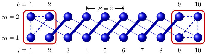 Figure 2
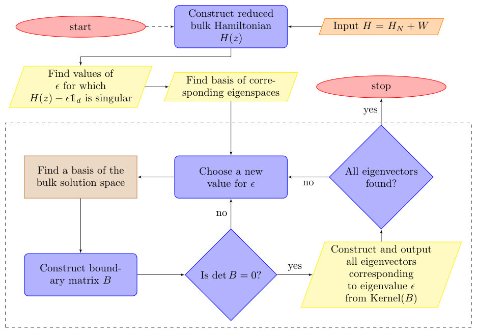 Figure 3
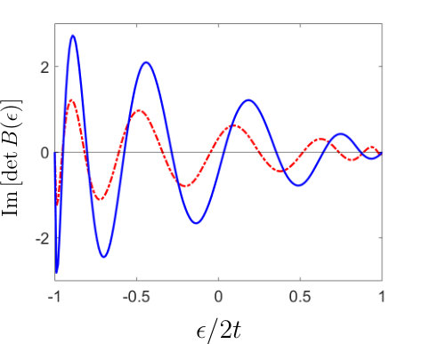 Figure 4
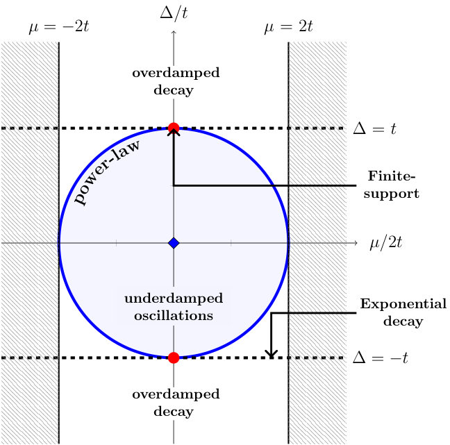 Figure 5
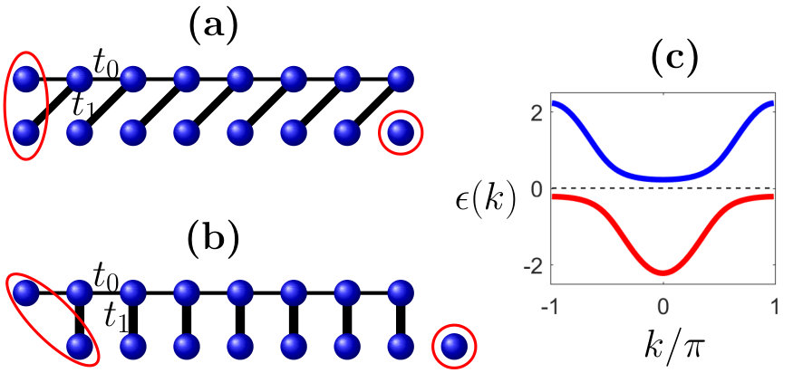 Figure 6
 Figure 7
 Figure 8
Peer Reviews
No public reviews on file for this paper yet. If you reviewed it on a platform where reviews are public (OpenReview, ICLR, NeurIPS, ICML), you can paste yours below so the community can read it here.
Videos
No videos yet. Explain this paper in a talk, walkthrough, or lecture? Add one.
A generalization of Bloch’s theorem for arbitrary boundary conditions:
Theory
Abhijeet Alase
Department of Physics and Astronomy, Dartmouth College, 6127 Wilder Laboratory, Hanover, New Hampshire 03755, USA
Emilio Cobanera
Department of Physics and Astronomy, Dartmouth College, 6127 Wilder Laboratory, Hanover, New Hampshire 03755, USA
Gerardo Ortiz
Department of Physics, Indiana University, Bloomington, Indiana 47405, USA
Department of Physics, University of Illinois, 1110 W Green Street, Urbana, Illinois 61801, USA
Lorenza Viola
Department of Physics and Astronomy, Dartmouth College, 6127 Wilder Laboratory, Hanover, New Hampshire 03755, USA
Abstract
We present a generalization of Bloch’s theorem to finite-range lattice systems of independent fermions, in which translation symmetry is broken solely due to arbitrary boundary conditions, by providing exact, analytic expressions for all energy eigenvalues and eigenstates. Starting with a re-ordering of the fermionic basis that transforms the single-particle Hamiltonian into a corner-modified banded block-Toeplitz matrix, a key step is a Hamiltonian-dependent bipartition of the lattice, which splits the eigenvalue problem into a system of bulk and boundary equations. The eigensystem inherits most of its solutions from an auxiliary, infinite translation-invariant Hamiltonian that allows for non-unitary representations of translation – hence complex values of crystal momenta with specific localization properties. A reformulation of the boundary equation in terms of a boundary matrix ensures compatibility with the boundary conditions, and determines the allowed energy eigenstates in the form of generalized Bloch states. We show how the boundary matrix quantitatively captures the interplay between bulk and boundary properties, leading to the construction of efficient indicators of bulk-boundary correspondence. Remarkable consequences of our generalized Bloch theorem are the engineering of Hamiltonians that host perfectly localized, robust zero-energy edge modes, and the predicted emergence, for instance in Kitaev’s Majorana chain, of localized excitations whose amplitudes decay in space exponentially with a power-law prefactor. We further show how the theorem may be used to construct numerical and algebraic diagonalization algorithms for the class of Hamiltonians under consideration, and use the proposed bulk-boundary indicator to characterize the topological response of a multi-band time-reversal invariant -wave topological superconductor under twisted boundary conditions, showing how a fractional Josephson effect can occur without entailing a fermionic parity switch. Finally, we establish connections to the transfer matrix method and demonstrate, using the paradigmatic Kitaev’s chain example, that a defective (non-diagonalizable) transfer matrix signals the presence of solutions with a power-law prefactor.
I Introduction
Modern electronic transport theory in crystalline solids relies on two fundamental tenets. On the one hand, because of the Pauli exclusion principle, electrons satisfy Fermi-Dirac statistics; on the other, Bloch’s theorem allows labeling of the one-electron wave-functions in terms of their crystal momenta. The set of allowed momenta, defining the so-called Brillouin zone, is determined by symmetry and the fact that Born-von-Karman (periodic) boundary conditions (BCs) are enforced on the systemashcroftmermin . It is the organization of electrons within the Brillouin zone that is key to defining its conduction properties. While the assumption of a perfect crystal with a unit cell that is periodically repeated emphasizes the (discrete) symmetry of translation, the torus topological constraint imposed by the Born-von-Karman condition further eliminates the potential emergence of edge or boundary electronic states in a real, finite crystal. Although much of the transport properties are determined by bulk electrons, technologically relevant processes on the surface of solids are known to lead to intriguing phenomena, such as surface superconductivity gor'kov or Kondo screening of magnetic impurities resulting in exotic surface spin textures kondoleonid . Early theoretical investigations by Tamm and Shockley Tamm ; Shockley initiated the systematic study of surface state physics, that witnessed a landmark achievement with the discovery of the quantum Hall effect hall , and that today finds its most striking applications in topological insulating and superconducting materials bernevig .
The organization of bulk electrons comes with a twist. The quantum electronic states labeled by crystal momenta organize in ways subject to classification according to integer values of topological invariants defined over the entire Brillouin zone zak ; chiu16 . The first Chern number, determined in terms of the Berry connection, is one of those topological invariants, defining a topologically non-trivial electronic phase whenever its value differs from zero bernevig . For instance, the transverse conductivity of a quantum Hall fluid is proportional to such a Chern number. Perhaps surprisingly, there appears to be a connection between a non-vanishing value of the topological invariant, a bulk property, and the emergence of “robust” boundary states, an attribute of the surface. This principle is known as the bulk-boundary correspondence bernevig ; Graf13 ; chiu16 . At first, this relation seems odd, since surface properties are totally independent from those of the bulk; for example, one can deposit impurities, generate strain and reconstruction, or add externally applied electric fields only on the surface. Nonetheless, it seems reasonable to assume that as long as the symmetry protecting the surface states is not broken by external means, a bulk-boundary correspondence will still hold, although the quantum surface state will, in general, get transformed isaev11 . In other words, although the mere existence of a boundary mode may be robust, only classical information may be protected in general isaev11 ; ips .
It is apparent that Bloch’s theorem and its consequences pertain to the realm of bulk physics. A crystal without boundaries is required to establish it. But, can one generalize Bloch’s theorem for independent electrons to arbitrary BCs, so that bulk and surface states can be handled on an equal footing, and physical insight about the interplay between bulk and boundary may be gained? In light of our previous discussion, it is clear that to accomplish such a task one needs to give up on some concepts, such as the notion of a Brillouin zone. If possible, such a generalization would allow us to formulate a bulk-boundary correspondence principle that makes use of both bulk and boundary information. It is tempting to argue that the relative importance of BCs diminishes as the size of the crystal grows. Notwithstanding, for example, recent work shows that BCs impact the quasi-conserved local charges of one-dimensional systems, with important consequences for bulk quench dynamics fagotti ; gluza16 . More generally, the statistical mechanics of topologically nontrivial systems begs some answers directly relevant to the questions above quelle15 ; quelle16 .
In this paper, we generalize Bloch’s theorem to systems of independent electrons subject to arbitrary BCs. Intuitively speaking, one may expect such a result on the basis that translation symmetry is only mildly broken by BCs – namely, clean (disorder-free) systems are translationally-invariant away from the boundary. Our generalized Bloch theorem makes this idea precise, by providing an exact (often in fully closed-form) description of the eigenstates of the system’s Hamiltonian in terms of generalized eigenstates of non-unitary representations of translation symmetry in infinite space, that is, with boundaries at infinity and no torus topology commentAM . As a result, both exponentially decaying edge modes and more exotic modes with power-law prefactors can emerge, provided the BCs allow them. Our generalized Bloch theorem leverages the bulk-boundary separation of the Schrödinger equation we introduced in Ref. [abc, ] and the full solution of the bulk equation rigorously established in Ref. [JPA, ]. It extends the diagonalization procedure described in Ref. [abc, ], and recently used in Ref. [KatsuraTwisted, ], to a more general class of Hamiltonians and BCs, which in particular allows for different modifications to be imposed on different boundaries. A unifying theme behind these results is an effective analytic continuation to the complex plane of the standard Bloch’s Hamiltonian off the Brillouin zone. This analytic continuation is remarkably useful because the original problem reduces to a matrix polynomial function JPA . Interestingly, a recent study made use of similar polynomial structures for the purpose of topological classification read16 .
The outline of this paper is as follows. In Sec. II we discuss a re-arrangement of the fermionic basis that allows us to reduce the diagonalization of the original many-electron finite-range quadratic Hamiltonian in second quantization, subject to specified BCs, to the one of a single-particle Bogoliubov-de Gennes Hamiltonian that has the structure of a corner-modified block-Toeplitz matrix, as introduced in Ref. [JPA, ]. Section III develops a structural characterization of the energy eigenstates for the many-electron systems under consideration, culminating into our generalization of Bloch’s theorem. Like the usual Bloch’s theorem, such a generalization is first and foremost a practical tool for calculations, granting direct access to exact energy eigenvalues and eigenstates. In Sec. IV, we provide two new procedures – one numerical and another algebraic – for carrying out the exact diagonalization of the single-particle Hamiltonian, based on the generalized Bloch theorem. The algebraic procedure, which may provide closed-form solutions to the problem, is explicitly illustrated through a number of examples in Sec. V. While, in order to illustrate our methodology, we focus largely on one-dimensional systems here, we anticipate that additional applications to higher-dimensional problems will be addressed in a companion paper PRB2 . Remarkably, while mid-gap modes with power-law prefactors have been predicted for systems with long-range couplings, we show analytically that they can also prominently manifest in short-range tight-binding models of topological insulators and superconductors pientka13 ; degottardi13 ; vodola14 ; ortiz14 ; yazdani14 .
Crucially, our generalized Bloch theorem also allows derivation of a boundary indicator for the bulk-boundary correspondence, which contains information from both the bulk and the BCs and, as remarked in Ref. [abc, ], is computationally more efficient than other indicators also applicable in the absence of translational symmetry kitaev01 . This is the subject of Sec. VI. In the same section, we expand on the analysis of the two-band time-reversal invariant -wave topological superconducting wire we introduced previously swavePRL ; swavePRB , by employing our newly defined indicator of bulk-boundary correspondence – constructed by using the generalized Bloch theorem, as opposed to the simplified Ansatz we presented in Ref. [abc, ]. Specifically, this indicator is employed in the analysis of the Josephson response of the -wave superconductor in a bridge configuration, sharply diagnosing the occurrence of a fractional -periodic Josephson effect. Remarkably, we find that this is possible without a conventional fermionic parity switch, which we explain based on a suitable transformation into two decoupled systems, each undergoing a parity switch. Section VII establishes some important connections between our generalized Bloch theorem and the widely employed transfer matrix approach Lee . Interestingly, from the standpoint of computing energy levels, our bulk-boundary separation is in many ways complementary to the transfer matrix method. While the latter can handle bulk disorder (at a computational cost), it does not, a priori, lend itself to investigating the space of arbitrary BCs in a transparent way. On the contrary, our generalized Bloch theorem can handle arbitrary BCs efficiently, as long as the bulk respects translational invariance – with arbitrary (finite-range) disorder on the boundary being permitted. Looking afresh at the transfer matrix approach from the generalized Bloch theorem’s perspective yields a remarkable result: the generalized eigenvectors of the transfer matrix, whose role has been appreciated only recently DwivediBB , describe energy eigenstates with power-law corrections to an otherwise exponential behavior. Our generalized Bloch theorem further suggests a way to extend the transfer matrix approach to a disordered bulk and arbitrary BCs. A discussion of the main implications of our work, along with outstanding research questions, concludes in Sec. VIII, whereas additional technical material is included in separate appendixes.
II From independent fermions to Toeplitz matrices
We begin by describing the class of model Hamiltonians investigated in this and the companion paper PRB2 . The upshot of this section will be a non-conventional re-ordering of the physical subsystems’ labels that allows recasting the single-particle (Bogoliubov-de Gennes (BdG)) Hamiltonians in Toeplitz form, essential for the exact diagonalization procedure we will describe.
Consider a -dimensional, translation-invariant infinite system of independent fermions. Such a system is described in full generality by a quadratic, not necessarily particle-number-conserving, Hamiltonian in Fock space. In a lattice approximation, the vector position of a given fermion in the regular crystal lattice can be written as the sum of a Bravais lattice vector and a basis vector ashcroftmermin . We will include these basis vectors as part of the internal labels, and denote Bravais lattice vectors as , with primitive vectors and each . An orthonormal basis of the Hilbert space of single-particle states is thus labeled by Bravais lattice vectors , and a finite number of internal labels . We denote by () the fermionic annihilation (creation) operator corresponding to lattice vector and internal state . The Hamiltonian of a translation-invariant system can then be written as
[TABLE]
with , a Bravais lattice vector, and the hopping and pairing matrices , satisfying , where the superscript denotes the transpose operation. For arrays, such as and , we stick to the convention that those appearing on the left (right) of a matrix are row (column) arrays.
Since the infinite system is translation-invariant in all directions, it is customary to introduce the volume containing the electrons by imposing Born-von Karman (periodic) BCs over a macroscopic volume commensurate with the primitive cell of the underlying Bravais lattice. If the allowed ’s in the macroscopic volume correspond to , then,
[TABLE]
defines the Fourier-transformed array of creation operators of real Bloch wavevector (or crystal momentum), , with integers such that lies inside the Brillouin zone. The total number of primitive cells is given by , and defines the reciprocal lattice vectors satisfying , with representing Kronecker’s delta ashcroftmermin . Finally, by letting denote complex conjugation, one can express the Hamiltonian of Eq. (1) in momentum space as
[TABLE]
which has a block structure in terms of the matrices
[TABLE]
Now let us turn our attention to systems that are periodic along directions and terminated by two parallel hyperplanes perpendicular to the direction . We then write the allowed values of as
[TABLE]
In this scenario, each Bloch wavevector is no longer a good quantum number. However, we can still block-diagonalize the Hamiltonian in the partial basis
[TABLE]
where is defined to be the array
[TABLE]
A system with sudden termination at hyperplanes correspondig to and is modeled by open (or hardwall) BCs, in which case the Hamiltonian can be expressed as ,
[TABLE]
in terms of matrices
[TABLE]
and analogously defined matrices . We will henceforth assume that the range of hopping and pairing along the direction is finite. This means that
[TABLE]
In this paper, we are interested in BCs more general than open BCs. They are modeled by a Hermitian many-body operator on Fock space which satisfies the following restrictions (see also Appendix A):
- •
has no effect beyond the “boundary slab”, containing basis vectors
[TABLE]
- •
is periodic along the directions , and has a decomposition analogous to that of .
Because of the latter restriction, with
[TABLE]
where , is Hermitian and is antisymmetric for each . Then, the model Hamiltonian, with arbitrary BCs, becomes
[TABLE]
From now on, we will focus on diagonalizing one such block , for a fixed value of . We will investigate the interplay between and our diagonalization algorithm, (and, more generally, disordered BCs), in Ref. [PRB2, ].
The next step consists of deriving the BdG Hamiltonian for this block. The conventional way blaizot is to use the (Nambu) basis , with defined in Eq. (2), so that can be expressed in the form,
[TABLE]
in terms of a Hermitian matrix (note that the matrix has entries if any of take values from the set ). This relation leads us to a BdG Hamiltonian with
[TABLE]
The diagonalization of the BdG Hamiltonian implies that of , as detailed for example in Ref. [blaizot, ].
The block-structure of emphasizes the intrinsic charge-conjugation symmetry under the anti-unitary operator , i.e., where is the Pauli -matrix in the Nambu basis, and denotes complex conjugation. Such a block-structure, however, does not explicitly highlight the role of translation invariance. For this reason, we reorder the (Nambu) basis according to abc
[TABLE]
so that the BdG Hamiltonian transforms to
[TABLE]
in terms of a banded block-Toeplitz matrix , with entries along the diagonals, and a block matrix , where
[TABLE]
[TABLE]
Explicitly, in array form, we have:
[TABLE]
[TABLE]
where we have used the notation
[TABLE]
Here, the superscript [or ] indicates the entries that allow hoppings only near the left [or right] boundary, whereas the ones without superscript allow hoppings from the left to the right boundary slabs. The matrix is a corner-modified banded block-Toeplitz matrix as defined in Ref. [JPA, ], and is amenable to the exact solution approach described therein RemarkSymm .
This transformed BdG Hamiltonian allows us to write the second-quantized Hamiltonian in the form
[TABLE]
where we have dropped the label everywhere. In particular, for one-dimensional systems (=1), we recover (up to a constant) the class of Hamiltonians considered in Ref. [abc, ], provided that is expressible as
[TABLE]
for some matrices .
Notice that for particle number-conserving systems (), the single-particle Hamiltonian is just , which is already a corner-modified, banded block-Toeplitz matrix. In such cases, the re-ordering of the basis is not required, and one may directly apply the diagonalization procedure described in the following sections to , with internal blocks of dimension . In order to have a uniform notation, we shall use
[TABLE]
III Algebraic characterization of energy eigenstates
A main goal of this work is to diagonalize the single-particle Hamiltonian , which is a corner-modified, banded block-Toeplitz matrix. In this section, we investigate the structure of its energy eigenstates, which will culminate in a generalization of Bloch’s theorem to systems described by such model Hamiltonians. Our analysis will illustrate, in particular, that for non-generic parameter values, Hamiltonians may display a finite number of exceptional (singular) energies corresponding to dispersionless, flat bands. The latter represent a macroscopic number of energy eigenstates that are localized in the bulk and, thus, are completely insensitive to BCs. It is remarkable that the analytic continuation of the Bloch Hamiltonian can still encompass this situation. We will show how to use it to construct the localized flat band energy eigenstates directly in real space.
III.1 An impurity problem as a motivating example
Consider the simple tight-binding Hamiltonian
[TABLE]
defined on an open chain of (even) lattice sites with nearest-neighbor hopping strength , and lattice constant . The corresponding single-particle Hamiltonian is
[TABLE]
and breaks translation-invariance due to the presence of the boundary, so that the crystal momentum is not a good quantum number. In fact, for any , the state (labeled by ) obeys
[TABLE]
with a similar relation holding for
[TABLE]
The first term on the right-hand side of Eqs. (7)-(8) indicates that and “almost” (for large ) satisfy the eigenvalue relation with energy , while the two terms in the brackets show that the eigenvalue relation is violated near the two edges of the chain. Under periodic BCs, is the actual energy eigenvalue of the eigenstate (and ), and is the crystal momentum, given by ashcroftmermin .
Because of the identical first term in Eqs. (7) and (8), the states and can be linearly combined in order to cancel off the similar-looking boundary contributions. For , the eigenvalue relation
[TABLE]
is recovered provided that the constraint
[TABLE]
is satisfied. For this to hold, the coefficients of both and must vanish, which leads to the kernel equation
[TABLE]
The determinant of the above “boundary matrix” must vanish, which happens if the condition is satisfied, that is, when . For each of these values of , provides the required kernel vector of the boundary matrix, with the resulting eigenvectors
[TABLE]
of energy . Notice that the allowed values of differ from the case of periodic BCs Mikeska .
Encouraged by these results, let us change the Hamiltonian by adding an on-site potential at the edges,
[TABLE]
so that the total single-particle Hamiltonian becomes . The boundary matrix changes to
[TABLE]
While it is harder to predict analytically the values of for which it has a non-trivial kernel, it is interesting to examine the limit . Then, we can approximate the relevant kernel condition as
[TABLE]
showing nontrivial solutions if . There are now -values yielding stationary eigenstates as before. The two missing eigenstates are localized at the edges, and can be taken to be and , to leading order in . These localized states are reminiscent of Tamm-Shockley modes Tamm ; Shockley .
In hindsight, it is natural to ask whether this approach to diagonalization may be improved and extended to more general Hamiltonians. The answer is Yes, and this paper provides the appropriate tools.
III.2 The bulk-boundary system of equations
The above motivating example suggests that it may be possible to isolate the extent to which boundary effects prevent bulk eigenstates from becoming eigenstates of the actual Hamiltonian. Consider Eqs. (7) and (8) in particular. We may condense them into a single relative eigenvalue equation, in terms of the projector The extension of this observation to the general class of Hamiltonians requires only knowledge of the range in Eq. (4). The block-structure of defines a subsystem decomposition of the single-particle state space abc ,
[TABLE]
where and are lattice and internal state spaces of dimensions and , respectively. Let and be their respective orthonormal bases. Define bulk and boundary projectors,
[TABLE]
with the identity matrix on , and , the identity matrices on and respectively (see Fig. 1). The defining property of the bulk projector is that it annihilates any boundary contribution , that is, . Because , the bulk-boundary system of equations,
[TABLE]
may be seen to be completely equivalent to the standard eigenvalue equation, JPA .
This bulk-boundary separation of the eigensystem problem is advantageous because the bulk equation is, in a well-defined sense, translation-invariant. Let us define a left-shift operator on the lattice space (see Appendix B). Then, one may verify that
[TABLE]
By extending infinitely on both directions, we obtain a translation-invariant auxiliary Hamiltonian,
[TABLE]
where now denotes the generator of discrete translations on the (infinite-dimensional) vector space spanned by , and the corresponding identity operator. The subtle difference between Hamiltonians and is that while is not invertible, is, and in fact . This difference is decisive in solving the corresponding eigenvalue problems. On the one hand, the eigenvalue equation is equivalent to the infinite system of linear equations
[TABLE]
where On the other, the bulk equation , with is equivalent to Eq. (15) but restricted to the finite domain . Hence, the bulk equation is underdetermined (there are more vector variables than constraints). In particular, if is an eigenstate of the infinite Hamiltonian as above, then
[TABLE]
is a solution of the bulk equation. It is in this sense of shared solutions with that the bulk equation is, as anticipated, translation-invariant.
III.3 Exact solution of the bulk equation
Let us revisit the energy eigenvalue equation, Eq. (15). If the goal were to diagonalize the infinite-system Hamiltonian , then one should focus on finding energy eigenvectors associated to normalized states in Hilbert space. However, our model systems are of finite extent, and we are only interested in using as an auxiliary operator for finding the translation-invariant solutions of the bulk equation. Hence, we will allow to act on arbitrary vector sequences of the form possibly “well outside” the Hilbert state space, and so we will drop Dirac’s ket notation. From the standpoint of solving the bulk equation, every sequence that satisfies is acceptable, so one must find them all. In the space of all sequences, the translation symmetry remains invertible but is no longer unitary, because the notion of adjoint operator is not defined. This is important, because it means that translations need not have their eigenvalues on the unit circle, or be diagonalizable. Nonetheless, , and so both features have interesting physical consequences for finite systems.
We will refer to the space of solutions of the bulk equation as the bulk solution space and denote it by
[TABLE]
for any fixed energy . Let denote the space of eigenvectors of of energy within the space of all sequences. In terms of these spaces, our arguments in Sec. III.2 establish the relation
[TABLE]
where we dropped the argument . Translation invariance is equivalent to the properties and footnote2 . If the matrix is invertible, Eq. (16) becomes JPA .
Since commutes with , the generator of translations to the right, these two symmetries share eigenvectors of the form with an arbitrary non-zero complex number and any internal state: there are linearly independent eigenvectors of translations for each . As a simple but important consequence of the identities
[TABLE]
one finds that
[TABLE]
where the linear operator
[TABLE]
acts on the internal space only. This is precisely the reduced bulk Hamiltonian of Ref. [abc, ], obtained here by way of a slightly different argument. Since is the usual Bloch Hamiltonian of a one-dimensional system with Born-von-Karman BCs, is the analytic continuation of off the Brillouin zone.
One can similarly continue the energy dispersion relation off the Brillouin zone, by relating to via
[TABLE]
In practice, it is advantageous to use the polynomial
[TABLE]
We will say that is regular if is not the zero polynomial, and singular otherwise. That is, identically for all if is singular. Such a (slight) abuse of languageJPA is permitted since we are interested in varying for a fixed Hamiltonian. For any given Hamiltonian of finite range , there are at most a finite number of singular energies. Physically, singular energies correspond to flat bands, as one can see by restriction to the Brillouin zone. We can now state a first useful result, whose formal proof follows from the general arguments in Ref. [JPA, ]:
Theorem 1. If is regular, the number of independent solutions of the bulk equation is , for any system size .
This result ties well with the physical meaning of the number as counting the total number of degrees of freedom on the boundary, which is equal to the dimension of the boundary subspace. The condition implies that the system is big enough to contain at least one site in the bulk.
III.3.1 Extended-support bulk solutions at regular energies
The solutions of the bulk equation that are inherited from have non-vanishing support on the full lattice space , and are labeled by the eigenvalues of , possibly together with a second “quantum number” that appears because is not unitary on the space of all sequences. For any , if satisfies the eigenvalue equation then Eq. (17) implies that is an eigenvector of with eigenvalue . In order to be more systematic, let denote the distinct non-zero roots of Eq. (19), and their respective multiplicities. For generic values of , has exactly eigenvectors in , satisfying
[TABLE]
Since the states
[TABLE]
are solutions of the bulk equation. Intuitively, these states are “eigenstates of the Hamiltonian up to BCs.”
For a few isolated values of , can have less than eigenvectors. However, the number of eigenvectors of is still JPA , as we illustrate here by example. Suppose for concreteness that
[TABLE]
Since and , we expect two eigenvectors for each value of . One concludes that the eigenspace of energy is spanned by the sequences if . But, if , then , and
[TABLE]
How can one get two independent solutions in this case? The answer is that, in addition to , the factor contributes another sequence to the kernel of , namely, There are two eigenvectors in total, even though there is only one root.
Returning to the general case, the sequences JPA ; normalization
[TABLE]
span the kernel of for . In other words, is a generalized eigenvector of the translational symmetry of rank with eigenvalue . We refer to eigenvectors with as the power-law solutions of the bulk equation (solutions with a power-law prefactor). They exist because translations are not diagonalizable in the full space of sequences (as opposed to the Hilbert space of square-summable sequences), leading to the new quantum number .
The power-law solutions of the bulk equation may be found from the action of on the generalized eigenvectors of . For arbitrary internal state , we have:
[TABLE]
Then one can show from Eqs. (21) and (22) that the action of on the vector sequence , where are arbitrary internal states, is given by
[TABLE]
Here, is an upper triangular block-Toeplitz matrix with non-trivial blocks
[TABLE]
In matrix form, by letting , we have
[TABLE]
We refer to as the generalized reduced bulk Hamiltonian of order . Notice that . In the partial basis
[TABLE]
organized as a row vector, the entries of are the vector-valued coordinates of , Then, Eq. (23) can be rewritten as
[TABLE]
Now it becomes clear that for to be an eigenvector of , the required condition is , which is analogous to the condition derived for the generic case . If a root of Eq. (18) has multiplicity , then has precisely linearly independent eigenvectors corresponding to . This provides a characterization of the eigenstates of , which may be regarded as extending Bloch’s theorem to viewed as a linear transformation on the space of all vector-valued sequences, and whose rigorous justification follows from Ref. [JPA, ]:
Theorem 2. For fixed, regular , let denote the distinct non-zero roots of Eq. (18), with respective multiplicities . Then, the eigenspace of of energy is a direct sum of vector spaces spanned by generalized eigenstates of of the form
[TABLE]
where the linearly independent vectors are chosen in such a way that , and .
Once the eigenvectors of are calculated, the bulk solutions of extended support are readily obtained by projection. Let, for ,
[TABLE]
be the projections of generalized eigenvectors of . Then
[TABLE]
describes a basis of the translation-invariant solutions of the bulk equation, where
[TABLE]
Remark.— The bulk equation bears power-law solutions only at a few isolated values of Trench85 . However, linear combinations of solutions show power-law-like behavior, as soon as two or more of the roots of Eq. (18) are sufficiently close to each other. Suppose, for instance, that for some value of energy , two of the roots of Eq. (18) coincide at . For energy differing from by a small amount , the double root bifurcates into two roots slightly away from each other, with values . The relevant bulk solution space is spanned by
[TABLE]
showing that the second vector has indeed a close resemblance to the power-law solution . Similar considerations apply if , as it is typically the case in physical applications. Assuming that the relevant bulk solutions at energy are described by analytic vector functions and , then, from the above analysis, it is clear that for energy , the power-law bulk solution will be proportional to
[TABLE]
We will make use of this observation for the calculation of power-law solutions in Sec. V.2.
III.3.2 Emergent solutions at regular energies
While the extended solutions of the bulk equation correspond to the nonzero roots of Eq. (18), the polynomial defined in Eq. (19) may also include as a root of multiplicity , that is, we may generally write
[TABLE]
However, does not describe any state of the system. This observation suggests that the extended solutions of the bulk equation may fail to account for all solutions we expect for regular . That this is indeed the case follows from a known result in the theory of matrix polynomials teran15 , implying that for matrix polynomials associated to Hermitian Toeplitz matrices JPA . Hence, the number of solutions of the bulk equation of the form given in Eq. (26) is
[TABLE]
We call the missing solutions of the bulk equation emergent, because they are no longer controlled by and (nonunitary) translation symmetry, but rather they appear only because of the truncation of the infinite lattice down to a finite one, and only if JPA . Emergent solutions are a direct, albeit non-generic, manifestation of translation-symmetry-breaking; nonetheless, remarkably, they can also be determined by the analytic continuation of the Bloch Hamiltonian, in a precise sense.
While full technical detail is provided in Appendix C, the key to computing the emergent solutions is to relate the problem of solving the bulk equation to a half-infinite Hamiltonian, rather than the doubly-infinite we have exploited thus far. Let us define the unilateral shifts
[TABLE]
The Hamiltonian
[TABLE]
is then the half-infinite counterpart of . The corresponding half-infinite bulk projector is
[TABLE]
Suppose there is a state , that solves the equation Then one can check that is a solution of the bulk equation, Eq. (12). Clearly, some of the bulk solutions we arrive at in this way using will coincide with those obtained from . These are precisely the extended solutions we already computed in Sec. III.3.1. In contrast, the emergent solutions are obtained only from .
Since , we may write in terms of the matrix polynomial
[TABLE]
Half of the emergent solutions, namely, the ones localized on the left edge, are determined by the kernel of , with constructed as in Eq. (24). Explicitly, such a matrix, which was obtained by different means in Ref. [JPA, ], takes the form
[TABLE]
for systems with fairly large . Let denote a basis of the kernel of , with
[TABLE]
Then,
[TABLE]
are the emergent solutions with support on the first lattice sites, with obeying Eq. (28).
We are still missing emergent solutions for the right edge. They may be constructed from the kernel of the lower-triangular block matrix Let denote a basis of the kernel of , with
[TABLE]
Then,
[TABLE]
are the emergent bulk solutions associated to the right edge, supported on the lattice sites . Again, for mathematical justifications, see Appendix C.
In what follows, we shall denote the spaces spanned by left- and right- localized emergent bulk solutions by and , and their bases by and , respectively.
III.3.3 Bulk-localized states at singular energies
If is not invertible, there can be at most a finite number of singular energy values (usually referred to as flat bands), leading to bulk-localized solutions: these solutions are finitely-supported and appear everywhere in the bulk. Hence, a singular energy cannot be excluded from the physical spectrum of a finite system by way of BCs. In contrast, emergent solutions are also finitely-supported but necessarily “anchored” to the edges (and only appearing for regular values of ).
Recall that if is singular, then for any . Thus, there exists an analytic vector function,
[TABLE]
satisfying for all . To obtain , one can construct the adjugate matrix of . (Recall that the adjugate matrix associated to a square matrix is constructed out of the signed minors of and satisfies .) Hence,
[TABLE]
and so one can use any of the non-zero columns of , suitably pre-multiplied by a power of , for the vector polynomial . By matching powers of , this equation becomes
[TABLE]
The idea now is to use the linearly independent solutions of Eq. (35) to construct finite-support solutions of the bulk equation. Let us denote such solutions by , for . One can check directly that the finitely-supported sequences
[TABLE]
all satisfy because obeys Eq. (35). Hence, the states provide finitely-supported solutions of the bulk equation. In addition, as long as , the boundary equation is also satisfied trivially, and so all such states become eigenvectors of with the singular energy . This is why singular energies, if present for the infinite system, are necessarily also part of the spectrum of the finite system and display macroscopic degeneracy of order .
Let us further remark that the sequences and associated solutions of the bulk equation need not be linearly independent. To obtain a complete (rather than overcomplete), set of solutions for flat bands, one would require a technical tool, the Smith normal form Gohberg , which is beyond the scope of this paper. See Ref. [JPA, ] for details.
III.4 The boundary matrix
For regular energies, the bulk solutions determine a subspace of the full Hilbert space [Theorem 1], whose dimension for typical applications. While not all bulk solutions are eigenstates of the Hamiltonian , the actual eigenstates must necessarily appear as bulk solutions. Hence, the bulk-boundary separation in Eqs. (12), and, in particular, the bulk equation, identifies by way of a translational symmetry analysis a small search subspace. In order to find the energy eigenstates efficiently, one must solve the boundary equation on this search subspace. Since the boundary equation is linear, its restriction to the space of bulk solutions can be represented by a matrix, the boundary matrix abc . The latter is a square matrix that combines our basis of bulk solutions with the relevant BCs.
Let be a basis for . Then, building on the previous section, the Ansatz state
[TABLE]
represents the solutions of the bulk equation parametrized by the amplitudes , where
[TABLE]
Moreover, let as before label the boundary sites. Then,
[TABLE]
In particular, the boundary equation is equivalent to the requirement that for all boundary sites. Since denotes a row array of internal states, it is possible to organize these arrays into the boundary matrix
[TABLE]
By construction, the boundary matrix is a block matrix of block-size . In terms of this matrix, Eq. (40) provides the useful identity
[TABLE]
One may write an analogous equation in Fock space by defining an array
[TABLE]
Then Eq. (42) translates into
[TABLE]
It is interesting to notice that this (many-body) relation remains true even if is allowed to be a complex number.
III.5 The generalized Bloch theorem
The bulk-boundary separation of the energy eigenvalue equation shows that actual energy eigenstates are necessarily linear combinations of solutions of the bulk equation. This observation leads to a generalization of Bloch’s theorem for independent fermions under arbitrary BCs:
Theorem 3 (Generalized Bloch theorem). Let denote the single-particle Hamiltonian of a clean system subject to BCs described by . If is a regular energy eigenvalue of of degeneracy , the associated eigenstates can be taken to be of the form
[TABLE]
where is a basis of the kernel of the boundary matrix at energy .
In short, if and only if , in which case it also follows from Eq. (43) that is a normal fermionic mode of the many-body Hamiltonian . From now on, we will refer to energy eigenstates of the form as generalized Bloch states. Recall that acts on , with couplings of finite range . A lower bound on should be obeyed, in order for the above theorem to apply. If , since there are no emergent solutions nor flat bands, generalized Bloch states describe the allowed energy eigenstates as soon as , independently of . If fails to be invertible, we should require that to ensure that emergent solutions on opposite edges do not overlap, and are thus independent. Since , this condition is satisfied for any . In general, always suffices for generalized Bloch states to describe generic energy eigenstates JPA .
We further note that if is not an energy eigenvalue, the kernel of is trivial. Thus, the degeneracy of a single-particle energy level coincides with the dimension of the kernel of . Let denote the single-particle density of states. Combining its definition with the generalized Bloch theorem, we then see that
[TABLE]
an alternative formula to the usual
[TABLE]
from the theory of Green’s functions ballentine . Another interesting and closely related formula is
[TABLE]
for the partition function of the single-particle Hamiltonian, with the dependence on BCs highlighted quelle15 .
We conclude this section by showing how, for periodic BCs, one consistently recovers the conventional Bloch’s theorem. In this case, the appropriate matrix reads
[TABLE]
since then one can check that
[TABLE]
in terms of the fundamental circulant matrix
[TABLE]
Physically, is the generator of translations (to the left) for a system displaying ring (1-torus) topology.
The Bloch states are the states that diagonalize and simultaneously. Theorem 3 guarantees that we can choose the eigenstates of to be linear combinations of translation-invariant and emergent solutions. Thus, we only need to check if these linear combinations include eigenstates of . There is no hope of retaining the emergent solutions, because they are localized and too few in number (at most ) to be rearranged into eigenstates of . The same holds for translation-invariant solutions with a power-law prefactor. Hence, the search subspace that is compatible with the translational symmetry is described by the simplified Ansatz abc
[TABLE]
Now, and so the generalized Bloch states can only be eigenstates of if with , and all but one entry in vanish. That is, As one may verify, showing that is indeed compatible with the boundary matrix. Manifestly, is an eingenstate of in the standard Bloch form – thereby recovering the conventional Bloch’s theorem for periodic BCs, as desired.
IV The bulk-boundary algorithms
The results of Sec. III can be used to develop diagonalization algorithms for the relevant class of single-particle Hamiltonians. We will describe two such algorithms. The first treats as a parameter for numerical search. The second is inspired by the algebraic Bethe Ansatz, as suggested by comparing our Eq. (42) to Eq. (28) of Ref. [ortiz05, ].
IV.1 Numerical “scan-in-energy” diagonalization
The procedure described in this section is a special instance of the Eigensystem Algorithm described in Ref. [JPA, ], specialized to Hermitian matrices. It employs a search for energy eigenvalues along the real line, and takes advantage of the results of Sec. III to determine whether a given number is an eigenvalue. The overall procedure is schematically depicted in Fig. 2.
The first part of the algorithm finds all eigenvectors of that correspond to the flat (dispersionless) energy band, if any exists. Two steps are entailed:
Find all real values of for which vanishes for any . Output these as singular eigenvalues of . 2. 2.
For each of the eigenvalues found in step (1), find and output a basis of the corresponding eigenspace of using any conventional algorithm.
In implementing step (2) above, one can leverage the analysis of Sec. III.3.3. The following part of the algorithm, which repeats until all eigenvectors of are found, proceeds according to the following steps:.
Choose a seed value of , different from those eigenvalues found already. 2. 4.
Find all distinct non-zero roots of the equation . Let these roots be , and their respective multiplicities . 3. 5.
For each such roots, construct the generalized reduced bulk Hamiltonian [Eq. (24)]. 4. 6.
Find a basis of the eigenspace of with eigenvalue . Let the basis vectors be . The bulk solution corresponding to is , with defined in Eq. (25). 5. 7.
If is non-invertible, find . Construct matrices as described in Eq. (III.3.2), and . 6. 8.
Find bases of the kernels of and . Let the basis vectors be and , respectively. The emergent bulk solutions corresponding to each are follow from Eqs. (32) and (33). 7. 9.
Construct the boundary matrix [Eq. (41)]. 8. 10.
If , output as an eigenvalue. Find a basis of the kernel of . Then a basis of the eigenspace of corresponding to energy is , with being defined in Eqs. (39). If all eigenvectors are not yet found, then go back to step (3). 9. 11.
If , choose a new value of as dictated by the relevant root-finding algorithm NoteRoot . Go back to step (4).
Some considerations are in order, in regard to the fact that the determinant of plotted as a function of energy may display finite-precision inaccuracies, that appear as fictitious roots. Such issues arise at those where two (or more) of the roots of Eq. (18) cross as a function of , due to the non-orthogonality of the basis that results from the procedure described in Sec. III.3. Let be a value of energy for which this happens, so that the bulk equation bears a power-law solution. For (except itself), Eq. (18) has two roots that are very close in value, so that the corresponding bulk solutions overlap almost completely. This results in a boundary matrix having two nearly identical columns, with determinant vanishing in the limit , irrespective of being an eigenvalue of (hence, a physical solution). However, if we calculate exactly at , then the basis contains power-law solutions, and accurately indicates whether is an eigenvalue. This also means that the function has a discontinuity at .
A simple way to identify those fictitious roots is as follows. Rewrite the polynomial in Eq. (19) as
[TABLE]
which is treated as a polynomial in with coefficients depending on (if changes with , we use the smallest possible value of in Eq. (44)). has double roots at if and only if the discriminant Gelfand08 . The latter gives a polynomial expression in , of degree . By finding the roots of this equation, one can obtain all the values of for which fictitious roots of may appear. To check whether these roots are true eigenvalues, one then needs to construct by including the power-law solutions in the Ansatz.
We further note that, while the Ansatz is not continuous at such values of , the fact that the bulk solution space is the kernel of the linear operator implies that it must change smoothly with . A way to improve numerical accuracy would be to construct an orthonormal basis (e.g., via Gram-Schmidt orthogonalization) of at each , and use this basis to construct a modified boundary matrix . In practice, one may directly compute the new determinant by using
[TABLE]
where is the Gramian matrix grammatrix of the basis of bulk solutions obtained in steps (4) to (8) of the algorithm, with entries In fact, it can be checked that the bulk solutions
[TABLE]
form an orthonormal basis of the bulk solution space . The calculation of the entries of the Gramian is straightforward thanks to the analytic result
[TABLE]
In regard to the time and space complexity of the algorithm, the required resources depend entirely on those needed to compute the boundary matrix. For generic , regardless of the invertibility of , the size of is , independently of . Calculation of each of its entries is also simple from the point of view of complexity, thanks to the fact that is symmetrical RemarkSymm ; JPA . Accordingly, both the number of steps and the memory space used by this algorithm do not scale with the system size , making this approach computationally more efficient than conventional methods of diagonalization of generic Hermitian matrices Demmel07 .
IV.2 Algebraic diagonalization
The scan-in-energy algorithm can be further developed into an algorithm that yields an analytic solution (often closed-form), in the same sense as the Bethe Ansatz method does for a different class of (interacting) quantum integrable systems. The idea is to obtain, for generic values of , an analytic expression for , since its determinant will then provide a condition for to be an eigenvalue, and the corresponding eigenvectors can be obtained from its kernel. As mentioned, for generic , the extended bulk solutions do not include any power-law solutions. This property can be exploited to derive an analytic expression for in such a generic setting. The values of for which power-law solutions appear, or the analytic expression fails for other reasons, can be dealt with on a case-by-case basis.
By the Abel-Ruffini theorem, a completely closed-form solution by radicals in terms of can be achieved if the degree in of the characteristic polynomial of the reduced bulk Hamiltonian is at most four. If this is not the case, the roots do not possess an algebraic expression in terms of and entries of . The workaround is then to consider as free variables, with the constraint that each of them satisfy the characteristic equation of . With these tools in hand, the following procedure can be used to find an analytical solution for generic values of :
Construct the polynomial in Eq. (44), which is a bivariate polynomial in and . Determine using where denotes the degree of the polynomial in . 2. 2.
Assuming that and satisfy , find an expression for the eigenvector of with eigenvalue . 3. 3.
Consider variables , each satisfying . Each of these corresponds to a bulk solution . 4. 4.
If is not invertible, construct matrices and [Eq. (III.3.2)]. 5. 5.
Find bases for their kernels, each of which contains vectors. Let these be and . These correspond to finite-support solutions of the bulk equation. 6. 6.
Construct the boundary matrix [Eq. (41)]. 7. 7.
The condition for being an eigenvalue of is . Therefore, a complete characterization of eigenvalues is
[TABLE] 8. 8.
If , substitute for each the closed-form expression of the corresponding root . The eigenvalue condition in step (7) simplifies to a single equation, 9. 9.
For every eigenvalue , the kernel vector of provides the corresponding eigenvector of .
In steps (2), (5) and (9), we need to obtain an analytic expression for the basis of the kernel of a square symbolic matrix of fixed kernel dimension in terms of its entries. This can be done in many different ways, and often is possible by inspection. One possible way was described in Sec. III.3.3 in connection to evaluating Ker( for singular values of . The above analysis does not hold when satisfies any of the following conditions:
- (i)
has one or more double roots. This is equivalent to , as discussed in Sec. IV.1. This is a polynomial equation in terms of , the roots of which yield all required values of . 2. (ii)
The coefficient of in vanishes, or equivalently, is a root of . 3. (iii)
Each entry of vanishes. Such points are identified by solving simultaneously the equations and , Since a necessary and sufficient condition for these polynomials (in ) to have a common root is that their resultant vanishes Gelfand08 , we find the relevant values of by equating the pairwise resultants to zero. 4. (iv)
or are linearly dependent. To find such values of , one may form the corresponding Gramian matrix and equate its determinant to zero.
For all the values of thus identified, is calculated by following steps (4)-(10) in the scan-in-energy algorithm. To summarize, this algebraic procedure achieves diagonalization in analytic form: the upshot is a system of polynomial equations, whose simultaneous roots are the eigenvalues, and an analytic expression for the eigenvectors, with parametric dependence on the eigenvalue.
V Illustrative examples
This section contains three paradigmatic examples illustrating the use of our generalized Bloch theorem, along with the resulting algebraic procedure of diagonalization.
V.1 The impurity model revisited
Let us first reconsider the impurity model of Sec. III.1. The single-particle Hamiltonian is the corner-modified, banded block-Toeplitz matrix , with
[TABLE]
The boundary consists of two sites, so that , for any . Likewise, . The first step in diagonalizing is solving the bulk equation. Since the reduced bulk Hamiltonian ,
[TABLE]
Thus, every value of is regular and yields two ( the number of boundary degrees of freedom) solutions of the bulk equation. If , the solutions are , with
[TABLE]
with and . The special values for which yields only one of the two bulk solution have an interpretation as the edges of the energy band. If , then yields only , whereas if , it yields only . In order to obtain the missing bulk solution in each case, one must consider the effective Hamiltonian [Eq. (24)]
[TABLE]
One may check that if . Thus, the two linearly independent solutions of the bulk equation at these energies are , if , and , if .
For the purpose of solving the boundary equation, and hence the full diagonalization problem, it is convenient to organize the solutions of the bulk equation as
[TABLE]
For comparison with Sec. III.1, one should think of and . Because the Ansatz is naturally broken into three pieces, so is the boundary matrix. For instance, when , direct calculation yields
[TABLE]
However, from Eq. (45) it follows that
[TABLE]
This allows a simpler form to be obtained, by effectively changing the argument of the boundary matrix from to (or ). The complete final expression reads:
[TABLE]
Notice that if approaches , the two distinct roots collide at , and the boundary matrix becomes, trivially, a rank-one matrix, signaling the discontinuous behavior anticipated in Sec. IV.1. Furthermore, it follows from Eq. (27) that the power-law solution at may be written as . The entries of the second column of the corresponding boundary matrices satisfy , where is the double root. Thus, the entries in the second column of the boundary matrix for can be obtained by differentiating with respect to the second column of the boundary matrix for other (generic) values of , an observation we will use in other examples as well (see e.g. Sec. V.2.2). We now analyze separately different regimes (see also Fig. 3 for illustration).
V.1.1 Vanishing impurity potential
If , then and have a trivial kernel; the exotic states cannot possibly arise as physical eigenvectors. For other energies, we find that the kernel of the boundary matrix
[TABLE]
is nontrivial only if , in which case we can take and . From Eq. (45), it also follows that . Hence, there are solutions,
[TABLE]
Of the associated (un-normalized) Ansatz vectors
[TABLE]
two vanish identically ( and ). For , it is immediate to check that . This means that the Ansatz yields exactly linearly independent energy eigenvectors, of energy
[TABLE]
This is precisely the result of Sec. III.1, where the solutions were labelled in terms of allowed quantum numbers .
According to our general theory, the eigenspaces of are in one-to-one correspondence with the zeroes of . For this system then, there should be at most zeroes. The reason we find zeroes is due to the above-mentioned (quadratic) change of argument in the boundary matrix from to . Such a change of variables is advantageous for analytic work, and the associated redundancy is always rectified at the level of the Ansatz.
V.1.2 Power-law solutions
What would it take for to become eigenvectors? The kernel of is nontrivial only if
[TABLE]
These two values coincide up to corrections of order , but remember that our analysis is exact for any . Similarly, the kernel of is nontrivial only if
[TABLE]
Only one of these conditions can be met: for fixed , either is an energy eigenstate or is, but not both. Let us look more closely at the state at the bottom of the energy band. As we just noticed, this state will be a valid eigenstate for either of the two values of . Let us pick , since it yields the most interesting ground state. Then,
[TABLE]
so that one can set , , and
[TABLE]
Notice that ; that is, the power-law eigenvector of the impurity problem is an eigenstate of inversion symmetry.
V.1.3 Strong impurity potential
Lastly, consider the regime where , for large . Then, the values are excluded from the physical spectrum, and the eigenstates of the system can be determined from . We expect bound states of energy to leading order and well-localized at the edges, so that , say, with () associated to the left (right) edge. It is convenient to take advantage of this feature and modify the original Ansatz to
[TABLE]
so that () peaks at the left (right) edge, respectively. The boundary matrix becomes
[TABLE]
since . Keeping in mind that , we see that the kernel of is two-dimensional for
[TABLE]
and otherwise trivial. The corresponding energy eigenstates can be chosen to be
[TABLE]
Notice that is the mirror image of , up to normalization. The large- approach to boundary modes exemplified by the preceding calculation can be made systematic, as we will further explain in Sec. VI.1.
The remaining eigenstates consist of standing waves. They can be computed from the original boundary matrix, approximated for as
[TABLE]
This boundary matrix has a nontrivial kernel only if
[TABLE]
in which case one may choose . Then,
[TABLE]
Moreover, Hence, as needed, we have obtained linearly independent eigenvectors of energy .
The above discussion is further illustrated in Fig. 3, where the determinant of the exact boundary matrix is displayed as a function of energy.
V.2 Engineering perfectly localized
zero-energy modes: A periodic Anderson model
Having illustrated the algebraic diagonalization method on a simple impurity model, we illustrate next its usefulness toward Hamiltonian engineering. In this section, we will design from basic principles a “comb” model, see Fig. 4, with the peculiar property of exhibiting a perfectly localized mode at zero energy while all other modes are dispersive. The zero mode is distributed over two sites on the same end of the comb, with weights determined by a ratio of hopping amplitudes.
The starting point is the single-particle Hamiltonian
[TABLE]
In order to have perfectly localized eigenvectors at zero energy, the bulk equation must bear emergent solutions. Therefore, we assume that is non-invertible. Let be in the kernel of . Since annihilates ,
[TABLE]
Similarly, if is in the kernel of , then is also in the kernel of . Therefore, and are perfectly localized zero energy modes.
A concrete example may be obtained by choosing
[TABLE]
whose kernel is spanned by
[TABLE]
respectively. This example corresponds to a many-body Hamiltonian of two coupled fermionic chains, as illustrated in Fig. 4:
[TABLE]
where and denote the th fermions in the upper and lower chain, denotes intra-ladder hopping in one of the chains, and is the diagonal hopping strength between the two chains of the ladder, respectively. Physically, this “topological comb model” is closely related to the one-dimensional periodic Anderson model in its non-interacting (spinless) limit, see Ref. [Dagotto, ].
V.2.1 Zero-energy modes
The perfectly localized zero-energy modes in this case are and , that translate, after normalization, into the fermionic operators
[TABLE]
The operator trivially describes a zero-energy mode, since it corresponds to the last fermion on the lower chain, that is decoupled from the rest. However, corresponds to a non-trivial zero energy mode, localized over the first sites of the two chains. For large values of , is localized mostly on the -chain, whereas for small values it is localized mostly on the -chain.
Remarkably, such a non-trivial zero-energy mode is robust against arbitrary fluctuations in hopping strengths, despite the absence of a protecting chiral symmetry. Imagine that in Eq. (54) the hopping strengths and are position-dependent. Then, may be written as
[TABLE]
where does not contain terms involving and , so that . Then it is easy to verify that the expression for the zero-energy mode is obtained from in Eq. (55) after substituting and . We conclude that the zero-energy edge mode is protected by an “emergent symmetry”, that has a non-trivial action only on the sites corresponding to . Likewise, assume for concreteness that , and consider the inter-chain perturbation described by
[TABLE]
In this case, the corresponding single-particle Hamiltonian becomes with
[TABLE]
Nevertheless, the zero-energy mode corresponding to is still an emergent solution for , and can be verified to satisfy the boundary equation as well. The topological nature of this zero-energy mode is confirmed by its non-trivial Berry phase bernevig at half-filling. Under periodic BCs, the Hamiltonian in momentum space is
[TABLE]
leading to the following eigenvectors for the two bands:
[TABLE]
Direct calculation shows that the Berry phase has the non-trivial value , as long as .
V.2.2 Complete closed-form solution
We now obtain a complete closed-form solution of the eigenvalue problem corresponding to Eq. (54) (open BCs). The reduced bulk Hamiltonian is
[TABLE]
with the associated polynomial ()
[TABLE]
The model has two energy bands with a gap containing , and no chiral symmetry. Because is real, this enforces the symmetry of the non-zero roots of that satisfy . For generic , there are two distinct non-zero roots and, therefore, two extended bulk solutions. The eigenvector of may be generically expressed as
[TABLE]
Using Eq. (28), the number of emergent bulk solutions is , one localized on each edge. As and , such solutions are found from their kernels, spanned by and , independently of . The boundary matrix
[TABLE]
whose kernel is nontrivial only if
[TABLE]
In this case, since , we may reduce this system to one variable by substituting , which then yields the polynomial equation
[TABLE]
The algebraic system of equations (56) and (57) determine the “dispersing” extended-support bulk modes of the system. When these equations are both satisfied, the kernel of the boundary matrix is spanned by
[TABLE]
and the corresponding eigenvectors of are given by
[TABLE]
which, upon substituting , can be recast as remarkAlternative
[TABLE]
To check whether in Eq. (58) indeed satisfies the eigenvalue equation, notice that
[TABLE]
Using the expression for , vanishes trivially, while, for ,
[TABLE]
which is seen to vanish from the relation
[TABLE]
The first term on the right hand-side is equal to , whereas the second term vanishes due to Eq. (57). Finally, for , we get
[TABLE]
which equals zero, completing the argument.
Next, we find the values of for which Eq. (56) has a double root. The discriminant of is , and vanishes for and , for which the corresponding double roots are and , respectively. In these cases, the bulk equation may have power-law solutions. While one could construct the reduced bulk Hamiltonian to identify these solutions, another quick way to proceed is suggested by Eq. (27), as already remarked in Sec. V.1. A power-law solution may now be written as
[TABLE]
where is the double root corresponding to . The first column of the new boundary matrix remains the same as the original one, while its second column is determined from the derivative of the second column of the original boundary matrix with respect to , computed at . For , we have and
[TABLE]
Some algebra reveals that , so that these values of do not appear in the spectrum of for any values of parameters . Similar analysis for yields the same conclusion. Therefore, there are no power-law solutions compatible with open BCs.
We now derive the perfectly localized zero energy modes described in Sec. V.2.1. Notice that for , the only possible roots of are , and from its degree it follows that there are emergent solutions on each edge. In this case,
[TABLE]
with its kernel spanned by
[TABLE]
Similarly, the kernel of is spanned by
[TABLE]
Thus, the Ansatz for consists of all four perfectly localized solutions (see Eqs. (32) and (33)). The boundary matrix in this case is
[TABLE]
which has a two-dimensional kernel, spanned by
[TABLE]
The corresponding two zero-energy edge modes are then
[TABLE]
consistent with the results of Sec. V.2.1. The eigenvector has support only on the first site of the two band chain. Since , the eigenvector represents the decoupled degree of freedom at the right end of the chain, as shown in Fig. 4 (a) and (b).
V.3 The Majorana Chain
Kitaev’s Majorana chainkitaev01 is a prototypical model of -wave topological superconductivity alicea12 ; beenakker13 . In terms of spinless fermions, the relevant many-body Hamiltonian in the absence of disorder and under open BCs reads
[TABLE]
where denote the chemical potential, hopping amplitude, and pairing strengths, respectively. This Hamiltonian, expressed in spin language via a Jordan-Wigner transformation, describes the well-known anisotropic XY spin chain, which has a long history in quantum magnetism, including analysis of boundary effects for both open BCs and periodic liebschultzmattis ; Mikeska ; pfeuty ; XYremark .
Expressed in the form of Eq. (13), the corresponding single-particle Hamiltonian is
[TABLE]
Thus, , , and (hence the model) is invertible in the generic parameter regime , for arbitrary . We have already characterized in detail both the invertible regime abc and the non-invertible regime JPA for generic, regular energy values. While, given the importance of the model, we will summarize some of these results in what follows, our emphasis here will be on (i) addressing singular energy values, in particular, by directly computing compactly-supported eigenstates of flat-band eigenvectors directly in real space; (ii) uncovering the existence of zero-energy Majorana modes with a power-law prefactor, emerging in an invertible but non-generic parameter regime recently discussed in the context of transfer-matrix analysis Hegde16 .
V.3.1 The parameter regime ,
We briefly recall some key steps and results presented in Sec. 5.2 of Ref. [JPA, ]. For concreteness, we assume , but a similar analysis may be repeated for the case . The reduced bulk Hamiltonian in this case is
[TABLE]
with associated polynomial
[TABLE]
As in the topological comb example, for generic values of the above has two distinct non-zero roots and , which implies a two-dimensional space of extended bulk solutions and one emergent solution on each edge. Let the two extended solutions be labeled by and , with . Then, we get
[TABLE]
The two emergent solutions are obtained from the one-dimensional kernels of the matrices and , which are spanned by
[TABLE]
respectively. Following Eq. (41), the boundary matrix is
[TABLE]
Our analysis in Ref. [JPA, ] shows that open BCs do not allow any contributions from the emergent solutions in the energy eigenstates, which are linear combinations of the two extended solutions. The condition for to be an energy eigenvalue is , which simplifies to
[TABLE]
Explicitly, as long as , the corresponding eigenstate is
[TABLE]
The above equation is particularly interesting for zero energy, since it dictates the necessary and sufficient conditions for the existence of Majorana modes. For , the root takes values
[TABLE]
In the large- limit, the factor in the right hand-side of Eq. (61) vanishes thanks to our choice of . However, the left hand-side vanishes only in the topologically non-trivial regime characterized by , giving rise to a localized Majorana excitation. The unnormalized Majorana wavefunction in this limit is characterized by an exact exponential decay (see also Fig. 5), namely,
[TABLE]
For the analysis of the non-generic energy values in , we return to the finite system size . For such , has double roots at and , so that the bulk equation has one power-law solution in each case JPA . These solutions are compatible with the BCs for certain points in the parameter space, determined by the condition . Explicitly, the eigenstates corresponding to eigenvalues are then
[TABLE]
V.3.2 The parameter regime
This regime, sometimes affectionately called the “sweet spot,” is remarkable. Since the analytic continuation of the Bloch Hamiltonian is
[TABLE]
one finds that Thus, the energies realize a flat band and its charge conjugate. From the point of view of the generalized Bloch theorem, these two energies are singular. According to Sec. III.3.3, they necessarily belong to the physical spectrum of the Kitaev chain regardless of BCs, each yielding corresponding bulk-localized eigenvectors.
In order to construct such eigenvectors, note that for , the adjugate of is the matrix
[TABLE]
which immediately provides two kernel vectors
[TABLE]
In this case, we see that the kernel vectors contain polynomials in of degree (recall Eq. (34)). For a suitable range of lattice coordinates s, the compactly-supported sequences
[TABLE]
yield non-zero solutions , of the bulk equation. However, it is not a priori clear how many of these are linearly independent. For example, it is immediate to check that
[TABLE]
In this case, a basis of compactly-supported solutions can be chosen from the states
[TABLE]
Out of these states, the ones corresponding to can be immediately checked to be eigenstates of energy fn . In contrast, and are not eigenstates: they do not satisfy the boundary equation trivially like other states localized in the bulk. We have thus found eigenstates of the Hamiltonian, for each band .
The two missing eigenstates appear at , which is a regular value of energy and so it is controlled by the generalized Bloch theorem. For , there are four emergent solutions (two on each edge), out of which only
[TABLE]
are compatible with the BCs. Since these solutions are perfectly localized on the two edges, they exist for any (see also Fig. 5). Interestingly, the above states also appeared as solutions of the bulk equation at the singular energies , and failed to satisfy the BCs at those values of energy. We do not know whether this fact is just a coincidence or has some deeper significance.
V.3.3 Majorana wavefunction oscillations in the regime
Recently, it was shown Hegde16 that, inside the so-called “circle of oscillations”, namely, the parameter regime
[TABLE]
the Majorana wavefunction oscillates while decaying in space. Such oscillations in Majorana wavefunction are not observed outside this circle. This observation has consequences on the fermionic parity of the ground state degottardi13 . Because of duality, spin excitations in the XY chain show a similar behavior in the corresponding parameter regime XYremark We now analyze this phenomenon by leveraging the analysis of Sec. III. For simplicity, we address directly the large- limit.
Clearly, whether a wavefunction oscillates in space depends on the nature of the extended bulk solutions that contribute to the wavefunction. In particular, let be one such bulk solution. For a wavefunction to be decaying asymptotically, we must have . Further, if , then implies that the part of the wavefunction associated to this bulk solution simply decays exponentially without any oscillations. On the other hand, if with non-zero phase, then a linear combination of vectors
[TABLE]
can show oscillatory behavior while decaying. This is precisely the phenomenon observed in this case. When , the reduced bulk Hamiltonian is
[TABLE]
with associated characteristic equation
[TABLE]
For , the above admits four distinct roots in general, out of which two lie inside the unit circle and contribute to the Majorana mode on the left edge. Whether any of these two roots is complex decides if the Majorana wavefunction oscillates for those parameter values. Notice that the characteristic equation is quadratic in the variable . We get the two values of to be
[TABLE]
Likewise, notice that for , we get both and to be complex, which necessarily means that both inside the unit circle are also necessarily complex. Further, the symmetry of Eq. (63) forces that . This leads to the oscillatory behavior of the Majorana wavefunction in the regime , that is, inside the circle defined by Eq. (62). Thus, the spatial behavior of Majorana excitations in this regime is formally similar to the solution of an underdamped classical harmonic oscillator (see Fig. 5). Outside the circle, the roots are real. With some algebra, it can be shown that in this regime, which also means that both are real roots. This is why oscillations are not observed in this parameter regime, in agreement with the results of Ref. [Hegde16, ]. The Majorana wavefunction in this case resembles qualitatively the solution of a overdamped harmonic oscillator.
The situation when the parameters lie precisely on the circle is particularly interesting. In this case, we find that . Let us assume for simplicity. It then follows that , which rightly indicates appearance of a power-law solution. Let us specifically analyze the case of open BCs on one end (for as stated). One of the two decaying bulk solutions is , where
[TABLE]
The other bulk solution is obtained from
[TABLE]
The relevant boundary matrix,
[TABLE]
may be computed by relating its second column to the partial derivative of the first column at as also done previously. Explicitly:
[TABLE]
where we also used Eq. (63) for simplification. Some algebra reveals that has a one-dimensional kernel, spanned by the vector
[TABLE]
This leads to the power-law Majorana wavefunction
[TABLE]
which decays exponentially with a linear prefactor (see Fig. 5). In principle, the existence of such exotic Majorana modes could be probed in proposed Kitaev-chain realizations based on linear quantum dot arrays Fulga13 , which are expected to afford tunable control on all parameters.
VI An indicator of the bulk-boundary correspondence
As stated in the Introduction, a main motivation behind the development of the generalized Bloch theorem is to elucidate the bulk-boundary correspondence. In this section, we start presenting an indicator of bulk-boundary correspondence based on the results from Sec. III, generalizing the original definition in Ref. [abc, ]. The indicator is built out of the boundary matrix and, therefore, encodes information from the bulk and the BCs. We will then consider an application of the indicator to study the Josephson response of an -wave two-band topological superconductor swavePRL ; swavePRB . Interestingly, and to the best of our knowledge, this system provides the first example of an unconventional (fractional) Josephson effect not accompanied by a fermionic parity switch. We explain the physical reasons behind such a result.
VI.1 Derivation of the indicator
For a system of size , the existence of localized modes at energy reflects into a non-trivial kernel of the corresponding boundary matrix, which we now denote by in order to emphasize the dependence on and . As we increase without changing the BCs, the energy of the bound modes (that is, modes that remain asymptotically normalizable) attains a limiting value. For instance, in topologically non-trivial, particle-hole or chiral- symmetric systems under hard-wall BCs, the mid-gap bound modes attain zero energy in the large- limit. This convergence of bound modes and their energies is nicely captured by a modified version of the boundary matrix in the limit , which we now construct.
Consider a system of sites in a ring topology, as shown in Fig. 6(a), so as to allow non-zero contribution from the matrix in the BCs described by (see Eq. (5)). Let us assume that the system hosts one or more bound modes near the junction formed by the two ends, which converge in the large- limit to energy . The resulting modes are the bound modes of a bridge configuration that extends to infinity on both sides, and where the boundary region is shown in Fig. 6(b). For each , we may express the bound eigenstate as in Eq. (36). Such bound states have contributions only from those bulk solutions that are normalizable for . The extended-support solutions corresponding to are not normalizable, and therefore must drop out from the Ansatz. Further, while the amplitude of those corresponding to blows up near , they remain normalizable in the limit. This becomes apparent once we rescale such solutions by . These rescaled solutions almost vanish at for large . Based on these considerations, we propose a modified Ansatz for finite ,
[TABLE]
expressed in terms of up most amplitudes.
The above Ansatz may be used to compute a corresponding boundary matrix in the same way as described in Sec. III.4. Note that may not capture the bound modes appearing at finite since, by construction, it does not incorporate contributions from extended support solutions corresponding to . However, is now well-defined, and describes accurately the presence and exact form of bound modes in the limit. The condition for a non-trivial kernel becomes . Based on this condition, we define the quantity
[TABLE]
as an indicator of bulk-boundary correspondence. This captures precisely the interplay between the bulk properties and the BCs that may lead to the emergence of bound modes, in the sense that, as we parametrically change either or both of the reduced bulk Hamiltonian and the BCs, shows a singularity at (and only at) the parameter value for which the system hosts bound modes at energy . Unlike most other topological indicators that are derived from bulk properties (i.e., in a torus topology), our indicator is constructed from a boundary matrix, that incorporates the relevant properties of the bulk. In cases where the bound modes are protected by a symmetry, this allows for the indicator to be computed for arbitrary BCs that respect the symmetry, paving the way to characterizing the robustness of the bound modes against classes of boundary perturbations.
An interesting situation is that of , in which case the large- limit consists of two disjoint semi-infinite chains. Then is block diagonal,
[TABLE]
where () may be interpreted as the boundary matrix of a semi-infinite chain, describing the edge modes at the left (right) edge, respectively.
While the indicator of Eq. (66) signals the presence of bound states, it does not convey information about the degeneracy of that energy level, which is nevertheless contained in the boundary matrix. Therefore, it is often useful to also study the behavior of the degeneracy indicator as a function of :
[TABLE]
In practice, the dimension of the kernel is obtained by counting the number of zero singular values of .
Remark.— With reference to the discussion in Sec. IV.1, recall that in numerical computations, signals fictitious roots whenever the bulk equation has a power-law solution. In such cases, we once again remedy the issue by resorting to the Gramian. Then the corrected value of the indicator is given by
[TABLE]
Thus, the correct degeneracy of the energy is obtained by counting zero (within numerical accuracy) singular values of the matrix .
VI.2 Application: An -wave topological superconducting wire
The usefulness of the proposed indicator of bulk-boundary correspondence was demonstrated in the context of characterizing the Josephson response of a two-band time-reversal invariant -wave topological superconducting wire in Ref. [abc, ]. While the calculations reported there employed a simplified Ansatz, including only extended-support solutions of the bulk equation, we now validate the analysis by using the complete Ansatz given in Eqs. (36) and (65), and further analyze and interpret our results in terms of fermionic parity switches.
The relevant -wave, spin-singlet, two-band superconductor model swavePRL ; swavePRB derives its topological nature from the interplay between a Dimmock-type intra-band spin-orbit coupling and inter-band hybridization terms. Due to the spin degree of freedom in each of the two relevant orbitals, say, and , the Nambu basis corresponding to an atom at position consists of 8 fermionic operators, that we write as the vector
[TABLE]
In this basis, the single-particle Hamiltonian under open BCs is given by
[TABLE]
where the real parameters denote the chemical potential, the interband hybridization, hopping, spin-orbit coupling and pairing potential strengths, respectively, and , , are Pauli matrices in Nambu, orbital and spin spaces.
The topological properties of the above Hamiltonian were analyzed in Ref. [swavePRB, ]. The BdG Hamiltonian is time-reversal invariant, which places it in the symmetry class DIII. The topological phases may thus be distinguished by a -invariant, given by the parity of the sum of the Berry phases for the two occupied negative bands in one of the Kramers’ sectors only swavePRB . For open BCs and for non-vanishing pairing, the system in its trivial phases was found to host zero or two pairs of Majoranas on each edge, in contrast to the topologically non-trivial phase supporting one pair of Majoranas per edge. Similar to the two-dimensional version of the model, one may see that the existence of such Majorana modes is protected by a non-trivial chiral symmetry, of the form . The single-particle Hamiltonian for open BCs can be exactly diagonalized as described in Sec. IV. In the large -limit, the boundary matrix calculated by using the Ansatz in Eq. (65) yields degeneracy in the no-pair, one-pair, and two-pair phases, respectively, verifying the bulk-boundary correspondence previously established through numerical diagonalization.
VI.2.1 Josephson response
In the Josephson ring configuration considered in Ref. [abc, ], the first and last sites of the open chain are coupled by the same hopping and spin-orbit terms as in the rest of the chain, only weaker by a factor of . A flux is introduced between the two ends via this weak link. In the large- limit, this link acts as a junction, with the corresponding tunneling term in the many-body Hamiltonian being given by
[TABLE]
The total Hamiltonian is then . It was demonstrated abc that the Hamiltonian displays fractional Josephson effect in the topologically non-trivial phase, as inferred from its -periodic many-body ground state energy [Fig. 7(a)], with the phenomenon being observed only if the open-chain Hamiltonian correspondingly hosts an odd number of Majorana pairs per edge. The physics behind the -periodicity was explained in terms of the crossing of a positive and a negative single-particle energy level happening at precisely zero energy as a function of flux .
The singular behavior resulting at flux values from the indicator computed using both the simplified Ansatz as in Ref. [abc, ] and the complete Ansatz of Eq. (65) is shown in Fig. 7(c). The qualitative features are clearly unchanged, indicating that in the large- limit the bound modes formed near the junction are linear combinations only of extended-support solutions, with no contributions from emergent ones. As seen in Fig. 7(d), at both and the junction hosts a total of four Majoranas.
VI.2.2 Parity switch and decoupling transformation
Despite the -periodic Josephson response witnessed in the topologically non-trivial phase, it turns out that the ground state fermionic parity remains unchanged for all flux values. In the non-trivial regime of interest, we may focus on the three low-lying energy levels. Specifically, for values of , let denote the many-body ground state, with energy , as in Fig. 7(a). As we will show, there are two degenerate quasi-particle excitations, say, , with small positive energy . This results in a two-fold degenerate first excited many-body state, with energy , and a corresponding eigenspace is spanned by . The second excited state, , is not degenerate and has energy . Note that this state has the same (even) fermionic parity as the ground state. At , the quasi-particle excitation has exactly zero energy, , causing all three energy levels to become degenerate. As crosses , becomes negative. Therefore, for , we find that . The continuation of the state with energy thus becomes the new ground state, whereas the continuation of the original ground state now attains the maximum energy among these three levels. Since the new ground state has the same parity as the original one, the system shows no parity switch, with a similar analysis holding for the crossover at . We conclude that the absence of a fermionic parity switch originates from the twofold degeneracy of the single-particle energy levels.
While the system under open BCs is time-reversal invariant, away from this symmetry is broken by the tunneling term . Therefore, Kramer’s theorem is not responsible in general for the degeneracy in the single-particle levels. Instead, we now explain the physical origin of this degeneracy in terms of a “decoupling transformation” in real space, thanks to which the system in the Josephson bridge configuration is mapped into two decoupled systems in the same configuration, each with half the number of internal degrees of freedom as the original one. Although each of these smaller systems does undergo a parity switch, the total parity being the sum of individual parities remains unchanged.
Observe that the Hamiltonian is invariant under the unitary symmetries and , defined by the action
[TABLE]
We can use the eigenbasis of to decouple into two independent Hamiltonians. Consider, for each site , the canonical transformation
[TABLE]
and let be the unitary change of basis defined by , where
[TABLE]
By letting , the action of then decouples according to
[TABLE]
where describes two smaller systems, each in a Josephson ring configuration, with hopping and pairing amplitudes given by
[TABLE]
with denoting Pauli matrices in the modified spin basis. The decoupling transformation in Eq. (67) is close in spirit to the one already employed under periodic BCs swavePRL ; swavePRB . Indeed, it is worth remarking that and are still time-reversals of each other, in the sense that , with being the anti-unitary time-reversal operator for the system. Because of the tunneling term, however, the two decoupled (commuting) Hamiltonians are related by .
It now remains to show that have identical single-particle energy spectrum, and therefore lead to the desired degeneracy in the energy levels of . This follows by examining the symmetries of the single-particle BdG Hamiltonian . Corresponding to , has a unitary symmetry , and thus gets block-diagonalized into two blocks, , upon the action of . Similarly, corresponding to , has another unitary symmetry . Further, and satisfy the anti-commutation relation , which is responsible for the doubly degenerate eigenvalue spectrum fn6 . In fact, one can also verify directly that and satisfy . This explains the origin of the double degeneracy of each single-particle energy level, and hence of the absence of fermionic parity switch.
VII Transfer matrix in the light of the generalized Bloch theorem
Starting with the work in Refs. [HatsugaiPRL, ]-[HatsugaiPRB, ], the transfer matrix has remained the tool of choice for analytical investigations of the bulk-boundary correspondence DelplaceZakPhase ; MongEdge ; MaoAnalytic ; DwivediBB including, as mentioned, recent studies of Majorana wavefunctions in both clean and disordered Kitaev wires Hegde16 . In this section, we revisit the transfer matrix approach to band-structure determination in the light of our generalized Bloch theorem. In particular, we show how, in situations where the transfer matrix fails to be diagonalizable, our analysis makes it possible to give physical meaning to the generalized eigenvectors by relating them to the power-law solutions discussed in Sec. III.3.
VII.1 Basics of the standard transfer matrix method
While our conclusions apply more generally to arbitrary finite-range clean models, for concreteness we refer in our discussion to the simplest setting where both approaches are applicable, namely, a one-dimensional chain with nearest-neighbor hopping. We further focus on open (hard-wall) BCs, as most commonly employed in transfer-matrix studies. The relevant single particle-Hamiltonian is then a tridiagonal block-Toeplitz matrix, with entries and along the three diagonals. Generically, is assumed to be invertible. The starting point of the method entails obtaining the recurrence relation between eigenvector components. Specifically, if is an eigenvector of with energy eigenvalue relative to the usual Hilbert-space factorization , the components satisfy the recurrence relation
[TABLE]
In terms of the transfer matrix
[TABLE]
the above recurrence relation may be reformulated as
[TABLE]
where we have written . Thus,
[TABLE]
which can be leveraged for obtaining the complete set of eigenvectors of . We can define by using the relations
[TABLE]
so that in terms of the matrix . Hard-wall BCs enforce . Substituting these boundary values leads to
[TABLE]
which has a non-trivial solution if and only if
[TABLE]
Therefore, all values of that obey the above condition are eigenvalues of . For each eigenvalue, the corresponding is obtained as the kernel of . In practice, is calculated by first diagonalizing by a similarity transformation, and then exponentiating the eigenvalues along its diagonal Lee .
As can be appreciated from this example, the standard version of the transfer matrix method relies on invertibility of certain matrices, although “inversion-free” Boykin ; Biczo or partially inversion-free DwivediBB modifications have also been suggested. In the standard case, the only prerequisite for constructing at each step is the banded structure of the single-particle Hamiltonian and, most importantly, the resulting matrix is assumed to be diagonalizable.
VII.2 Connections to the generalized Bloch theorem
In order to relate the above analysis to the generalized Bloch formalism, the key observation is to note that the set of equations in Eq. (68) constitute the complete bulk equation, as described in Sec. III.2. Consequently, Eq. (70) is satisfied by any bulk solution , where denotes the bulk solution space as usual. It is insightful to recast Eq. (71) in the form
[TABLE]
suggesting that the action of the transfer matrix in the bulk solution space is closely related to the one of the left shift . When restricted to , the above yields the following operator identity:
[TABLE]
with . This relation may be used to establish a direct connection between the basis of the bulk solution space described in the generalized Bloch theorem, and the Jordan structure of the transfer matrix. In the absence of power-law solutions, each bulk solution is annihilated by . In such cases, Eq. (73) reads
[TABLE]
implying that is an eigenvector of with eigenvalue . Naturally, a Bloch wave-like bulk solution corresponds to an eigenvalue on the unit circle, whereas an exponential solution corresponds to one inside or outside the unit circle, in agreement with the literature Lee .
While, as remarked, the transfer matrix is typically assumed to be diagonalizable, we now show that generalized eigenvectors of are physically meaningful, and in fact related to the power-law solutions of the bulk equation. Let be a value of energy for which power-law solutions are present. We can then generalize our earlier calculation for the eigenvectors of the transfer matrix by noting that each is annihilated by , where is the multiplicity of the root as usual. Then, a similar calculation reveals that is a generalized eigenvector of , satisfying
[TABLE]
Thus, generalized eigenvectors of the transfer matrix are projections of solutions with a power-law prefactor. In some non-generic scenarios, they indeed contribute to the energy eigenstates, as we discussed TMremark .
This analysis is vividly exemplified by the parameter regime corresponding to the circle of oscillations in the Majorana chain, Eq. (62), which we found to be associated to a zero-energy power-law Majorana wavefunction. Accordingly, we expect the corresponding transfer matrix to possess generalized eigenvectors of rank two, failing to be diagonalizable. Let us verify this explicitly. Except for the points in this regime, the matrix in Eq. (V.3) is invertible. The transfer matrix is then
[TABLE]
where and satisfy Eq. (62). It can be checked that has only two eigenvalues, namely, each of algebraic multiplicity two, and that both of these eigenvalues have only one eigenvector, given by
[TABLE]
hence geometric multiplicity equal to one. Both are then defective, making not diagonalizable. In fact, has one generalized eigenvector of rank two corresponding to each eigenvalue, given by
[TABLE]
Returning to the general case, a number of additional remarks are worth making, in regard to points of contact and differences between the transfer matrix approach and our generalized Bloch theorem. First, the eigenstate Ansatz obtained from the analytic continuation of the Bloch Hamiltonian provides a global characterization of energy eigenvectors (and generalized eigenvectors), as opposed to the local characterization afforded within the transfer-matrix approach, whereby each eigenvector is reconstructed “iteratively” for any given eigenvalue. Further to that, the generalized Bloch theorem unveils the role of non-unitary representations of translational symmetry for finite systems. Perhaps most importantly, the two methods differ in the way BCs are handled. Clearly, in both approaches it is necessary to match BCs in order to obtain the physical energy spectrum. While open BCs are most commonly used in transfer-matrix calculations, the method has also been applied to relaxed surfaces Lee and generalized periodic BCs Molinari , all of which belong to the class of BCs considered in this paper. In this sense, it is tempting to compare Eq. (72) with the condition on the determinant of the boundary matrix, . However, the class of BCs to which the transfer matrix approach can be successfully applied is not a priori clear, thus whether such a condition can be established for as general a class of BCs as our theorem covers has not been investigated to the best of our knowledge.
From a numerical standpoint, the computational complexity of the standard transfer matrix method for clean systems (when applicable) is independent of the system size , as is the case of our scan-in-energy algorithm in Sec. IV.1. In those cases where inversion of certain matrices is a difficulty and inversion-free approaches are used Boykin ; Biczo , the latter also have a comparable computational complexity to our method. Interestingly, all approaches so far that are truly inversion-free rely at some point or another on the solution of a non-linear eigenvalue problem TMremark . Thanks to the fact that, as noted, the construction of in the generic case relies only on the banded structure of , bulk disorder can be handled efficiently within transfer-matrix approaches, albeit for a limited class of BCs. For general BCs as we consider, it is thus natural to combine the transfer matrix approach with the bulk-boundary separation we have introduced, in order to still find solutions efficiently: the transfer matrix can be employed to find all possible solutions of the bulk equation in the presence of bulk disorder, and the latter can then be used as input for the boundary matrix, that provides a condition for energy eigenstates.
VIII Discussion and outlook
We have formulated a generalization of Bloch’s theorem applicable to clean systems of independent fermions on a lattice, subject to BCs that are arbitrary – other than respecting the finite-range nature of the overall Hamiltonian. This generalization, which leverages a reformulation of the problem in terms of corner-modified block-Toeplitz matrices, affords exact, analytical expressions for all the energy eigenvalues and eigenstates of the system – which consistently recovers the ones derived from the standard Bloch’s theorem for periodic BCs. As a key component to this theorem, one obtains an exact structural Ansatz, close in spirit to the Bethe Ansatz, for all (regular) energy eigenstates in dispersive bands. This Ansatz is easy to construct since it depends only on the energy eigenvalue and the bulk properties of the Hamiltonian. The individual components of this Ansatz reflect translation invariance in a way we have made precise and are, as such, determined by the analytic continuation of the Bloch Hamiltonian, as shown.
Based on the generalized Bloch theorem, we have provided both a numerical and an algebraic diagonalization algorithm for the class of quadratic Hamiltonians under consideration. For generic energy values, the former is computationally more efficient than existing ones in that its complexity is independent upon the system size; the latter is especially well-suited for symbolic computation or pen-and-paper solutions, as we explicitly demonstrated by solving in closed form a number of tight-binding Hamiltonians of interest, under various BCs. With an eye toward applications in synthetic quantum matter, we have also used the generalized Bloch theorem to engineer a quasi one-dimensional Hamiltonian that support a perfectly localized, robust zero-energy mode, notwithstanding the lack of chiral and charge-conjugation protecting symmetries.
Remarkably, our generalized Bloch theorem predicts the existence, under specific (non-generic) conditions, of edge states that decay exponentially in space with a power-law prefactor. Such exotic states were previously believed to arise only in systems with long-range couplings. In our framework, their origin may be traced back to the description of the system’s eigenstates in terms of non-unitary representations of translation symmetry “outside Hilbert space” – again capturing the fact that such a symmetry is only mildly broken by the BCs, in a precise sense. Notably, we have shown how the emergence of zero-energy Majorana modes with a linear prefactor is possible in the paradigmatic Kitaev chain by proper Hamiltonian tuning on the so-called “circle of oscillations”. Their “critical” spatial behavior separates the theoretically observed Majorana wavefunction oscillations inside such a circle from the simple exponential decay outside.
Our generalized Bloch theorem makes no prediction about the (singular) energy values which correspond to dispersionless, or flat, bands of eigenstates. We have nonetheless provided a prescription for identifying such energy values without diagonalizing the full Hamiltonian, and showed how such energy values necessarily enter the physical energy spectrum irrespective of the BCs. In such singular cases, we have further provided a procedure to effectively obtain a (possibly overcomplete) basis of perfectly localized states using an analytic continuation of the Bloch Hamiltonian, and explicitly illustrated such a procedure in the Kitaev’s Majorana chain Hamiltonian at its sweet spot.
Building on our proposal in Ref. [abc, ], we have rigorously derived and further explored a proposed boundary indicator for the bulk-boundary correspondence. This indicator leverages the other key component to our generalized Bloch theorem, the boundary matrix, and is unique in the sense that, unlike most other indicators in the literature, it combines information from both the bulk and the boundary. The utility of this indicator is seen from our analysis of the -periodic Josephson effect in a model of a -wave topological superconductor. In the process, we show how, remarkably, the -periodicity that distinguishes a topologically nontrivial response is not accompanied by a fermionic parity switch in this system. We have provided a physical explanation of this behavior by exhibiting a decoupling transformation, which maps the relevant Hamiltonian to two uncoupled “virtual” wires – each undergoing a parity switch.
Finally, for systems where no bulk disorder is present, and subject to BCs for which the well-known transfer matrix approach is also applicable, we have shown how the generalized Bloch theorem may be used to obtain a physical interpretation of the transfer matrix’s generalized eigenvectors, in terms of bulk solutions with a power-law prefactor. An explicit example is seen, again, in the semi-infinite Kitaev’s chain with open BCs, precisely in the same circle-of-oscillations parameter regime that hosts power-law zero-energy Majorana modes. While, in this way, our method may be seen to provide yet another inversion-free alternative to the standard transfer-matrix approach, the connections we have identified in this work naturally point to further possibilities for fruitfully combining the two approaches. In particular, since the bulk-boundary separation we proposed remains useful in the presence of bulk disorder, one may envision a hybrid approach for solving disordered systems subject to arbitrary BCs, by employing transfer-matrix techniques to handle the resulting bulk equation.
The tools we have developed here may serve as the starting point for a number of additional studies and applications. As mentioned, in the companion paper PRB2 , we will provide a formulation of the bulk-solution Ansatz and the generalized Bloch theorem further accounting for the role played by the transverse momentum () in higher-dimensional systems with non-trivial boundaries – as opposed to the single -analysis presented here. We will show that topological power-law modes discussed in this paper are not just a feature of one-dimensional systems, and indeed are present in higher dimensions too. Beside exploring the interplay between , the boundary matrix, and the edge states in a number of paradigmatic model Hamiltonians, we will also demonstrate how the treatment of one-dimensional homogeneous systems can be effectively extended to those of interfaces. From a computational standpoint, we expect that the diagonalization algorithms emerging from our approach will be useful for large-scale electronic calculations in both one- and higher- dimensions, possibly in conjunction with perturbative approaches for incorporating interactions.
Towards a deeper understanding of bulk-boundary correspondence in topological insulators and superconductors, our approach can be instrumental in studying robustness against boundary perturbations. It is natural to start by asking how certain symmetries of the system influence the nature of the proposed indicator, or the boundary matrix from which the indicator itself is derived. This can possibly lead to identifying a symmetry principle which dictates the bulk-boundary correspondence, as well as an interpretation at the basic dynamical-system level in terms of stability theory. Likewise, the framework we have developed may also serve as a concrete starting point for rigorously deriving an effective boundary theory for lattice systems.
Lastly, while we have focused on fermions in this paper, the general foundation of our method laid out in Ref. [JPA, ] is equally valid for bosons and immediately applicable to non-Hermitian effective Hamiltonians with non-trivial boundaries, as often arising in semi-classical models of open quantum systems in various contexts nonhermitianrev ; MandalEP ; tayebi16 ; Chong . We plan to explore the corresponding generalized Bloch theorems in forthcoming publications, and to ultimately provide extensions to Markovian open quantum systems described by quadratic Lindblad master equations.
Acknowledgements
We gratefully acknowledge useful discussions with Smitha Vishveshwara. Work at Dartmouth was supported in part by the US NSF through Grant No. PHY-1620541 and the Constance and Walter Burke Special Projects Fund in Quantum Information Science.
Appendix A Further discussion on arbitrary BCs
Section II imposes two restrictions on the allowed form of BCs, described by . The first restricts the non-trivial action of to the boundary hyperplanes. Since the corresponding single-particle operator satisfies the relation , with being the bulk projector associated to , can be thought of as a corner-modification of the banded block-Toeplitz matrix . The operators represent boundary value problems in such a way that a change of BCs is encoded in a change of . The intuition behind these ideas comes from finite-difference methods for solving differential equations. We briefly illuminate this connection here.
Consider for concreteness the Schrödinger boundary value problem
[TABLE]
describing a particle in an infinite one-dimensional potential well. The discretization , with , reduces this problem to the lattice boundary value problem
[TABLE]
in terms of the centered second difference approximation to the Laplacian. This set of linear equations is equivalent to the eigenvalue equation , with
[TABLE]
By comparison, the more general BCs
[TABLE]
lead to the lattice boundary value problem
[TABLE]
together with Eq. (75). The system of linear equations in Eqs. (75)–(77) is equivalent to the eigenvalue problem , with
[TABLE]
a corner modification of the lattice Laplacian . For the special case , we have discussed the exact diagonalization of in Sec. V.1.
Appendix B Algebras of shift operators
Consider the topologically inequivalent manifolds corresponding to the finite line segment, the circle (of finite or infinite radius), the semi-infinite line, and the infinite line, as illustrated in Fig. 8. Given a physical system whose state space has support on those manifolds, one can define distinct shift (or translation by a distance ) operators acting on the physical states. Certainly, those shift operators encode topological information that depending on the circumstances may have physical consequences. In the following we will study the algebra of those shift operators. The subtle difference between the various shift (or translation) operators is reflected in the fundamental discussions that led to the modern theory of macroscopic electric polarization in many-body systems in terms of Berry phases macroP1 ; macroP2 , and the concomitant definition of the position operator in extended systems positionop .
The finite line segment.— This section is based on Ref. [fockpfs, ], where the matrices we are about to consider appeared with a different physical meaning. Consider a line of finite length , written in terms of a characteristic length , typically defined by a periodic potential or lattice. The left shift operator is given by in terms of the orthonormal lattice states . The lattice state is annihilated by , , and is annihilated by , mirroring the fact that the boundary of a line segment consists of two points. For states other than , and act as ordinary translations, to the left or right respectively, i.e., and .
While can be regarded as the generator of bulk translations, it is not a unitary transformation. Instead,
[TABLE]
and notice also that . The commutator captures the extent of translation-symmetry breaking introduced by the BCs. The lattice-regularized position operator satisfies the commutation relation
[TABLE]
While this is formally analogous to , care must be exercised with such analogy, precisely because of issues of definition of the domains of functions where operators act upon.
The circle.— The other compact one-dimensional manifold is the circle. The standard (periodic) left shift operator in this case is given by
[TABLE]
No lattice state is annihilated by either or , because the circle is a manifold with no boundary. One can further check that The relation between periodic shifts and the position operator is better described in terms of since then we have the Heisenberg-Weyl relation
[TABLE]
This Heisenberg-Weyl algebra is well-known in statistical mechanics in connection to clock models pclock , but its relevance to tight-binding models appears to have gone unnoticed. The two generators are related by the discrete Fourier transform as and , see for example Ref. [pclock, ] for more details and references.
By comparing Eq. (78) to Eq. (79), one sees that the symmetry of the shift algebra associated to the line segment is broken to a symmetry for the circle. In practice, the full symmetry is recovered by introducing twisted generalizations of the Heisenberg-Weyl algebra, with and unitary. Their meaning is clear in terms of tight-binding models. Twisted Heisenberg-Weyl algebras describe physical problems subject to generalized Born-von-Karman BCs, needed for example for defining topological invariants such as the Chern number. A representation of these algebra is given by
[TABLE]
In statistical mechanics, our twisted Heisenberg-Weyl algebras are connected to chiral Potts models, but this connection seems to be unknown in the literature.
The semi-infinite line.— The left and right unilateral shifts were introduced in Sec. III.3.2. The commutator captures in some sense the extent of translation symmetry breaking. The lattice position operator satisfies the commutation relations The relation holds if the domain of these linear transformations is restricted to the Hilbert space of square summable half-infinite sequences.
The real line.— The shift operator is and it is unitary when restricted to the Hilbert space of square-summable sequences, that is, . We carefully refrained from restricting so in Sec. III.3.1. With (an unbounded Hermitian operator in Hilbert space), one can show that both in and out of Hilbert space.
In summary, the shift operators associated to the finite and the semi-infinite line segment do not commute with their adjoints, reflecting the presence of boundary points for these topologies. In contrast, the shift operators defined on the circle and the line and do commute with their adjoints (or inverses) and are unitary (or just invertible) – which is why they can represent translation symmetry. As a consequence, can be diagonalized simultaneously, and the same goes for footapp2 . Their eigenvalues lay on the unit circle due to unitarity. The key difference between these two types of translation symmetry stems from their interplay with lattice position operators. For all the shift algebras but the one associated to the circle, the position operators generate rotations of the shift operators. For the Heisenberg-Weyl algebra, this symmetry appears instead as a family of inequivalent unitary irreducible representations of the defining relation Eq. (79).
Appendix C Emergent solutions at regular energies
This appendix provides further mathematical detail on the procedure for computing emergent bulk solutions outlined in Sec. III.3.2. Specifically, we pick up the discussion where we left it therein, right after the definition of the matrix polynomial in Eq. (30).
Left-localized emergent bulk solutions.— In analogy to the sequences associated to in Eq. (21), let us define states
[TABLE]
in such a way that and, also,
[TABLE]
It is then immediate to verify that
[TABLE]
Moreover, using Eq. (80), one also obtains the more general relation
[TABLE]
in terms of the upper-triangular block matrix
[TABLE]
It will be crucial for later use to notice that is a block-Toeplitz matrix.
Both and are defined by the same formula, recall Eq. (24). The key difference between the two is that is well-defined also at . So suppose that is a root of of multiplicity . Then, one can show using tools from Ref. [JPA, ], that there are precisely independent solutions of the equation
[TABLE]
The corresponding emergent bulk solutions are
[TABLE]
They are localized on the left edge over the first sites. For Hermitian Hamiltonians, necessarily.
Right-localized emergent bulk solutions.— Left-localized emergent bulk solutions cannot appear alone; they can only appear in conjunction with a set of right-localized emergent bulk solutions. The reason is as follows. Consider the unitary, Hermitian operator
[TABLE]
which implements a mirror transformation of the lattice, by acting trivially on internal states. The transformed Hamiltonian is the Hermitian block-Toeplitz matrix
[TABLE]
in which the hopping matrices have been exchanged as . Therefore, the left-localized emergent bulk solutions for are dictated by the matrix with entries . If denotes a left-localized emergent solution for , then
[TABLE]
implying that the state is an emergent bulk solution for , localized on the right edge. Similarly, the left-localized emergent bulk solutions of are in one-to-one correspondence with the right-localized emergent solutions of . This conclusion relies havily on the commutation relation , which is always necessarily true for closed systems (Hermitian Hamiltonians), as we considered here.
But how can we compute the right-localized emergent bulk solutions directly in terms of ? In Sec. III.3.2, we answered this question with the help of the matrix . We will justify this answer here. Let , , denote the left-localized emergent solutions associated to , and let
[TABLE]
denote the corresponding right-localized emergent solutions of , so that . Our goal is to show that the arrays
[TABLE]
are annihilated by . Because , with , we conclude that is related to via This leads to the entries
[TABLE]
thanks to the fact that is a block-Toeplitz matrix. Hence, , as desired.
The reference list from the paper itself. Each links out to its DOI / PubMed record.
- 1(1) N. W. Ashcroft and N. D. Mermin, Solid State Physics (Holt, Rinehart and Winston, New York, 1976).
- 2(2) L. Gor’kov, Surface and superconductivity , in: Recent Progress in Many-body Theories , edited by J. A. Carlson and G. Ortiz (World Scientific, Singapore, 2006).
- 3(3) L. Isaev, G. Ortiz, and I. Vekhter, Tunable unconventional Kondo effect on topological insulator surfaces , Phys. Rev. B 92 , 205423 (2015).
- 4(4) I. Tamm, On the possible bound states of electrons on a crystal surface , Phys. Z. Soviet Union. 1 , 733 (1932).
- 5(5) W. Shockley, On the surface states associated with a periodic potential , Phys. Rev. 56 , 317 (1939).
- 6(6) K. von Klitzing, G. Dorda, and M. Pepper, New method for high-accuracy determination of the fine structure constant based on quantized Hall resistance , Phys. Rev. Lett. 45 , 494 (1980).
- 7(7) A. B. Bernevig and T. L. Hughes, Topological Insulators and Topological Superconductors , (Princeton University Press, 2013).
- 8(8) J. Zak, Berry’s phase for energy bands in solids , Phys. Rev. Lett. 62 , 2747 (1989).