Mixing time of an unaligned Gibbs sampler on the square
Bal\'azs Gerencs\'er

TL;DR
This paper proves that the mixing time of a specific unaligned Gibbs sampler on the unit square is proportional to the square of a parameter, confirming a conjecture and improving previous exponential bounds.
Contribution
The paper confirms Diaconis's conjecture that the mixing time is O(A^2) for the unaligned Gibbs sampler, improving the previous exponential estimate.
Findings
Mixing time is proportional to A^2.
Confirmed conjecture by Diaconis.
Improved from exponential to quadratic bound.
Abstract
The paper concerns a particular example of the Gibbs sampler and its mixing efficiency. Coordinates of a point are rerandomized in the unit square to approach a stationary distribution with density proportional to for with some large parameter . Diaconis conjectured the mixing time of this process to be which we confirm in this paper. This improves on the currently known estimate.
Click any figure to enlarge with its caption.
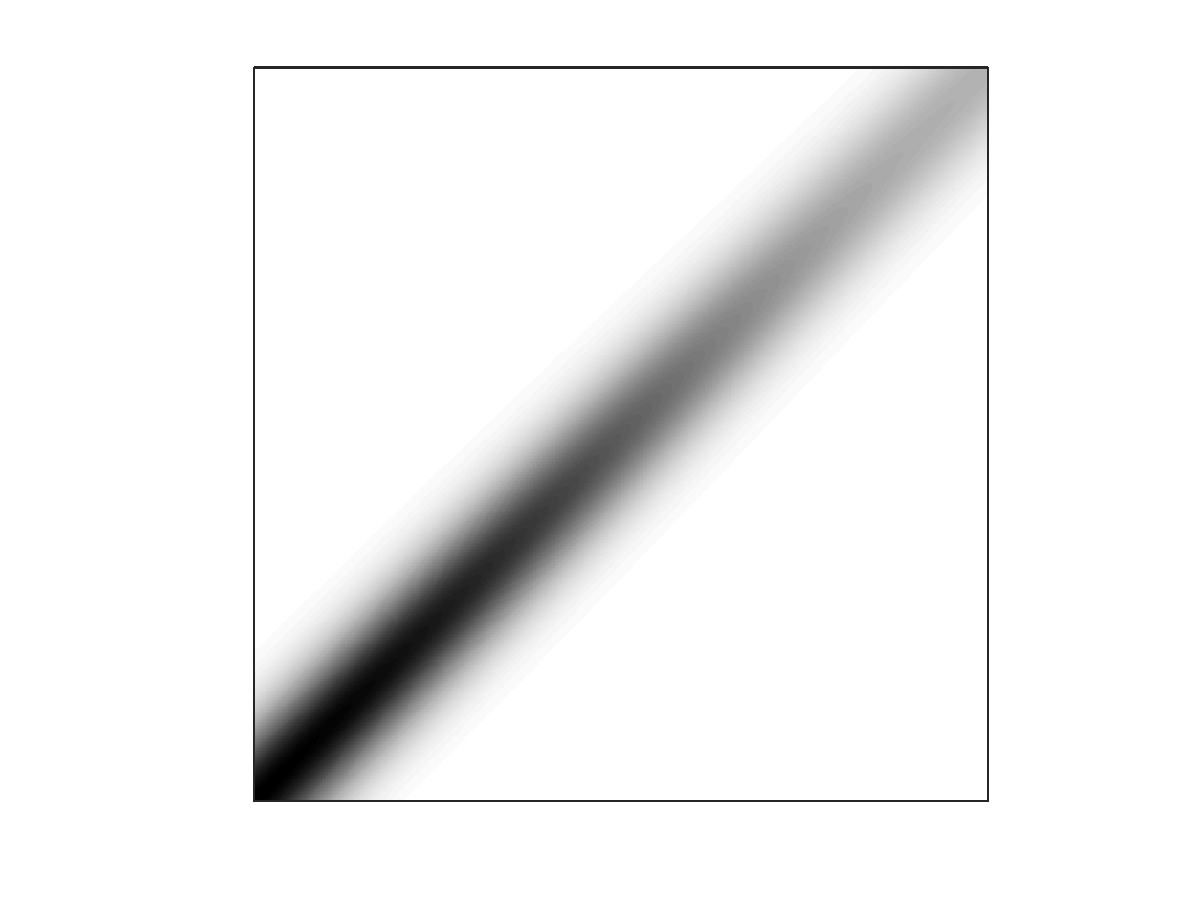 Figure 1
 Figure 2
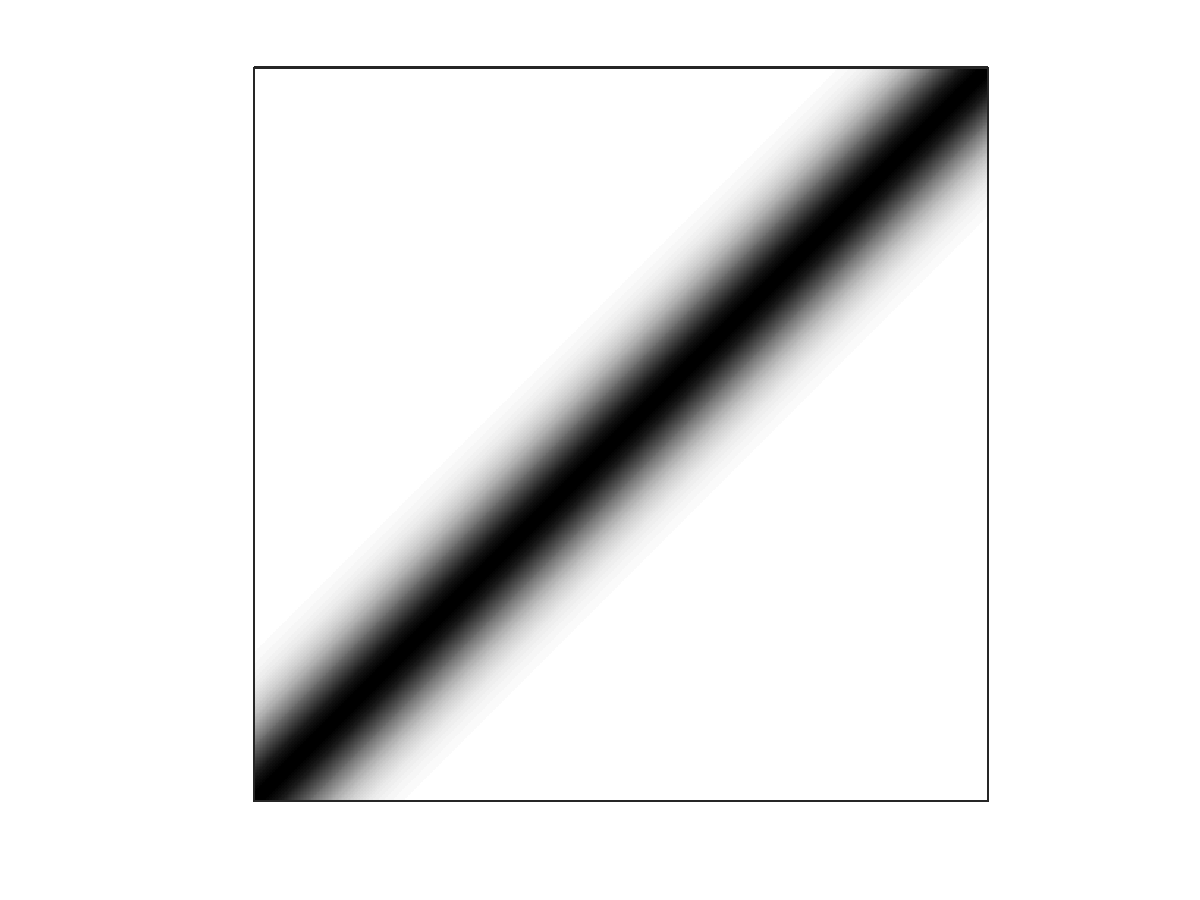 Figure 3
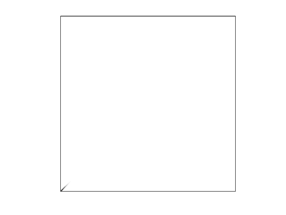 Figure 4
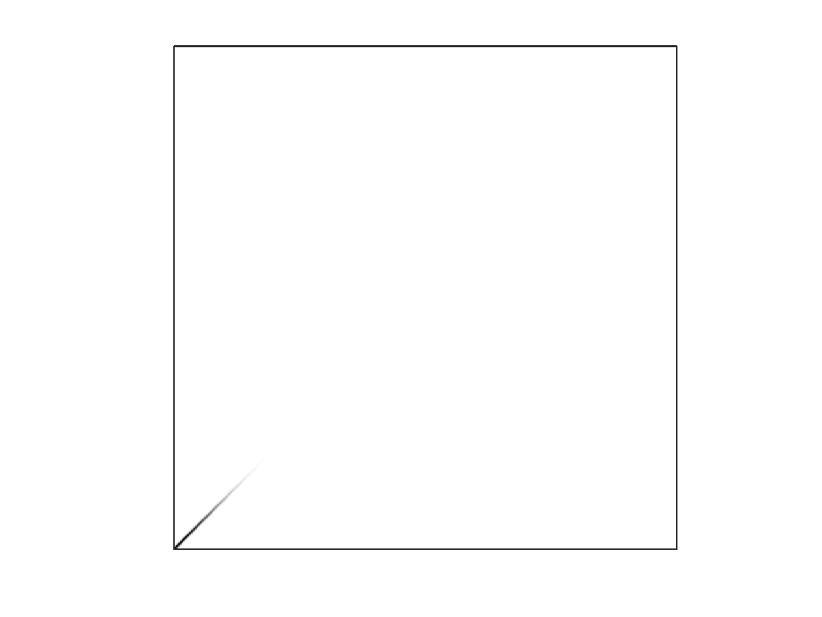 Figure 5
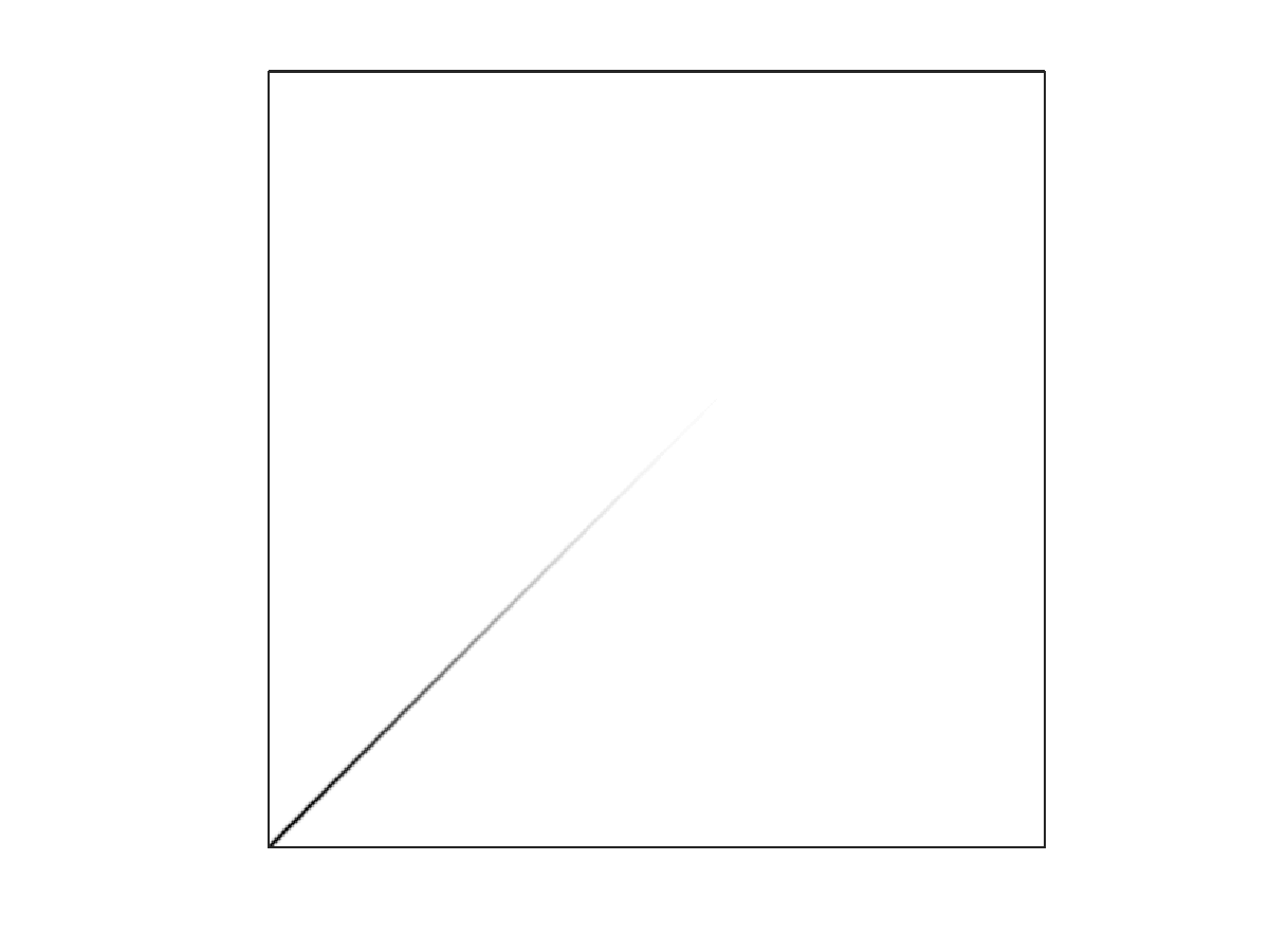 Figure 6
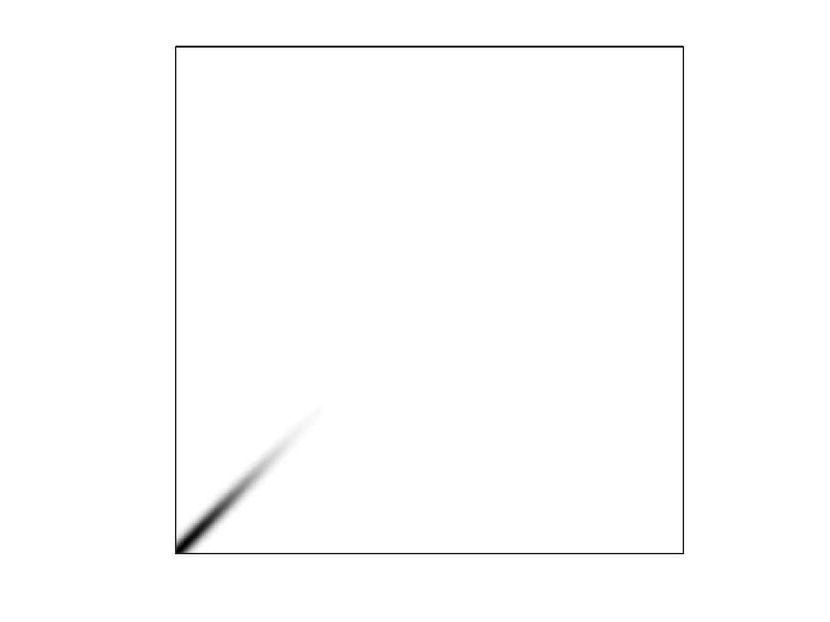 Figure 7
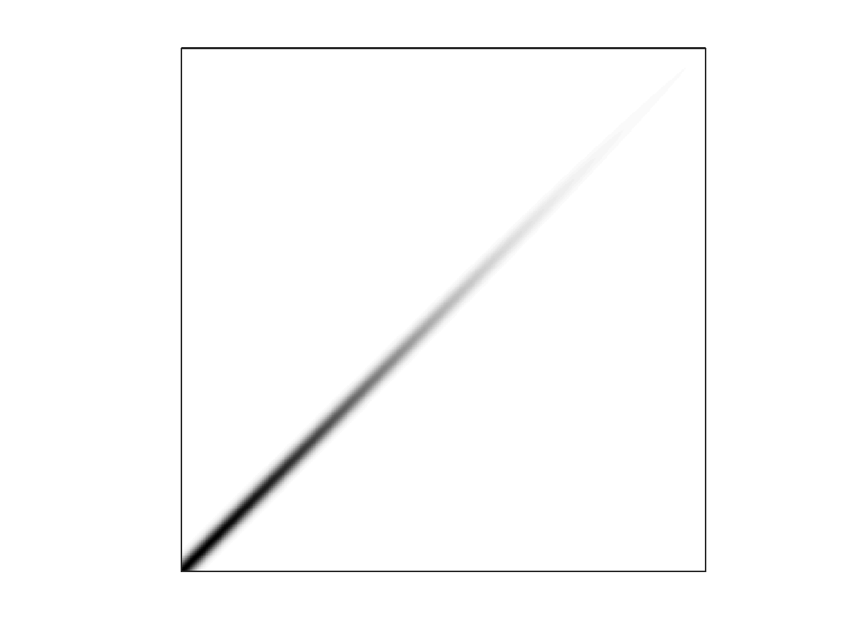 Figure 8
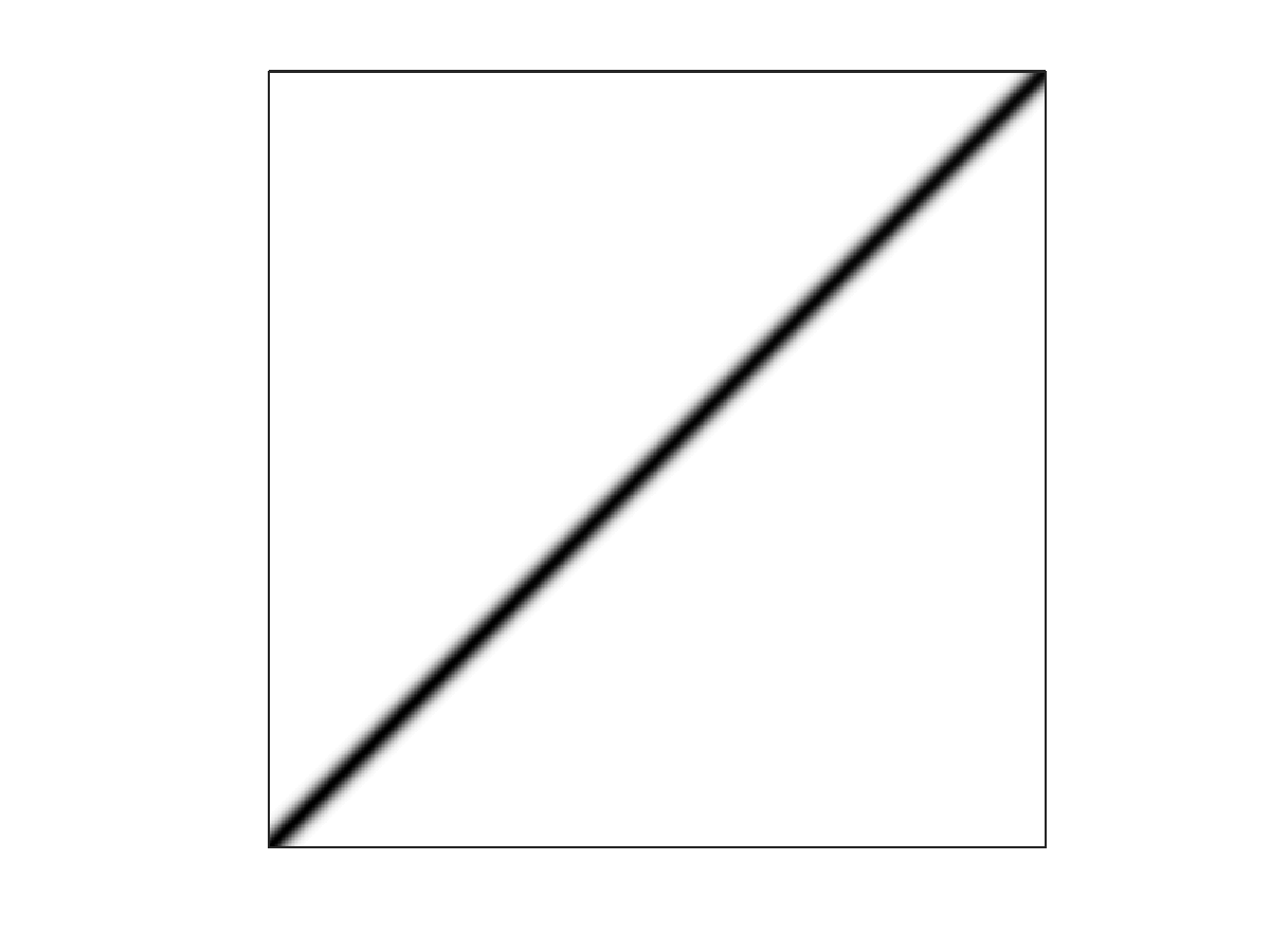 Figure 9
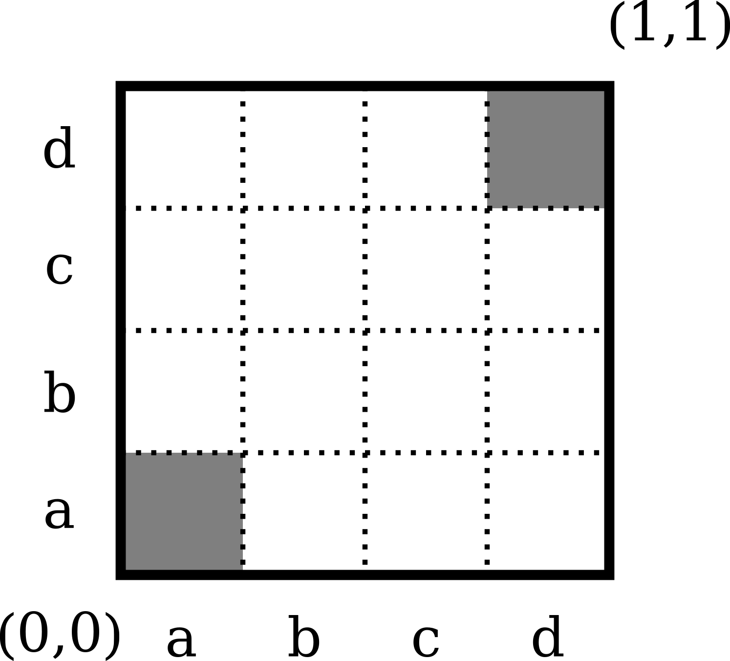 Figure 10
Peer Reviews
No public reviews on file for this paper yet. If you reviewed it on a platform where reviews are public (OpenReview, ICLR, NeurIPS, ICML), you can paste yours below so the community can read it here.
Videos
No videos yet. Explain this paper in a talk, walkthrough, or lecture? Add one.
Taxonomy
TopicsMarkov Chains and Monte Carlo Methods · Stochastic processes and statistical mechanics · Bayesian Methods and Mixture Models
Mixing time of an unaligned Gibbs sampler on the square
Balázs Gerencsér B. Gerencsér is with the Alfréd Rényi Institute of Mathematics, Hungarian Academy of Sciences and the ELTE Eötvös Loránd University, Department of Probability Theory and Statistics, [email protected]. His work is supported by NKFIH (National Research, Development and Innovation Office) grant PD 121107.
Abstract
The paper concerns a particular example of the Gibbs sampler and its mixing efficiency. Coordinates of a point are rerandomized in the unit square to approach a stationary distribution with density proportional to for with some large parameter .
Diaconis conjectured the mixing time of this process to be which we confirm in this paper. This improves on the currently known estimate.
1 Introduction
A standard use of Markov chains is to sample from a probability distribution that would be otherwise hard to access. This can happen when the distribution is supported on a set implicitly defined by some constraints, e.g., a convex body in a high dimensional space [5], [7], proper colorings of a graph [3], [8], etc. Several frameworks have been designed to achieve this goal including the Metropolis algorithm and the Gibbs sampler and their variants. There is a vast range of applications and studies, we refer the reader to [2], [1] for orientation.
A central and recurring question is the efficiency of these algorithms in the different settings. We highlight two phenomena that can decrease the performance of such algorithms. First, the incremental change the Markov chain allows is usually quite rigid and given by the structure of the state space. However, the desired stationary distribution does not need to be aligned with the directions where the Markov chain mixes fast. Second, some boundary effects might occur if the Markov chain can get trapped in some remote part of the state space.
In this paper we analyze an example of the Gibbs sampling procedure proposed by Diaconis which is surprisingly simple considering it captures both of the two phenomena above. We call the coordinate Gibbs sampler for the diagonal distribution the following process. Fix a large positive constant and on define the distribution with density proportional to for . At each step randomly choose coordinate or and rerandomize it according to the conditional distribution of . Notice that the distribution of this Markov chain is mostly concentrated near the diagonal of the unit square, while only horizontal and vertical transitions are allowed. Furthermore, near and we see that both the high density of and also the boundaries of the square hinder the movement of the chain.
The efficiency of the algorithm is quantified by the mixing time of the Markov chain. For any Markov chain on some state space (which is in our case) let denote the distribution of the state at time and be the stationary distribution assuming it is unique (denoted by for our case). Using the total variation distance between measures, we define the mixing time as
[TABLE]
Diaconis conjectured that the mixing time of the example proposed is , the goal of this paper is to confirm this bound.
Theorem 1**.**
Let follow the coordinate Gibbs sampler for the diagonal distribution. For any there exists such that for large enough ,
[TABLE]
Up until now only was known which easily follows from a minorization condition of the transition kernel.
Observe that the diagonal nature of the distribution plays an important role in the mixing behavior, making the distribution and the randomization steps unaligned. If we took the distribution with density proportional to for , then the mixing time would decrease to be . Indeed, this is a product distribution, product of one for and one (uniform) for , consequently after a rerandomization is performed along both coordinates, the distribution of the process will exactly match the prescribed one. This will happen with probability arbitrarily close to 1 within a corresponding finite number of steps, not depending on the value of .
The rest of the paper is organized as follows. In Section 2 a formal definition of the process of interest is provided and further variants are introduced that help the analysis. Section 3 provides the building blocks for the proof, to understand the short-term behavior of the process based on the initialization. Afterwards, the proof of Theorem 1 is aggregated in Section 4. Finally, a complementing lower bound demonstrating that Theorem 1 is essentially sharp is given in Section 5 together with some numerical simulations.
2 Preliminaries, alternative processes
We now formally define the coordinate Gibbs sampler for the diagonal distribution which we denote by , then we introduce variants that will be more convenient to handle.
Let for some large and let be the probability distribution on with density at (where ). We write for the conditional distribution of the coordinate when is fixed (similarly for ). Denote by the projection of , that is, the overall distribution of the coordinate.
When defining the coordinate Gibbs sampler for the diagonal distribution, we separate the decision of the direction of randomization and the randomization itself. For let be an i.i.d. sequence of variables of characters taking both with probability . Given some initial point the random variable is generated as a Markov chain from by randomizing along the axis given by . Formally,
[TABLE]
where are conditionally independent of the past at all steps.
Note that when multiple ’s follow each other in the series (similarly for ), the values are repeatedly overwritten and forgotten, with no further mixing happening for the overall distribution. Therefore we define an alternative process where this effect does not occur, but rather the directions of randomization are deterministic.
Let , then the following process is generated:
[TABLE]
It would be convenient for the analysis if it wasn’t necessary to distinguish the steps based on the parity of the time index. For that reason, consider the following modification. At every even step take as before, at every odd step take flipped along the diagonal of the square (exchange the two coordinates). Equivalently, flip the process at every step while generating. As a result, the randomization happens in the same direction at every step. Note that the target distribution is symmetric along the diagonal therefore no adjustment is needed for the flipping. Formally, the process described is the following:
Let , then the random variables are generated from as follows
[TABLE]
Observe that the scalar process is a Markov chain by itself simply because depends on only through .
3 Dynamics of
In this section we prove two properties of the evolution of , which will be the key elements to compute the mixing time bounds. First, we show that the process cannot stay arbitrarily long at the sides of the unit interval, in or , where some small enough parameter will be chosen. Second, we prove that starting from a point in the middle part , the distribution of the process quickly approaches the stationary distribution.
3.1 Reaching the middle
We work on the case when the is away from the middle of . We want to ensure that the process does not stay near the boundaries for a long period. To quantify this, the time to reach the middle is defined as follows:
Definition 2**.**
Let .
Without the loss of generality we may assume that is on the left part of , thanks to the symmetry of w.r.t. . Therefore we start from . For this period before reaching the middle we introduce a slightly simplified process , where both coordinates are allowed to take values in in principle. This is not supposed to have a substantially different behavior, but will allow more convenient analytic investigation as fewer boundaries are present.
For any let be the measure on with density proportional to conditioned on . Let , then define the Markov chain as follows:
[TABLE]
We can generate to be coupled to as long as possible. For a fixed , is proportional to conditioned on . Therefore, when we need to generate we draw a random sample from and use it for both and if . Otherwise, we use it for but for we draw a new independent sample from . It is easy to verify this is overall a valid method for generating a random variable of distribution .
In the latter case, we also signal decoupling by setting a stopping time . We show this rarely happens, when governed by a variant of . Let .
Lemma 3**.**
For any there is such that .
Proof.
We want to bound the probability of decoupling at every point in time.
When is drawn, is ensured as has not yet occurred. For any we have
[TABLE]
Here we use that the conditional probability is at most twice the unconditional one (because of ), use the monotonicity in , then apply a standard tail probability estimate for the Gaussian distribution.
These exceptional events may occur at most at different times, therefore by using the union bound the overall probability is for any . ∎
Lemma 4**.**
There exists constant such that .
Proof.
By a similar argument as above this bad event happens when but when occurs, then a Gaussian tail probability estimate gives an upper bound of
[TABLE]
The lemma holds with . ∎
Handling is still challenging due to the conditional distributions included in the definition. Therefore we introduce the following process that will be both convenient to handle and to relate to .
Let be a random walk with i.i.d. increments, starting from .
Let .
Let us denote by the distribution of the centered Gaussian with variance . During the analysis of we will also need to use the distribution of the absolute value of a Gaussian distribution with variance . We denote it by when the original one is centered at and it is easy to verify that we can express it for any by .
Proposition 5**.**
* and can be coupled such that for all .*
Proof.
At 0 we have . We construct the coupling iteratively, assuming we perform the next step of the coupling which will satisfy .
We will use the monotone coupling between the two. For two probability distributions the monotone coupling is the one assigning to when . (We now skip currently irrelevant technical details about continuity, etc.). It is easy to verify that is maintained through this coupling exactly if for all . In our case we will need the following:
Lemma 6**.**
For any and :
[TABLE]
Here corresponds to and to and we compare the distributions for step .
Proof.
We are going to prove the following two inequalities:
[TABLE]
For the first of the two we compute :
[TABLE]
[TABLE]
[TABLE]
This last inequality holds because and is decreasing in . Consequently, when is increased to , the measure of decreases confirming the first inequality. This intuitively means that when a Gaussian distribution is shifted to the right then even the reflected Gaussian is shifted (if it was centered at a non-negative point).
The second inequality to confirm is the following:
[TABLE]
We rearrange and cancel out as much as possible from the domain of integrations.
[TABLE]
We substitute the functions to integrate and transform them to compare them on the same domain.
[TABLE]
On all the domain of integration we have . Therefore the exponent is larger at every point for the left hand side, which confirms the second inequality, completing the proof of the lemma. ∎
Lemma 6 thus ensures that the monotone coupling preserves the ordering, and we can indeed use the recursive coupling scheme while keeping at every step. ∎
Proposition 7**.**
For any there exists with the following. For large enough with probability at least we have .
Proof.
First we look at the hitting time analogous to for defined as . Without aiming for tight estimates can be ensured by and by Proposition 5 this holds whenever . The latter is equivalent to .
For some , the distribution of is . Choosing large enough, the probability of this falling into can be made below and this event is a superset of .
Now apply Lemma 3 with . Note that can only happen if . Also Lemma 4 ensures that and almost always coincide. Altogether, we have with an exceptional probability at most , this stays below when is large enough, which completes the proof. ∎
3.2 Diffusion from the middle
In the previous subsection we have seen that the process eventually has to reach the middle of the interval as formulated in Proposition 7. Now we complement the analysis and consider the case when the process is initialized from the middle, meaning . Intuitively, we expect the process to evolve as a random walk with independent Gaussian increments. However, we have to be careful as boundary effects might alter the behavior of when it moves near the ends of the interval . In this subsection we provide the techniques to estimate these boundary effects which will allow to conclude that the mixing of a random walk still translates to comparable mixing of .
Let be a random walk with i.i.d. increments, starting from . Our goal is to couple with which only has a chance as long as stays within .
Definition 8**.**
Let .
Lemma 9**.**
There exist a coupling of the processes and such that whenever .
Proof.
Assume the coupling holds until , having . Let be independent from the past, then define . For , accept if it is in otherwise redraw it according to .
The same values are obtained for the two processes at except if is outside . This is exactly the event we wanted to indicate with when we allow the two processes to decouple. ∎
Lemma 10**.**
For any there exists with the following property. For large enough, if there holds . We also have as we choose .
Proof.
We need to control the minimum and the maximum of a random walk where we use the following result of Erdős and Kac [4]:
Theorem 11** (Erdős-Kac).**
Let i.i.d. random variables, . Let Then for any
[TABLE]
Translating to the current situation, now that we use an initial value as a reference, we want an upper bound on the probability that the partial sums generating never exceed (nor they go below ). The increments have variance and the number of steps is . Formally,
[TABLE]
Now can only occur if this event fails and the maximum exceeds , meaning might exceed 1, or alternatively, the minimum of the process goes below corresponding to possibly leaving at 0. Consequently, we may fix any small , then for any large enough we get
[TABLE]
Observe that the right hand side of the expression indeed converges to 0 as . ∎
Proposition 12**.**
There exists a constant such that for large enough, if we have
[TABLE]
Proof.
We introduce as a parameter. We will find sufficient conditions that ensure the claim of the proposition to hold, then pick a that satisfies the conditions found.
We first compare two simpler distributions, that of and the uniform . By the definition of , the distribution of is .
[TABLE]
The integrand has the form which we replace by (knowing these variables are non-negative). Also, as the probability density functions integrate to 1, we get
[TABLE]
The last inequality follows because the constant term is increased by , so is the length of the domain of the integration but the integrand is bounded above by 1. This step also involves an implicit change of variable depending on , and it results in a final expression independent of this starting condition. The we get is also independent of , it does depend on but has a limit as .
The claim of the lemma is about two other distributions, now we relate them to the ones just compared. Using Lemma 10 for we know that and can be coupled well up to , which directly implies
[TABLE]
where is the constant given by Lemma 10.
To compare with we show converges to in total variation as . For every define
[TABLE]
this is a function proportional to the density of . By standard Gaussian tail estimates for all we get
[TABLE]
Hence for all as . These are uniformly bounded functions, so . The expression to consider for the convergence of the distributions is
[TABLE]
Here is converging to 1 and is therefore bounded after some threshold, so the functions are eventually uniformly bounded and pointwise converging to 0. Thus the integrals also converge, and we get
[TABLE]
We can now combine our bounds of (2), (3) and (4):
[TABLE]
where can be as small as wanted by setting large enough. The proposition holds if we can ensure this sum to be small enough.
Note that a strong compromise is present for the choice of the constant . In (3) we want to limit how likely the boundaries of the unit interval are to be reached, at the same time in (2) we want to show that is already spread out to some extent.
Still, a specific choice is possible. For Lemma 10 provides when using and computer calculations for (1). By choosing but small enough, trusting computers but not too much, we can safely say . In (2) using the same choice of we numerically get for . Once again we allow a safety margin to only claim . ∎
4 Overall mixing
We are now ready to establish mixing time bounds for the process we understand the best, , then we will translate those results to the original process of interest .
Let us define
[TABLE]
which measures the distance from the stationary distribution from the worst starting point. We can give good bounds based on the previous sections:
Lemma 13**.**
There exists a constant such that .
Proof.
Intuitively, from any starting point we can first wait for the process to reach the middle and then let the diffusion happen from there, as these are components we can already control.
Let us apply Proposition 7 with providing a certain . Once the process is in the middle part we know by Proposition 12 that in the subsequent steps sufficient diffusion occurs. Let .
Formally, fix . We perform our calculations by conditioning on the value of .
[TABLE]
Conditioned on , , therefore Proposition 12 provides . We use this for , then performing more steps can only decrease this distance, see [6, Chapter 4] for a detailed discussion about this. For we use the trivial bound on the total variation distance. We get
[TABLE]
∎
A slight variation of compares the distribution of the process when launched from two different starting points.
[TABLE]
Standard results provide the inequalities and the submultiplicativity , see [6, Chapter 4]. The results therein are given for finite state Markov chains but are straightforward to translate to the current case of absolutely continuous distributions and transition kernels.
Proposition 14**.**
For any there exists such that
[TABLE]
Proof.
Using Lemma 13 for any we get
[TABLE]
For this is less than thus by setting the process will be close enough to the stationary distribution as required at . ∎
Lemma 15**.**
The mixing time of and are nearly the same, for any
[TABLE]
Proof.
First, we use that the total variation distance between the marginals is at most the distance between the overall distributions. Consequently, for any we have . This gives .
For the other direction, assume for some . This means there is an optimal coupling with a random variable having distribution such that . As has distribution , it is possible to draw an additional random variable to get with distribution .
This is the same step when generating from thus we may keep the above coupling whenever already present. Therefore we have P\big{(}(Y_{u}(t+1),Y_{u}(t))\neq(\tilde{Y}_{u}^{2},\tilde{Y}_{u}^{1})\big{)}\leq\alpha_{7} which can also be written as . This implies , completing the proof. ∎
We are now ready to prove the main theorem of the paper, as stated in the introduction.
Theorem 1.
Let be the coordinate Gibbs sampler for the diagonal distribution. For any there exists such that for large enough
[TABLE]
Proof.
We use Proposition 14 with and get a constant such that and by Lemma 15 also . At each step the distribution of and might differ only by flipping along the diagonal, which does not change the distance from the (symmetric) thus also leaves the mixing time the same so we get .
The definition of was based on the observation that when the same coordinate is rerandomized repeatedly, no additional mixing happens and the values at that coordinate simply get overwritten. Let us now quantify this effect, counting how many times did the direction of randomization change:
[TABLE]
With this notation we see that for all .
Without the loss of generality we now focus on the case of . Let us express the distribution of conditioning on the value of .
[TABLE]
We substitute and evaluate the total variation distance from .
[TABLE]
The last line holds with some positive by Hoeffding’s inequality for the Binomial distribution and by substituting the upper bound on the total variation distance when we know is above the mixing time. For large enough this is below .
By symmetry, the same bound holds for and by convexity it is also true for the mixture of the two, the unconditional distribution of . This concludes the proof with . ∎
Finally, let us comment on the multitude of constants appearing throughout the proofs, verifying that they can be consistently chosen when needed. First, a small enough has to be picked for the proof of Proposition 12 which also relies on Lemma 10. Once it is fixed, observe that in the remaining Sections 3.1 and 4 all the constants only depend on other ones with lower indices, with the last of Theorem 1 also depending on some previous ones. This excludes the issue of circular dependence.
5 Further estimates
In this section we complement the main result Theorem 1 by a lower bound showing that the order of is exact and by demonstrating the evolution of the distribution via numerical simulations.
Such a lower bound is plausible once having Lemma 9 and Lemma 10, these roughly say that when starting from the middle behaves like a random walk for order of steps and reaches only constant distance in order of steps. Let us proceed by forming a formal argument.
Theorem 16**.**
Let be the coordinate Gibbs sampler for the diagonal distribution. There exists constants such that for large enough
[TABLE]
First of all, to bound the mixing time from below it is sufficient to give a lower bound on the number of steps needed for a single starting point. In this spirit, we set . With this choice, the arguments in Section 3.2 can be applied.
Set . Once we prove for a proper choice of that warrants a large total variation distance at the time and confirms our bound for the mixing time.
Lemma 17**.**
**
Proof.
If we divide the unit square to 4-by-4 equal size smaller squares, then is composed of two of these smaller squares, see Figure 1.
It is enough to show that the selected squares forming have greater or equal probability than the other squares w.r.t. , this directly confirms .
To verify this, we compare the unnormalized density on them. We use the simple inequality that for and any we have
[TABLE]
Indeed, note that is monotone decreasing with . Then for an easy comparison of the arguments provides the bound, while the other cases follow similarly. Observe that for this inequality compares at some point and its reflection to the line . Setting corresponds to a further shift increasing the coordinate after the reflection.
Using this we see that the points of the small square labeled by in Figure 1 correspond to the points of after a reflection so is pointwise larger on by the above inequality. The same comparison holds against where an additional shift is necessary besides the reflection. Consequently, is maximal for the square compared to the others in its column.
Additionally, note that is invariant under the shift of in the direction . Therefore is exactly the same for the four squares on the diagonal. Furthermore, all the other squares are diagonally shifted and/or reflected (w.r.t. the diagonal) copies of the ones considered above, where we have seen that their probability is upper bounded by the probability of the square . The distribution is symmetric w.r.t. the diagonal, so we conclude that (and therefore also ) have indeed maximal probability among all squares. ∎
Lemma 18**.**
For any there exists such that for large enough any satisfies
[TABLE]
Proof.
We want to rely on the previous observations that behaves like a random walk for a while with certain Gaussian increments. Using Lemma 10 we can choose so that the corresponding goes below . Let us denote this by for convenience.
Also, there exists so that
[TABLE]
and clearly the same probability bound holds if the variance is decreased. Fixing , the distribution of is exactly .
To join our estimates we form
[TABLE]
For the first term is below as it is an upper bound for the decoupling of to happen. For the second term is below . Altogether, if ,
[TABLE]
Therefore by choosing we complete the proof. ∎
Proof of Theorem 16.
Apply Lemma 18 with to get some . The distribution of is a mixture of the distributions of and their diagonally flipped version for , where corresponds to how many times the rerandomization happened in a new direction. The set is symmetric w.r.t. the diagonal so for we can simply say it is a convex combination of without needing any correction for the diagonal flip. Now by Lemma 18 each of these probabilities are below , therefore it follows that
[TABLE]
Comparing this with the statement of Lemma 17 we get
[TABLE]
Consequently , so . Thus the theorem holds with the choice . ∎
Finally, we present numerical approximations of the evolution of the distribution over time for different values of . The unit square is discretized with a resolution of and the distribution is calculated along these points. The starting point is always at the lower left corner. The results are presented in Figure 2 for different and different . Both the convergence to the stationary distribution is visible and also how this distribution becomes more concentrated along the diagonal for higher values of . We also computed the time necessary to get within a total variation distance of of the stationary distribution, for , for , for is needed. This is a good proxy for the mixing time, note that only a single (but intuitively bad) starting point was tested and the discretization might have introduced some error. Still, the quadratic growth of with respect to the increase of is already apparent.
Acknowledgments
The author would like to express his thanks to Persi Diaconis and György Michaletzky for their inspiring comments and to the American Institute of Mathematics for the stimulating workshop they hosted and organized.
The reference list from the paper itself. Each links out to its DOI / PubMed record.
- 1[1] P. Diaconis , The Markov chain Monte Carlo revolution , Bulletin of the American Mathematical Society, 46 (2009), pp. 179–205.
- 2[2] P. Diaconis and L. Saloff-Coste , What do we know about the Metropolis algorithm? , Journal of Computer and System Sciences, 57 (1998), pp. 20–36.
- 3[3] M. Dyer, A. D. Flaxman, A. M. Frieze, and E. Vigoda , Randomly coloring sparse random graphs with fewer colors than the maximum degree , Random Structures & Algorithms, 29 (2006), pp. 450–465.
- 4[4] P. Erdős and M. Kac , On certain limit theorems of the theory of probability , Bulletin of the American Mathematical Society, 52 (1946), pp. 292–302.
- 5[5] R. Kannan, L. Lovász, and M. Simonovits , Random walks and an O ∗ ( n 5 ) superscript 𝑂 superscript 𝑛 5 {O}^{*}(n^{5}) volume algorithm for convex bodies , Random Structures & Algorithms, 11 (1997), pp. 1–50.
- 6[6] D. Levin, Y. Peres, and E. Wilmer , Markov chains and mixing times , American Mathematical Society, 2009.
- 7[7] L. Lovász and S. Vempala , Simulated annealing in convex bodies and an O ∗ ( n 4 ) superscript 𝑂 superscript 𝑛 4 {O^{*}}(n^{4}) volume algorithm , Journal of Computer and System Sciences, 72 (2006), pp. 392–417.
- 8[8] E. Mossel and A. Sly , Gibbs rapidly samples colorings of G ( n , d / n ) 𝐺 𝑛 𝑑 𝑛 {G}(n,d/n) , Probability Theory and Related Fields, 148 (2010), pp. 37–69.