Forbidden branches in trees with minimal atom-bond connectivity index
Darko Dimitrov, Zhibin Du, Carlos M. da Fonseca

TL;DR
This paper investigates the structural properties of trees with the minimal atom-bond connectivity (ABC) index, revealing restrictions on certain branch configurations to advance their complete characterization in chemical graph theory.
Contribution
It establishes new structural constraints on minimal-ABC trees, specifically ruling out the coexistence of certain branch types, thus progressing toward their full classification.
Findings
Minimal-ABC trees cannot contain both a B4-branch and B1 or B2-branches simultaneously.
Provides new structural properties that limit the configurations of minimal-ABC trees.
Advances understanding of the structure of trees with minimal atom-bond connectivity index.
Abstract
The atom-bond connectivity (ABC) index has been, in recent years, one of the most actively studied vertex-degree-based graph invariants in chemical graph theory. For a given graph , the ABC index is defined as , where is the degree of vertex in and denotes the set of edges of . In this paper we present some new structural properties of trees with a minimal ABC index (also refer to as a minimal-ABC tree), which is a step further towards understanding their complete characterization. We show that a minimal-ABC tree cannot simultaneously contain a -branch and or -branches.
Click any figure to enlarge with its caption.
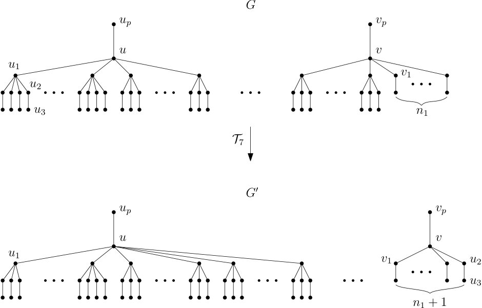 Figure 1
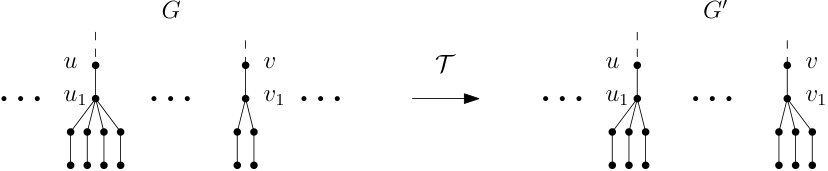 Figure 2
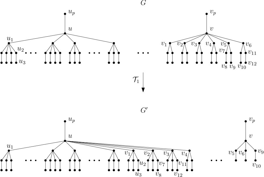 Figure 3
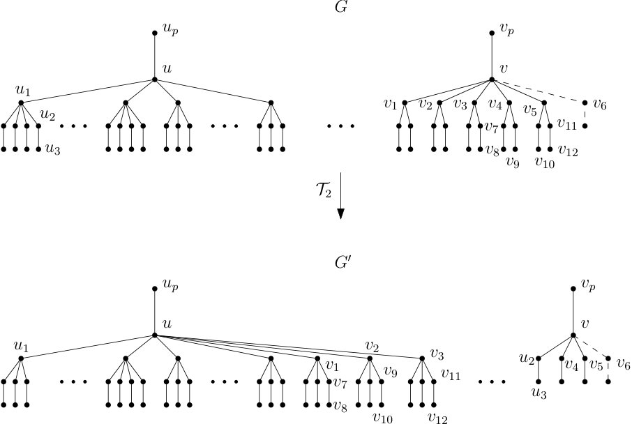 Figure 4
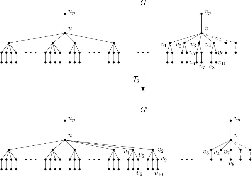 Figure 5
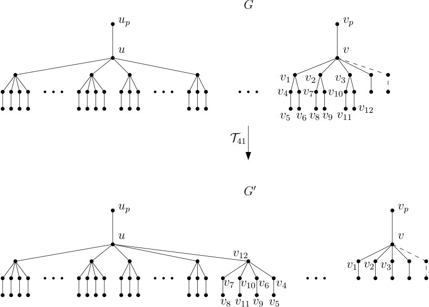 Figure 6
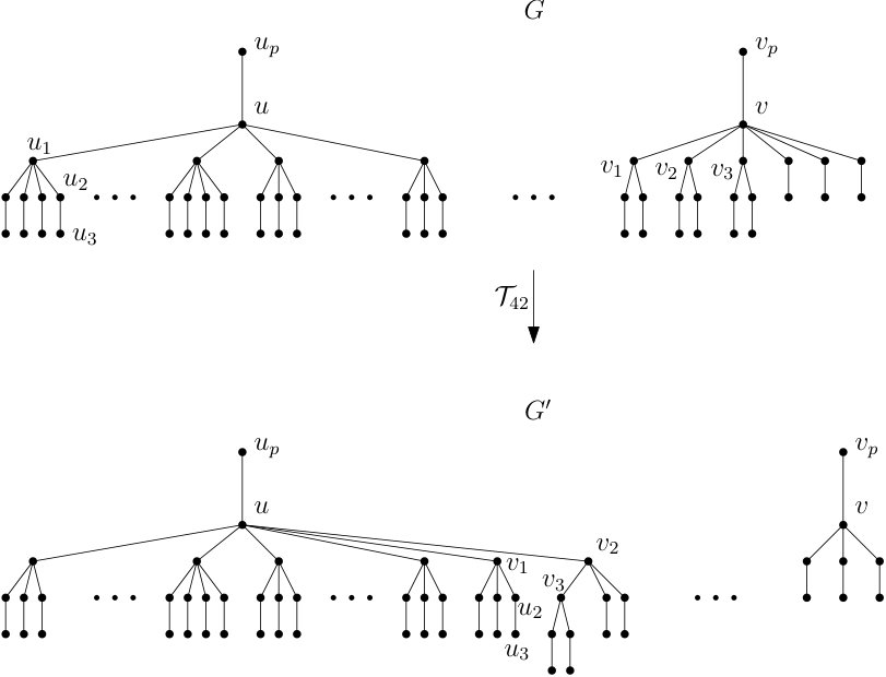 Figure 7
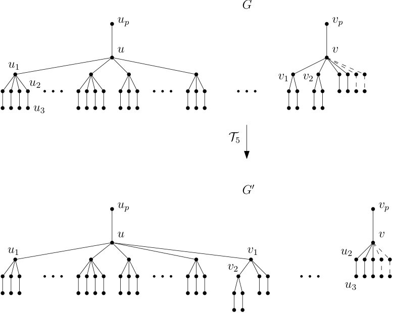 Figure 8
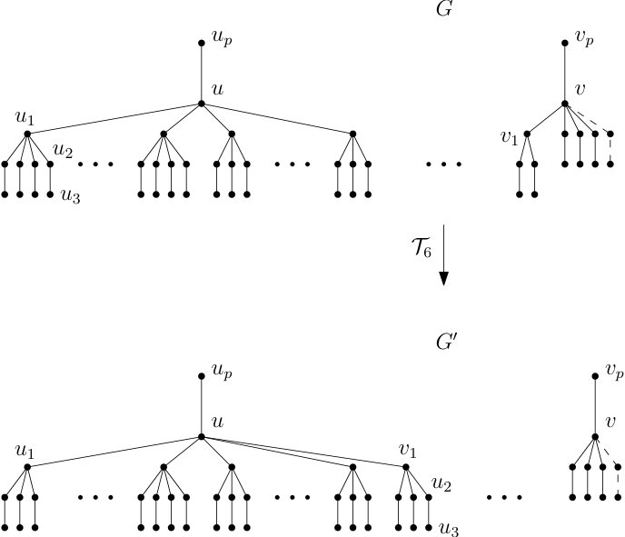 Figure 9
Peer Reviews
No public reviews on file for this paper yet. If you reviewed it on a platform where reviews are public (OpenReview, ICLR, NeurIPS, ICML), you can paste yours below so the community can read it here.
Videos
No videos yet. Explain this paper in a talk, walkthrough, or lecture? Add one.
Forbidden branches in trees
with minimal atom-bond connectivity index
Abstract
The atom-bond connectivity (ABC) index has been, in recent years, one of the most actively studied vertex-degree-based graph invariants in chemical graph theory. For a given graph , the ABC index is defined as , where is the degree of vertex in and denotes the set of edges of . In this paper we present some new structural properties of trees with a minimal ABC index (also refer to as a minimal-ABC tree), which is a step further towards understanding their complete characterization. We show that a minimal-ABC tree cannot simultaneously contain a -branch and or -branches.
Darko Dimitrova, Zhibin Dub, Carlos M. da Fonsecac,d
*a**Hochschule für Technik und Wirtschaft Berlin, Germany &
Faculty of Information Studies, Novo Mesto, Slovenia*
E-mail: [email protected]
*b**School of Mathematics and Statistics, Zhaoqing University
Zhaoqing 526061, China*
E-mail: [email protected]
*c**Department of Mathematics, Kuwait University
Safat 13060, Kuwait*
E-mail: [email protected]
*d**Department of Mathematics, University of Primorska
Glagoljsaška 8, 6000 Koper, Slovenia*
E-mail: [email protected]
Keywords: Atom-bond connectivity index; tree; extremal graphs
1 Introduction and preliminaries
Let be a simple undirected graph with vertices. For , the degree of , denoted by , is the number of edges incident to . In 1998, Estrada, Torres, Rodríguez and Gutman [21] proposed a vertex-degree-based graph topological index - the atom-bond connectivity (ABC) index - defined as
[TABLE]
where
[TABLE]
It was shown that the ABC index can be a valuable predictive tool in the study of heat formation in alkanes. Ten years later, Estrada elaborated in [20] an innovative quantum-theory-like explanation of this topological index. Incontestably, this topic has triggered tremendous interest in both mathematical and chemical research communities, leading to a number of results that incorporate the structural properties and the computational aspects of the graphs with extremal properties [1, 2, 3, 4, 5, 10, 7, 14, 15, 16, 17, 8, 9, 18, 23, 29, 25, 27, 22, 31, 30, 36, 38, 40, 42, 43, 44, 46, 24, 11, 35, 39]. On the other hand, the physico-chemical applicability of the ABC index has also been confirmed and extended in several other studies [6, 28, 32, 34, 45].
It has been proven that deleting/adding an edge in a graph strictly decreases/increases its ABC index [4, 8]. Consequently, among all connected graphs, a tree/the complete graph has minimal/maximal ABC index.
It has been shown that among the trees of a given order, the star is the one with maximal ABC index [23]. Notwithstanding, a thoroughgoing characterization of trees with minimal ABC index, also referred to as minimal-ABC trees, still remains an open problem. This paper represents a step further towards the comprehensive classification of such trees.
In the sequel, we present some additional results and main notations that will be used throughout the paper. A vertex of degree one is a pendant vertex. As in [31], a sequence of vertices of a graph , , will be called a pendant path if each two consecutive vertices in are adjacent in , , , for , and . The length of the pendant path is . If , then is called an internal path of length .
A -branch is a path of length attached to a vertex that has at least one child of degree at least 3. We call the vertex of degree in a -branch as the center of such -branch. A -branch, for , is a (sub)graph comprised of vertex of degree and pendant paths of length that all have as a common vertex. We call the vertex also the center of the -branch. Moreover, a -branch, for , is a (sub)graph obtainable from by attaching an additional vertex to a pendant vertex of -branch.
A -terminal vertex of a rooted tree is a vertex of degree , which is a parent of only -branches, such that at least one branch among them is a -branch (or -branch). The (sub)tree, induced by a -terminal vertex and all its (direct and indirect) children vertices, is called a -terminal branch or -branch.
A sequence is graphical if there is a graph whose vertex degrees are , . Additionally, if , then is called a degree sequence.
To determine the minimal-ABC trees with an order less than is a simple task, therefore to simplify the exposition in the rest of the paper, we assume that all the trees are of an order at least .
In , Wang [41] defined a greedy tree as follows.
Definition 1.1**.**
Suppose the degrees of the non-leaf vertices are given, the greedy tree is achieved by the following ‘greedy algorithm’:
Label the vertex with the largest degree as (the root). 2. 2.
Label the neighbors of as assign the largest degrees available to them such that . 3. 3.
Label the neighbors of (except ) as such that they take all the largest degrees available and that then do the same for . 4. 4.
Continue the labeling of the unlabeled vertices in the same manner as in 3., always starting with the neighbors of the labeled vertex with the largest degree.
Next we present the so-called switching transformation explicitly stated by Lin, Gao, Chen, and Lin [37]. The switching transformation was used in the proofs of some characterizations of the minimal-ABC trees, as it was the case with Lemma 1.2 by Gan, Liu, and You in [26].
Lemma 1.1** (Switching transformation).**
Let be a connected graph with and . Let . If and , then , with the equality if and only if or .
Lemma 1.2**.**
In a minimal-ABC tree, every path , where and are leaves, has the properties:
if is odd, then
[TABLE] 2. 2.
if is even, then
[TABLE]
Almost simultaneously, Xing and Zhou [42], Gan, Liu, and You [26] and Lin, Gao, Chen, and Lin [37] independently gave the following characterization.
Theorem 1.3**.**
Given the degree sequence, the greedy tree minimizes the ABC index.
In [31], Gutman, Furtula, and Ivanović obtained the following result.
Theorem 1.4**.**
A minimal-ABC tree with vertices contains neither internal paths of any length nor pendant paths of length .
An immediate, but important, consequence of Theorem 1.4 is the next corollary [31, 42].
Corollary 1.5**.**
Let be a minimal-ABC tree. Then the subgraph induced by the vertices of whose degrees are greater than two is also a tree.
An improvement of Theorem 1.4 is the following result by Lin, Lin, Gao, and Wu [38].
Theorem 1.6**.**
Each pendant vertex of a minimal-ABC tree belongs to a pendant path of length , where or .
Further improvement of Theorem 1.4 was given by Gutman, Furtula, and Ivanović.
Theorem 1.7** ([31]).**
The -vertex tree, , with minimal ABC-index contains at most one pendant path of length .
By Theorem 1.6 and Corollary 1.5, it follows that the minimal-ABC trees can be obtained by unifying each pendant vertex of a tree with the center vertex of a -branch. In particular, if is just a star, then the minimal-ABC trees are the same trees that are minimal with respect to Kragujevac trees [33].
In [13] it was shown that a minimal-ABC tree contains at most one -branch, . The next three results, which will be used in the proofs in the next two sections, considering the bounds on the number of -branches, a (non)coexistence of some types of -branches that have a common parent vertex as well as some conditions on the existence of pendant path of length .
Theorem 1.8** ([12]).**
A minimal-ABC tree does not contain a -branch, .
Theorem 1.9** ([12]).**
A minimal-ABC tree does not contain more than four -branches.
Theorem 1.10** ([13]).**
A minimal-ABC tree contains at most four -branches. Moreover, if is a -branch itself, then it contains at most three -branches.
Lemma 1.11** ([12]).**
A minimal-ABC tree does not contain
- (a)
a -branch and a -branch, 2. (b)
a -branch and a -branch,
that have a common parent vertex.
Lemma 1.12** ([19]).**
A minimal-ABC tree does not contain a -branch and a -branch that have a common parent vertex.
Theorem 1.13** ([16]).**
A minimal-ABC tree of order with a pendant path of length may contain -branches if and only if it is of order or . Moreover, in this case the minimal-ABC tree is comprised of a single central vertex, -branches and one -branch, including a pendant path of length that may belong to a - or -branch.
For further properties of the minimal-ABC trees, the reader is referred to [11, 12, 13, 16, 18, 19]. Before we proceed with the main results of this paper, we present the following observation that will be applied in the further analysis.
Observation 1.1**.**
*Let be a minimal-ABC tree with the root vertex and let be the sequence of vertices obtain by the breadth-first search of . If and , then by Lemma 1.1, we may assume that . *
In what follows, we will present some new structural properties of minimal-ABC trees by strengthening Lemma 1.11. In Section 2 we will show that a minimal-ABC tree cannot contain a -branch and a -branch simultaneously, while in Section 3 we will show that a minimal-ABC tree cannot contain a -branch and a -branch simultaneously.
2 Trees containing simultaneously - and -branches
This section is devoted to proving that a minimal-ABC tree cannot contain a -branch and a -branch simultaneously. First we state two technical lemmas which will be particularly useful throughout the paper. For the proof the reader can be referred to [12]. The function is defined as in (1).
Lemma 2.1**.**
Let , with real numbers , , . Then increases in and decreases in .
Due to the symmetry of , Lemma 2.1 can be rewritten as follows.
Lemma 2.2**.**
Let , with real numbers , , . Then decreases in and increases in .
First, we present two crucial properties for the minimal-ABC trees, which will be applied in the proof of the main result in this section - Theorem 2.5.
Proposition 2.3**.**
A minimal-ABC tree cannot contain a -branch and a -branch simultaneously, where is the parent vertex of the center of a -branch, and is the parent vertex of the center of a -branch, when
- •
* and ;*
- •
* and ;*
- •
* and .*
Proof.
Suppose that is a minimal-ABC tree that contains a -branch and a -branch simultaneously. Let be the center vertex of a -branch, with the parent vertex , and the center vertex of a -branch, with the parent vertex . From Observation 1.1, we know that occurs before in the breadth-first search of . Furthermore, by Lemma 1.1, it follows that .
Here we apply the transformation depicted in Figure 1.
After applying , the change of the ABC index of is
[TABLE]
By Lemma 2.1, increases in . For , it can be verified that , respectively, are the smallest values of for which is non-negative.
For , we obtain that
[TABLE]
i.e., the function is negative.
By Lemma 2.2, we have that decreases in , and thus also
[TABLE]
for .
Now the result follows. ∎
Applying the inverse transformation of the transformation depicted in Figure 1, together with the proof of Proposition 2.3, the following proposition is immediate.
Proposition 2.4**.**
A minimal-ABC tree cannot contain two -branches, attached to two different vertices, simultaneously, where and are the two (different) parent vertices of the centers of two -branches, when
- •
* and ;*
- •
* and ;*
- •
* and .*
We now state and prove the main result of this section.
Theorem 2.5**.**
A minimal-ABC tree cannot contain a -branch and a -branch simultaneously.
Proof.
Suppose that is a minimal-ABC tree that contains a -branch and a -branch simultaneously. Let be the center vertex of a -branch, with the parent vertex and the grandparent vertex (if existed). Let be the last vertex in the breadth-first search of , which is a parent of a -branch. Denote by the center vertex of that -branch and the parent of . Here also, by Observation 1.1, we have occurs before in the breadth-first search of . Furthermore, by Lemma 1.1, it follows that . Notice that the existence of - and -branches in implies that every pendant path in is of length , from Theorem 1.13.
By Lemma 1.11(b), and cannot have a common parent vertex, i.e., . And by Proposition 2.3, the following cases remain to be considered:
- •
and ;
- •
and ;
- •
and .
By Lemma 1.11(b), cannot be a parent vertex of a -branch. And we will show that cannot be a parent vertex of a -branch, either.
Suppose to the contrary that there is a -branch attached to . From Proposition 2.4, no -branch is attached to .
Suppose that every branch attached to is a -branch, except the one containing (not necessarily exist such branch). By Lemma 1.1 and Lemma 1.11(b), we know that every branch attached to is actually a -branch. However, Theorem 1.9 claims that there are at most four -branches in , which is a contradiction to .
Suppose that there is a branch attached to which is not a -branch, denote by the child of in such branch. If occurs before in the breadth-first search of , then by Observation 1.1, there must have -branch attached to , which is a contradiction to the choice of . If occurs before in the breadth-first search of ( is also a child of ), then by Observation 1.1, either there exists -branch attached to , which is a contradiction to Proposition 2.4, or there are at least five -branch in , which is a contradiction to Theorem 1.9.
So no -branch is attached to , i.e., every branch attached to is - or -branch.
Let and be the number of - and -branches, correspondingly, that have as the parent vertex. It holds that , with and . Moreover, by Theorem 1.10, can be at most .
In the rest of the proof, we will consider the remaining cases when . Further, we distinguish six cases with respect to the value of : .
In addition, notice that cannot occur before in the breadth-first search of , and recalling that from Lemma 1.11(b), thus there are four possibilities with respect to the relationship between vertices and , that we are interested in:
- (a)
and are all different vertices;
- (b)
and denote the same vertex (i.e., );
- (c)
is the parent of (i.e., ), and is not the root vertex of ;
- (d)
is the parent of (i.e., ), and is the root vertex of .
In the analysis of the following cases, first we will consider case (a). With the remaining cases (b), (c) and (d), we will proceed similarly.
Case . .
First we consider case (a), i.e., and are pairwise distinct vertices. Notice that in this case and .
Here we apply the transformation depicted in Figure 2.
After applying , the degree of the vertex increases by , the degrees of the vertices and increase by , the degree of decreases by , while the degrees of , , one child of and one child of decrease by , and the rest of the vertices do not change their degrees.
The change of the ABC index after applying is
[TABLE]
where , for , are the neighbors of in , except .
Clearly,
[TABLE]
for all , and both and decrease in . On the other hand, by Lemmas 2.2 and 2.1, and increase in and , respectively, which implies that
[TABLE]
and
[TABLE]
Now we have
[TABLE]
since , when . Thus, we have shown that the change of the ABC index after applying the transformation is negative, which is a contradiction to the initial assumption that is a minimal-ABC tree.
In the above deduction for case (a), notice that the term on may be neglected, thus, in case (b), i.e., when , we may obtain the same negative upper bound for the change of the ABC index after applying as in (4).
For case (c), i.e., when and is not the root vertex of , we can obtain the same upper bound for the change of the ABC index after applying , just by replacing with in (3), i.e.,
[TABLE]
Furthermore, similar to the argument regarding (4), we can obtain the same negative upper bound for as in (4).
Notice that (5) is independent of that if is the root vertex of (i.e., the existence of the parent of ), thus the upper bounds in cases (c) and (d) are actually the same.
Case . .
First we consider case (a), i.e., and are pairwise distinct vertices. In this case, either (i.e., ) or (i.e., ).
Here, we apply the transformation depicted in Figure 3.
After applying , the degree of the vertex increases by , the degrees of the vertices and increase by , the degree of decreases by , while the degrees of , , one child of and one child of decrease by , and the rest of the vertices do not change their degrees.
The change of the ABC index after applying is
[TABLE]
where , for , are all the neighbors of in , except .
A similar analysis as in Case shows that
[TABLE]
Recall that here or , and then or , respectively. Observe that the right-hand side of (6) decreases in . Thus, for , we obtain the upper bound on (6) when , which is . In the case of , the upper bound on (6) is obtained when and it is .
The proofs for cases (b), (c) and (d) are similar to case (a), and the detailed illustration can be referred to that in Case .
Case . .
First we consider case (a), i.e., and are all different vertices. In this case, and , correspondingly.
Here, we apply the transformation depicted in Figure 4.
After applying , the degree of the vertex increases by , the degrees of the vertices and increase by , the degrees of , one child of and one child of decrease by , and the rest of the vertices do not change their degrees.
The change of the ABC index after applying is
[TABLE]
where , for , are all the neighbors of in .
Similar analysis as in Case shows that
[TABLE]
Clearly, the right-hand side of (8) decreases in , so the negative change of the ABC index follows again from direct calculation, except the cases and . For this case, we need only to analyze the following term in (7):
[TABLE]
Note that, from Lemma 2.2, decreases in , and from Lemmas 1.1 and 1.11(b), the possible minimum degree among all the neighbors of in , different from and , is . Thus
[TABLE]
Now, it follows that
[TABLE]
Subsequently a negative upper bound follows from direct calculation, for and .
The proofs for cases (b), (c) and (d) are similar to that in case (a), and the detailed illustration can be referred to that in Case .
Case . .
First we consider case (a), i.e., and are pairwise distinct vertices. In this case, and , correspondingly. We distinguish two subcases regarding the degree of the vertex .
Subcase . .
Here, we apply the transformation depicted in Figure 5.
After applying , the degrees of the vertices and increase by , the vertex increases its degree from to , while and one child from each decrease their degrees by , the rest of the vertices do not change their degrees.
The change of the ABC index after applying is
[TABLE]
where , for , are all the neighbors of in .
Clearly,
[TABLE]
for all , thus one can obtain that
[TABLE]
Notice that the right-hand side of (10) decreases in , thus the negative change of the ABC index follows, except the cases where
- •
and ;
- •
and .
For the remaining cases, we need only to consider (9), in particular the term
[TABLE]
Note that, from Lemma 2.2, decreases in , and from Lemmas 1.1 and 1.11(b), the possible minimum degree among all the neighbors of in , different from and , is . Hence
[TABLE]
Now, it follows that
[TABLE]
Consequently we get a negative upper bound by direct calculation.
Subcase . .
In this case, the number of the -branches is , i.e., . Here, we apply the transformation depicted in Figure 6.
After applying , the degree of the vertex increases by , the degrees of and increase from to , the degree of after applying is , the degree of decreases from to , and the rest of the vertices do not change their degrees.
The change of the ABC index after applying is
[TABLE]
where , for , are the neighbors of in , except . An analogous analysis to Case shows that
[TABLE]
Clearly, the right-hand side of (12) decreases in , so the negative change of the ABC index follows.
The proofs for cases (b), (c) and (d) are similar to case (a), and the detailed illustration can be referred to that in Case .
Case . .
First we consider case (a). In this case, since , we have that , correspondingly. Here, we apply the transformation depicted in Figure 7.
After applying , the degree of the vertex increases by , the degree of increases from to , the degree of the vertex decreases by , the degree of decreases from to , and the rest of the vertices do not change their degrees.
The change of the ABC index after applying is
[TABLE]
where , for , are the neighbors of in , except . Similar technique in Case shows that
[TABLE]
Clearly, the right-hand side of (14) decreases in , so the fact that the change of the ABC index being negative follows from direct calculation, except the cases where
- •
and ;
- •
and ;
- •
and .
For the above cases, we need only to analyze in (13) the term
[TABLE]
Note that, from Lemma 2.2, decreases in , and from Lemmas 1.1 and 1.11(b), the possible minimum degree among all the neighbors of in , different from and , is . Therefore, we have
[TABLE]
Now, we obtain
[TABLE]
Subsequently a negative upper bound follows from direct calculation.
The proofs for cases (b), (c) and (d) are similar to that in case (a), and the detailed illustration can be referred to that in Case .
Case . .
First we consider case (a), i.e., and are pairwise distinct vertices. By Theorem 1.10 . Thus, there are two possible configurations in this case: and , correspondingly. Here, we apply the transformation depicted in Figure 8.
After applying , the degree of the vertex increases by , the degree of increases from to , the degree of the vertex decreases by , the degree of decreases from to , and the rest of the vertices do not change their degrees.
The change of the ABC index after applying is
[TABLE]
where , for , are the neighbors of in different from . A similar analysis as in Case shows that
[TABLE]
Clearly, the right-hand side of (16) decreases in , so we can get a negative upper bound through direct calculation, except for the case when and .
For the remaining cases, we need only to consider the term (15), which is as follows
[TABLE]
Note that, from Lemma 2.2, decreases in , and from Lemmas 1.1 and 1.11(b), the possible minimum degree among all the neighbors of in , different from and , is , thus
[TABLE]
Now what follows is that
[TABLE]
Subsequently a negative upper bound follows from direct calculation.
The proofs for cases (b), (c) and (d) are similar to that in case (a), and as before the detailed illustration can be referred to that in Case .
By combining the above six cases, the claim of the theorem is finally obtained. ∎
3 Trees containing simultaneously - and -branches
In the final section we prove that a minimal-ABC tree does not contain a -branch and a -branch in simultaneity.
Theorem 3.1**.**
A minimal-ABC tree cannot contain a -branch and a -branch simultaneously.
Proof.
Let be the center vertex of a -branch and the center vertex of a -branch in a minimal-ABC tree . By Lemma 1.11(a), and cannot have a common parent vertex. So, let be the parent of , and the parent of if is not the root vertex of . Similarly, let be the parent of , and the parent of .
On one hand, by Theorem 2.5 and Lemma 1.11(a), neither - nor -branch can be attached to . On the other hand, since has -branches as children, thus has a child of degree at least , i.e., there must exist some -branches attached to , which also implies that no -branch can be attached to from Lemma 1.12. In conclusion, the branches attached to can only be - or -branches. Here also, by Observation 1.1, we may assume that occurs before in the breadth-first search of . Furthermore, by Lemma 1.1, it follows that .
First, we consider case (a), i.e., when the vertices and are pairwise distinct. Denote by the number of -branches attached to in . Let us consider the transformation depicted in Figure 9.
After applying , the degree of increases by , the degree of decreases by , while the degree of decreases by , and the rest of the vertices do not change their degrees.
The change of the ABC index after applying is
[TABLE]
where , for , are all the neighbors of in , with the exception of .
We remark that , since has -branches. Then, as previously, we obtain
[TABLE]
Clearly, the right-hand side of (17) decreases in , so we can obtain a negative upper bound through direct calculation procedure. Finally, the proofs for the remaining cases of (b), (c), and (d) are very similar to this one. ∎
4 Acknowledgment
The authors would like to thank the anonymous reviewers for their insightful comments. The authors are especially indebted to the reviewer whose observations also aided in the shortening the proof of Theorem 2.5.
The reference list from the paper itself. Each links out to its DOI / PubMed record.
- 1[1] M. B. Ahmadi, D. Dimitrov, I. Gutman, S. A. Hosseini, Disproving a conjecture on trees with minimal atom-bond connectivity index , MATCH Commun. Math. Comput. Chem. 72 (2014) 685–698.
- 2[2] M. B. Ahmadi, S. A. Hosseini, P. Salehi Nowbandegani, On trees with minimal atom bond connectivity index , MATCH Commun. Math. Comput. Chem. 69 (2013) 559–563.
- 3[3] M. B. Ahmadi, S. A. Hosseini, M. Zarrinderakht, On large trees with minimal atom–bond connectivity index , MATCH Commun. Math. Comput. Chem. 69 (2013) 565–569.
- 4[4] J. Chen, X. Guo, Extreme atom-bond connectivity index of graphs , MATCH Commun. Math. Comput. Chem. 65 (2011) 713–722.
- 5[5] J. Chen, J. Liu, X. Guo, Some upper bounds for the atom-bond connectivity index of graphs , Appl. Math. Lett. 25 (2012) 1077–1081.
- 6[6] J. Chen, J. Liu, Q. Li, The atom-bond connectivity index of catacondensed polyomino graphs , Discrete Dyn. Nat. Soc. 2013 (2013) ID 598517.
- 7[7] K. C. Das, Atom-bond connectivity index of graphs , Discrete Appl. Math. 158 (2010) 1181–1188.
- 8[8] K. C. Das, I. Gutman, B. Furtula, On atom-bond connectivity index , Chem. Phys. Lett. 511 (2011) 452–454.