Behaviour of the Serre Equations in the Presence of Steep Gradients Revisited
Jordan Pitt, Christopher Zoppou, Stephen Roberts

TL;DR
This study uses numerical methods to analyze the behaviour of the Serre equations with steep gradients, revealing new solution structures and assessing the accuracy of shallow water and asymptotic approximations.
Contribution
It introduces a numerical investigation of the Serre equations with steep initial conditions, identifying new solution structures and evaluating analytical and asymptotic approximations.
Findings
Four solution structures depending on steepness
Two structures align with existing literature
Two novel solution structures identified
Abstract
We use numerical methods to study the behaviour of the Serre equations in the presence of steep gradients because there are no known analytical solutions for these problems. In keeping with the literature we study a class of initial condition problems that are a smooth approximation to the initial conditions of the dam-break problem. This class of initial condition problems allow us to observe the behaviour of the Serre equations with varying steepness of the initial conditions. The numerical solutions of the Serre equations are justified by demonstrating that as the resolution increases they converge to a solution with little error in conservation of mass, momentum and energy independent of the numerical method. We observe four different structures of the converged numerical solutions depending on the steepness of the initial conditions. Two of these structures were observed in the…
Click any figure to enlarge with its caption.
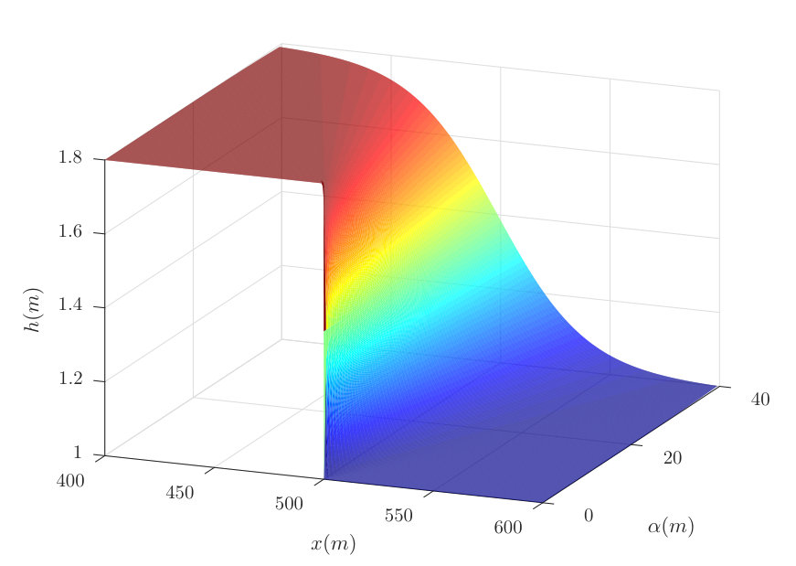 Figure 1
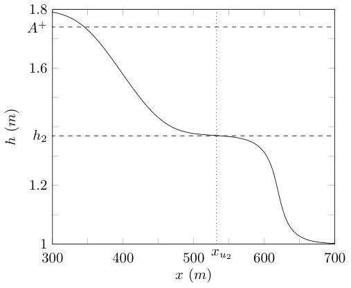 Figure 10
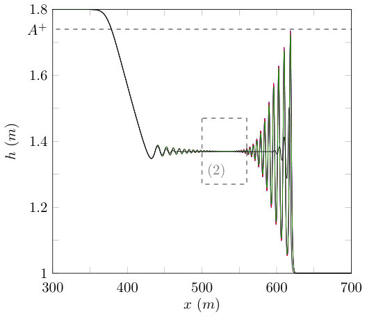 Figure 11
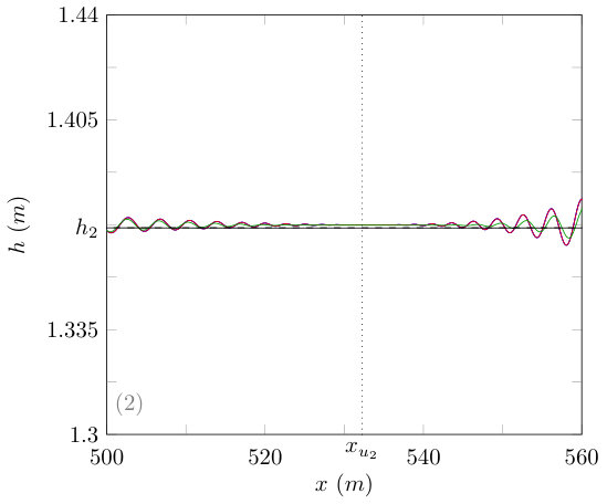 Figure 12
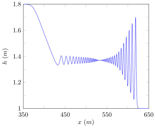 Figure 13
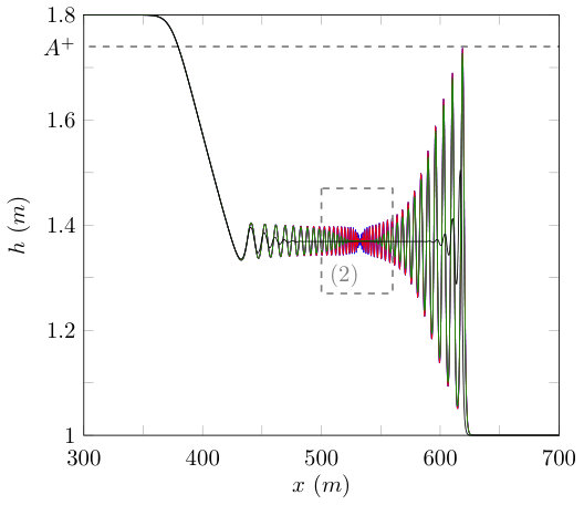 Figure 14
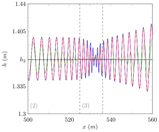 Figure 15
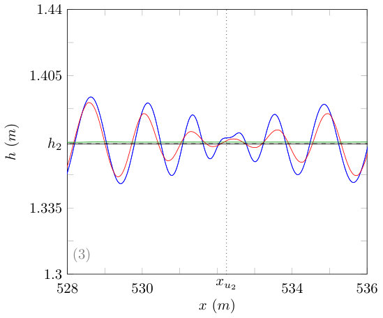 Figure 16
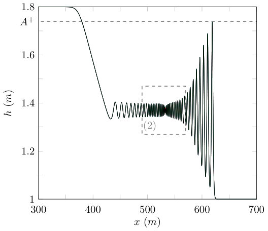 Figure 17
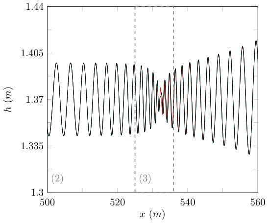 Figure 18
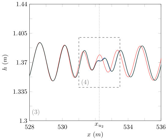 Figure 19
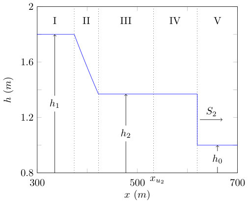 Figure 2
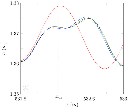 Figure 20
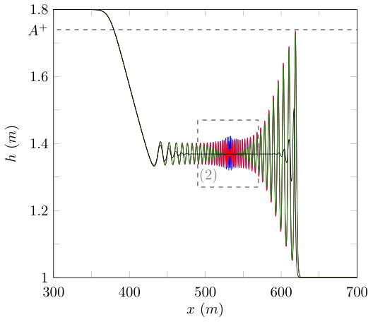 Figure 21
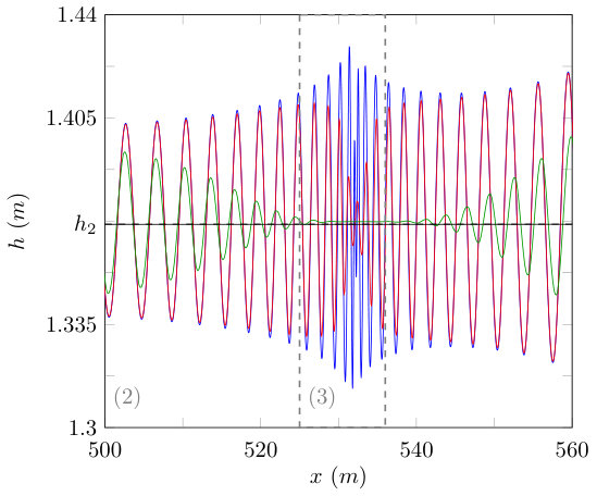 Figure 22
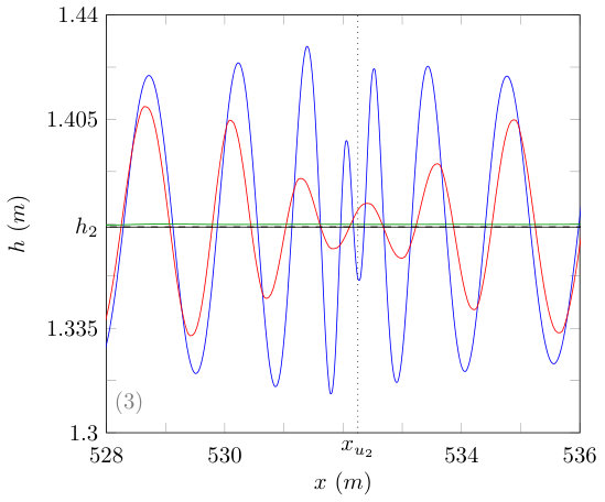 Figure 23
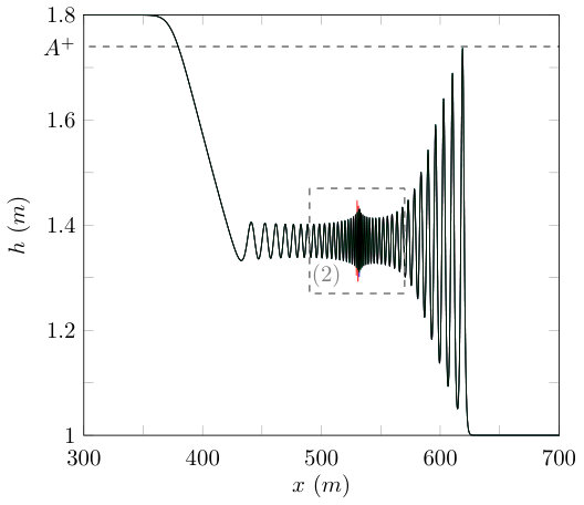 Figure 24
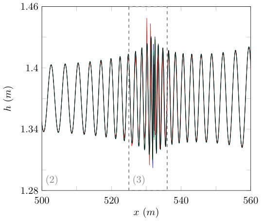 Figure 25
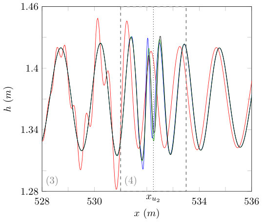 Figure 26
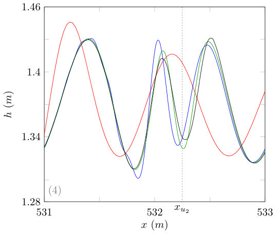 Figure 27
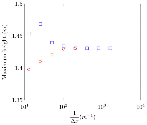 Figure 28
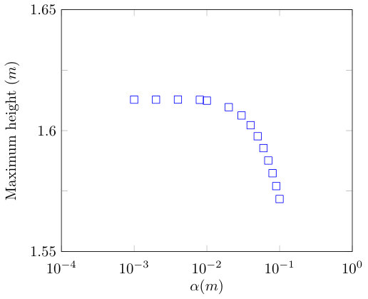 Figure 29
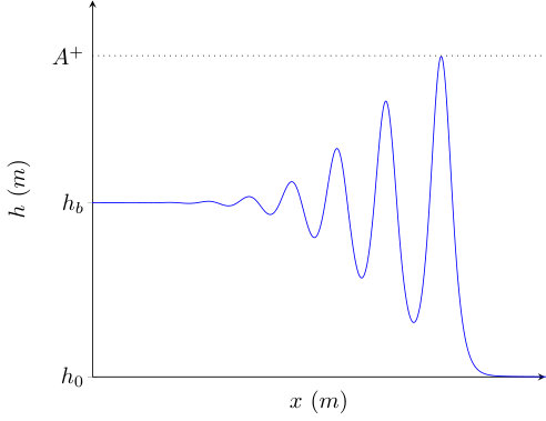 Figure 3
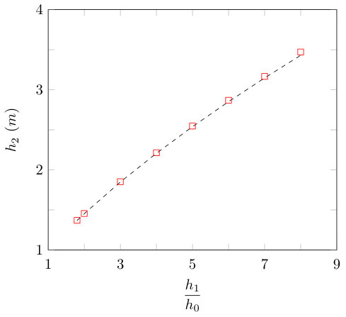 Figure 30
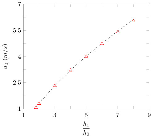 Figure 31
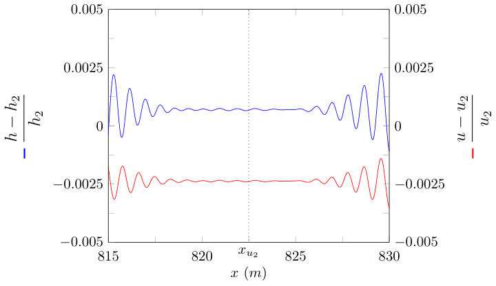 Figure 32
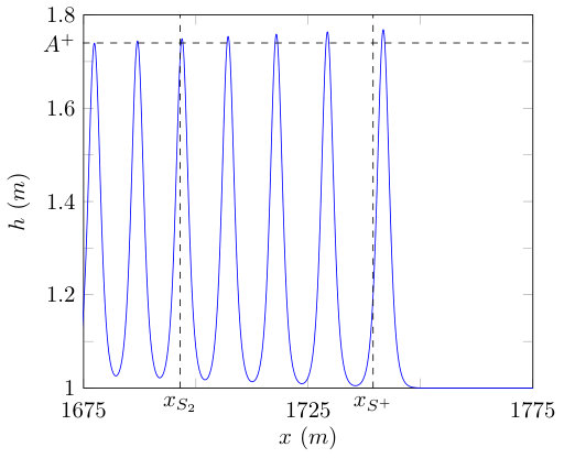 Figure 33
 Figure 34
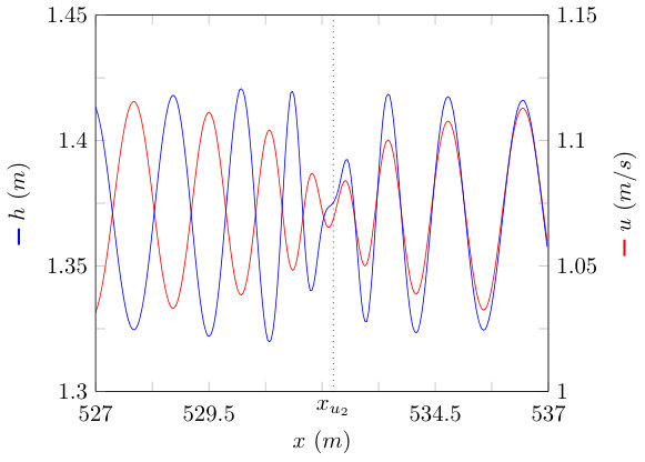 Figure 35
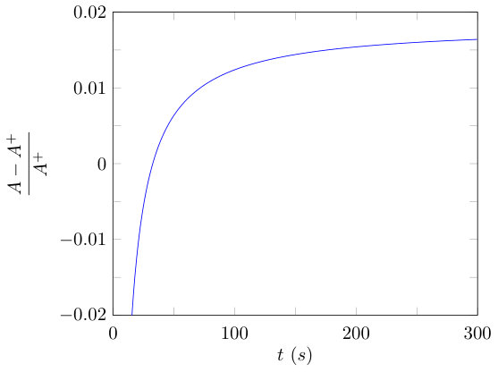 Figure 36
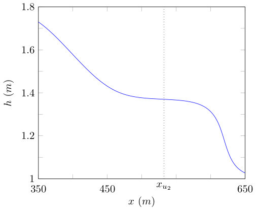 Figure 4
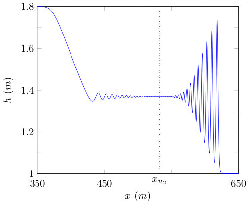 Figure 5
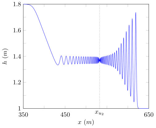 Figure 6
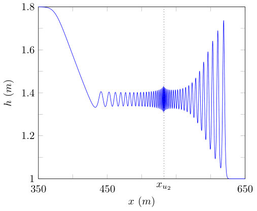 Figure 7
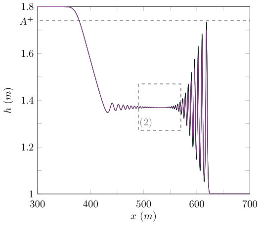 Figure 8
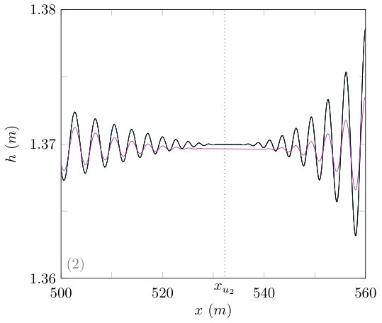 Figure 9
Peer Reviews
No public reviews on file for this paper yet. If you reviewed it on a platform where reviews are public (OpenReview, ICLR, NeurIPS, ICML), you can paste yours below so the community can read it here.
Videos
No videos yet. Explain this paper in a talk, walkthrough, or lecture? Add one.
Behaviour of the Serre Equations in the Presence of Steep Gradients Revisited
J.P.A. Pitt
C. Zoppou
S.G. Roberts
Mathematical Sciences Institute, Australian National University, Canberra, ACT 0200, Australia
Abstract
We use numerical methods to study the behaviour of the Serre equations in the presence of steep gradients because there are no known analytical solutions for these problems. In keeping with the literature we study a class of initial condition problems that are a smooth approximation to the initial conditions of the dam-break problem. This class of initial condition problems allow us to observe the behaviour of the Serre equations with varying steepness of the initial conditions. The numerical solutions of the Serre equations are justified by demonstrating that as the resolution increases they converge to a solution with little error in conservation of mass, momentum and energy independent of the numerical method. We observe four different structures of the converged numerical solutions depending on the steepness of the initial conditions. Two of these structures were observed in the literature, with the other two not being commonly found in the literature. The numerical solutions are then used to assess how well the analytical solution of the shallow water wave equations captures the mean behaviour of the solution of the Serre equations for the dam-break problem. Lastly the numerical solutions are used to evaluate the usefulness of asymptotic results in the literature to approximate the depth and location of the front of an undular bore.
keywords:
Serre equations, steep gradients , dam break
1 Introduction
The behaviour of flows containing steep gradients are important to a range of problems in shallow water such as the propagation of a bore, the dam-break problem and shoaling waves on a beach.
The Serre equations are used as a compromise between the non-dispersive shallow water wave equations and the incompressible inviscid Euler equations for modelling dispersive waves of the free surface in the presence of steep gradients, which are present for the Euler equations [1] but not for the shallow water wave equations. The Serre equations like the shallow water wave equations produce methods [2, 3, 4] that are computationally easier and quicker to solve than the best methods for the Euler equations. The Serre equations are considered the most appropriate approximation to the Euler equations for modelling dispersive waves up to the shore line [5, 6]. Therefore, understanding the behaviour of the Serre equations in the presence of steep gradients offers some insight into the behaviour of steep gradients for fluids more generally.
There are no known analytical solutions to problems containing steep gradients for the Serre equations. To infer the structure of solutions to problems containing steep gradients we have to resort to investigating numerical solutions of the Serre equations for these problems.
There are few examples in the literature which depict the behaviour of numerical solutions to the Serre equations in the presence of steep gradients [7, 2, 8, 1, 3, 4]. These papers all present problems with discontinuous initial conditions [2, 3, 4] or a smooth approximation to them when the numerical method requires some smoothness of the solutions [7, 8, 1]. Among these papers there are differences in the structures of the numerical solutions, with some demonstrating undulations in depth and velocity throughout the bore [7, 3, 4] and others showing a constant depth and velocity state in the middle of the bore [2, 8, 1].
The mean behaviour of numerical solutions to the dam-break problem for the Serre equations is consistent across the literature [7, 3, 4, 2, 8, 1] and was demonstrated to be well approximated by the analytical solution to the dam-break problem by the shallow water wave equations [2, 8]. Expressions for the leading wave amplitude and speed of an undular bore for the Serre equations were derived and verified for a range of undular bores by El et al. [7]. These expressions were also shown to be valid for all the different structures found in the literature [7, 8].
The first aim of this paper is to investigate and explain why different behaviour has been published in the literature for numerical solutions of the Serre equations for problems containing steep gradients. We find that the undulations of a bore can be damped to a constant depth and velocity state by the numerical diffusion introduced by the method, as is the case for Le Métayer et al. [2]. Oscillation damping can also occur due to the particular smoothing of the initial conditions, as is the case for Mitsotakis et al. [1], El et al. [7] and Mitsotakis et al. [8]. We do find that over long time periods the Serre equations damp these oscillations as they propagate, but this natural decay is dominated by other factors in the literature.
The second aim of this paper is to assess the utility of the shallow water wave equations and the results of El et al. [7] as guides for the evolution of an undular bore. We find that for a range of dam-break problems the analytical solution of the shallow water wave equations is a good approximation for the mean depth and velocity of the Serre equations, extending the findings of Le Métayer et al. [2] and Mitsotakis et al. [8] to a larger range of dam-break problems. It was also found that the results of El et al. [7] are a good approximation to our numerical solutions.
The first aim of this paper is achieved by demonstrating that our numerical solutions are good approximations to the true solutions of the Serre equations. This is accomplished by demonstrating that as the resolution of a particular method is increased, the numerical solutions converge to a numerical solution with little error in the conservation of mass, momentum and energy. The numerical solution is also consistent across the five different numerical methods. Three of the methods are the first, second and third-order methods presented by Zoppou et al. [4]. The first-order method is equivalent to the method of Le Métayer et al. [2]. The fourth method is a recreation of the second-order method used by El et al. [7]. Lastly, the fifth method is a second-order finite difference approximation to the Serre equations.
The second aim is accomplished by comparing our verified numerical solutions to the analytical solutions of the shallow water wave equations and the Whitham modulation results presented by El et al. [7].
The paper is organised as follows, in Section 2 the Serre equations and the quantities they conserve are presented. In Section 3 the smoothed dam-break problem is defined, the measures of the relative difference between numerical solutions and the relative error in the conserved quantities are presented. The analytical solution of the shallow water wave equations and the expressions for the amplitude and speed of the leading wave of an undular bore are presented. In Section 4 the numerical methods and their important properties are presented. In Section 5 the four different structures in the solutions of smoothed dam-break problem for the Serre equations are determined using verified numerical solutions. The verified numerical solutions are also used to evaluate how well the analytical solution of the shallow water wave equations captures the mean behaviour of the solution of the Serre equations for the dam-break problem. The Whitham modulations results are also compared to the verified numerical solutions to test their veracity.
2 Serre Equations
The Serre equations can be derived by integrating the full inviscid incompressible Euler equations over the water depth [9]. They can also be derived as an asymptotic expansion of the Euler equations [10]. Assuming a constant horizontal bed, the one-dimensional Serre equations are [11]
[TABLE]
Where is the horizontal velocity over the depth of water , is the acceleration due to gravity, is the horizontal spatial variable and is time.
The Serre equations are conservation laws for ‘mass’ (1a), ‘momentum’ (1b) and the Hamiltonian [12, 13]
[TABLE]
which is the total energy.
The total amount of a quantity in a system in the spatial interval at a particular time , is measured by
[TABLE]
Conservation of a quantity implies that for all provided the interval is fixed and the system is closed. Our numerical methods should demonstrate conservation for the quantities , and .
3 Smoothed Dam Break Problem
In this section we define a class of initial condition problems, called the smoothed dam-break problem that we use throughout our numerical investigation. This class of initial conditions are used in the literature [8, 1] to smoothly approximate the discontinuous initial conditions of the dam-break problem, as some numerical methods require smoothness of the solutions.
The smoothed dam-break problem has the following initial conditions
[TABLE]
This represents a smooth transition centred around between a water depth of on the right which is smaller than the water depth of on the left. Here measures the distance over which approximately of that smooth transition between the two heights occurs. Decreasing increases the steepness of the initial conditions as can be seen in Figure 1 where and . These are the same and values as those of the smoothed dam-break problem of El et al. [7] and the dam-break problem of Le Métayer et al. [2].
There are no known analytical solutions of the Serre equations for the dam-break problem or an arbitrary smoothed dam-break problem. Therefore, to demonstrate that our numerical solutions converge we use the relative difference between numerical solutions. To demonstrate that our numerical solutions also have small errors in the conserved quantities we use the relative error of their conservation. Both of these measures are defined in this section.
3.1 Assessing validity of Numerical Solutions
To demonstrate that our numerical solutions converge to a solution with little error in the conserved quantities as the spatial resolution is increased we use two measures; the relative difference between numerical solutions of different resolutions and the error in the conservation of a quantity. The relative difference between numerical solutions measures their convergence, while the error in conservation measures how well the numerical solutions conserve the quantities , and .
We introduce the following notation for the spatial grids defined by and the temporal grids defined by upon which the numerical solutions are calculated. These grids are uniform so that for all and for all . We use subscripts and superscripts to denote where a quantity is evaluated in the following way . Finally, the th cell is the interval [,] centred around .
3.1.1 Convergence of Numerical Results
To measure the convergence of the numerical solutions we ensured all grids had common locations to compare them by dividing by to create finer grids. Therefore, the finest grid with the smallest contains all the locations in any coarser grid. To measure the relative difference between quantities on these grids we compare them only on the coarser grid points . For some quantity we have our numerical approximation to it on the finest grid and on the coarser grid , with the relative difference between the two being
[TABLE]
3.1.2 Conserved Quantities
To calculate the error in conservation of a quantity, we must first calculate the total amount of the conserved quantities for the initial conditions. For the smoothed dam-break problem the initial conditions (3) were integrated to obtain expressions for the total mass , the total momentum and the total Hamiltonian . Provided is the midpoint of the spatial domain the total amounts for the conserved quantities are
[TABLE]
To calculate how well we approximate the total amount of a quantity in our numerical solution we fit a quartic interpolant of the primitive variables and over a cell utilising neighbouring cells and then apply Gaussian quadrature with 3 points. The amount of in each cell is summed across all cells to get the total amount of in our numerical solution at time , which we call . The error in conservation of a quantity for a numerical solution is
[TABLE]
Note that for the denominator is [math] and that there is a flux of momentum due to the unequal heights at both ends of the domain. To resolve this issue for the error in the conservation of is measured by
[TABLE]
3.2 Background for derived and observed comparisons
It was demonstrated by Le Métayer et al. [2] and Mitsotakis et al. [8] that the analytical solution of the shallow water wave equations for the dam-break problem captures the mean behaviour of the numerical solutions of the Serre equations to the dam-break problem [2] and the smoothed dam-break problem [8].
El et al. [7] derived an expression for the long term amplitude of the leading wave of an undular bore for the Serre equations. Since the front of an undular bore decomposes into solitons, the speed of the leading wave can be calculated from its amplitude.
To be self contained we present the analytical solution of the shallow water wave equations to the dam-break problem and the expressions derived by El et al. [7].
3.2.1 Shallow Water Wave Equation Analytical Solution
For the dam-break problem the shallow water wave equations, which are the Serre equations with dispersive terms neglected, can be solved analytically.
An example of the analytical solution of the shallow water wave equations for the dam-break problem is presented in Figure 2. Region I is the undisturbed water upstream of the dam-break at constant height () and velocity (). Region II is the rarefaction fan connecting regions I and III. Regions III and IV represent the shock with constant height () and constant velocity (), these regions are separated by . Region V is the undisturbed water downstream at constant height () and velocity () separated from Region IV by a shock which travels at velocity . Expressions for the unknown quantities , and in terms of and were given by Wu et al. [14] as
[TABLE]
Applying (8) to our dam-break heights of interest; and results in , and which are shown in Figure 2 for . The location of the front of the bore for the shallow water wave equations at time is thus so that .
3.2.2 Whitham Modulation for Undular Bores of the Serre Equations
Utilizing Whitham modulation theory for a one-phase periodic travelling wave an asymptotic analytical expression for the amplitude and speed of the leading wave was derived by El et al. [7]. An example of an undular bore is shown in Figure 3. The derived expressions for and are
[TABLE]
where , and is the height of the bore. The height of the bore created by the dam-break problem in (9a) used by El et al. [7] was
[TABLE]
For our dam-break heights of interest and we obtain , , and . The location of the leading wave of an undular bore at time is then so that .
4 Numerical Methods
Five numerical schemes were used to investigate the behaviour of the Serre equations in the presence of steep gradients, the first (), second () and third-order () finite difference finite volume methods of Zoppou et al. [4], the second-order finite difference method of El et al. [7] () and a second-order finite difference method () that can be found in the Appendix.
The methods are stable under a Courant-Friederichs-Lewy (CFL) condition presented by A. Harten [15]. The methods have demonstrated the appropriate order of convergence for smooth problems [4]. Furthermore, and have been validated against experimental data containing steep gradients [4]. The two methods and were found to be stable under the same CFL condition.
Generally, we found that is the worst performing method due to its numerical diffusion [4]. Of the high-order methods is the worst performing, introducing dispersive errors.
5 Numerical Results
We investigate the behaviour of the Serre equations in the presence of steep gradients by numerically solving the smoothed dam-break problem while varying the steepness of the initial conditions. As our numerical solutions should represent a good approximation of the true solution of the Serre equations. If our numerical solutions to a smoothed dam-break problem converge to the same numerical solution with little error in conservation of mass, momentum and energy as for each method, then this numerical solution is considered an accurate approximate solution to that smoothed dam-break problem for the Serre equations.
This process validates our numerical solutions for the smoothed dam-break problem, and thus validates our numerical methods to approximate the solution of the Serre equations in the presence of steep gradients, if it exists. With a validated model we can compare the numerical solution to the analytical solution of the shallow water wave equations for the dam-break problem and the results of El et al. [7].
Throughout most of this section we are interested in the numerical solution at to the smoothed dam-break problem with , and while allowing for different values. All numerical methods used which is smaller than required by the CFL condition, ensuring stability of our schemes. The method requires an input parameter to its slope limiter and this was chosen to be [4]. The spatial domain was with the following Dirichlet boundary conditions, at both boundaries, on the left and on the right.
5.1 Observed Structures of the Numerical Solutions
We observe that there are four different structures for the converged to numerical solution depending on the chosen . They are the ‘non-oscillatory’ structure , the ‘flat’ structure , the ‘node’ structure and the ‘growth’ structure . An example of each of these structures is shown in Figure 4 which were obtained using with .
The four structures are identified by the dominant features of the numerical solutions in regions III and IV. They also correspond to different structures in the numerical solutions that have been presented in the literature. From Figure 4 it can be seen that as is decreased, steepening the initial conditions, the numerical solutions demonstrate an increase in the size and number of oscillations particularly around . We observe that the difference between , and is the amplitude of the oscillations in regions III and IV.
For the non-oscillatory and flat structures there is excellent agreement between all higher-order numerical methods at our highest resolution . An illustration of this agreement is given in Figure 5 for which is the most difficult to resolve of the two structures. However, the first-order method suppresses oscillations present in the numerical solutions of other methods due to its diffusive errors [4]. To resolve these oscillations with much lower of values of are required.
5.1.1 Non-oscillatory Structure
The “non-oscillatory” structure is the result of a large , which causes the front of this flow to not be steep enough to generate undulations over short time periods. As the system evolves the front will steepen due to non-linearity and undulations will develop.
The structure is not present in the literature as no authors chose large enough because, such a large poorly approximates the dam-break problem. An example of this structure can be seen in Figure 6 for using with various values. Because this is not a very steep problem all numerical results are visually identical for all .
From Table 1 it can be seen that not only have these solutions converged visually but the measures demonstrate that we have reached convergence to round-off error by after which the relative difference between numerical solutions plateau.
Table 1 also demonstrates that the error in conservation of the numerical solutions are at round-off error for and . The conservation of is poor because the smoothed dam-break has such a large that and , causing unequal fluxes in momentum at the boundaries.
As stated above when the numerical solutions from all methods are identical for this smoothed dam-break problem.
The convergence of the numerical solutions as to a numerical solution with small error in conservation, independent of the method demonstrates that we have accurately solved the smoothed dam-break problem with . Therefore, the structure should be observed in the solutions of the Serre equations for the smoothed dam-break problem for sufficiently large .
5.1.2 Flat Structure
The most common structure observed in the literature [2, 8, 1] is the “flat structure” . It is observed when the initial conditions are steep enough such that the bore that develops has undulations. This structure consists of oscillations in regions III and IV which are separated by a constant height state around . An example of the structure can be seen in the numerical solutions presented in Figure 7 where .
As decreases the numerical solutions converge so that by the solutions for higher are visually identical. Table 1 demonstrates that although we have convergence visually, the measures are still decreasing and are larger than round-off error. Likewise the measures are still decreasing and have only reached round-off error for . This indicates that to attain full convergence of the numerical solutions of this smoothed dam-break problem down to round-off error using would require an even smaller . The relative difference between numerical solutions is small and the numerical solutions exhibit good conservation. Therefore, our highest resolution numerical solution is a good approximation to any numerical solutions with lower values. Figure 5 demonstrates that at the numerical solutions of all higher order methods are the same.
These results demonstrate that our highest resolution numerical solution is an accurate approximate solution of the Serre equations for the smoothed dam-break problem with . This implies that the structure should be observed in solutions of the Serre equations for smooth dam-break problems with similar values.
These numerical solutions compare well with those of Mitsotakis et al. [8] who use the same but different and values and observe the structure. We found that we observed this structure for all numerical method’s numerical solutions to the smoothed dam-break problem with values as low as and . The numerical solutions of Mitsotakis et al. [1] use but different heights and observe the structure . Therefore Mitsotakis et al. [1] and Mitsotakis et al. [8] observe the structure in their numerical results due to their choice of for the smoothed dam-break problem.
The first-order method is diffusive [4] and damps oscillations that are present in the numerical solutions of higher-order methods as in Figure 5. We find that for any smoothed dam-break problem with and the dam-break problem only the structure is observed for the numerical solutions of at with . This is evident in Figure 8 with the numerical solutions of using our finest grid where on our steepest initial conditions where . Therefore, Le Métayer et al. [2] using the diffusive with their chosen and , which are larger than our and could only observe the structure.
5.1.3 Node Structure
The “node” structure, was observed by El et al. [7]. The structure has oscillations throughout regions III and IV that decay to a node at as can be seen in Figure 9 where .
Figure 9 demonstrates that our numerical solutions have not converged, however this is only in the area around . Due to the large difference in numerical solutions around the measure over the area around would not be insightful. However, by omitting this region we can gain some knowledge about how well our solutions agree away from . This was performed for the relevant measures in Table 1 by omitting the interval [, ]. These modified measures demonstrate that while our numerical results have visually converged outside this interval, they have not converged down to round-off error.
Table 1 demonstrates that the measures are still decreasing and have only attained round-off error for . Therefore, to resolve the desired convergence of the numerical solutions to one with small error in conservation using would require even smaller values.
There is good agreement across different numerical methods for as can be seen in Figure 10. In particular all the higher-order methods exhibit the same structure and only disagree in a very small region around . We observe that the numerical solution of the worst higher-order method has not converged well to the numerical solutions of the other higher-order methods.
We have only obtained a good approximation to the desired numerical solution as away from . However, our highest resolution numerical solutions from various higher-order methods are very similar. This suggests that again although we do not have full convergence, our highest resolution numerical solution is a good approximation to the desired numerical solution over the whole domain. Therefore, our highest resolution numerical solutions are an accurate representation of the solutions of the Serre equations for this smoothed dam-break problem. Therefore, the structure should be observed in the solutions of the Serre equations for the smoothed dam-break problem with .
These numerical solutions support the findings of El et al. [7] who also use some smoothing [16] but do not report what smoothing was performed. Using their method and similar to El et al. [7] we observe the “growth” structure in the numerical solution for values smaller than , indicating that the smoothing performed by El et al. [7] limited their observed behaviour to just the structure.
5.1.4 Growth Structure
The “growth” structure, which has hitherto not been commonly published in the literature features a growth in the oscillation amplitude around . An example of the growth structure can be seen for ’s numerical solutions in Figure 11 to the smoothed dam-break problem with . This structure was observed in the numerical solutions of for at for values as low as and even for the dam-break problem.
Figure 11 shows that this structure can only be observed for , with poor convergence of the numerical results around . Again our measures in Table 1 omit the interval [,] in the numerical solutions. This demonstrates that although we have visual convergence away from our numerical solutions have not converged to round-off error as . The measures in Table 1 are still decreasing and have only attained round-off error for , although for and the errors in conservation are small. These measures continue the trend in Table 1 where smaller ’s and thus steeper initial conditions lead to larger and measures because steeper problems are more difficult to solve accurately.
Figure 12 demonstrates that our numerical solutions for with the best methods , and disagree for only a few oscillations around . Since both and are second-order finite difference methods their errors are dispersive. These dispersive errors cause the numerical solutions to overestimate the oscillation amplitude of the true solution, particularly around . Because the dispersive errors of are larger than more oscillations are observed for the numerical solutions produced by . The method was shown to be diffusive by Zoppou et al. [4] and therefore its numerical solutions underestimate the oscillation amplitude in the true solution. Therefore, the true solution of the Serre equations should be between the dispersive method and the diffusive method , and thus will possess the structure.
The numerical solutions of and acting as upper and lower bounds respectively for the oscillation amplitude as is reduced is demonstrated in Figure 13 using the maximum of in the interval [, ]. From this figure it is clear that the amplitudes of the numerical solutions of converge down to the limit as the resolution is increased while the numerical solution amplitudes of converge up to it. This shows that we have effectively bounded the true solution of the Serre equations. Unfortunately, could not be run in reasonable computational times with lower , but the numerical solutions of show that doing so is unnecessary.
These results indicate that the solutions of the Serre equations to the smoothed dam-break problem with sufficiently small values should exhibit a growth structure at , even though we have not precisely resolved all the oscillations in our numerical solutions.
It was found that decreasing did increase the amplitude of the oscillations around . For with and the oscillations in were bounded by the interval [,]. Of particular note is that the number of oscillations are the same in Figures 10 and 12 for the best methods even though they have different structures.
By changing the interval and desired time for the numerical solution, could be lowered further so that by our numerical solutions have fully converged for values as low as . This allows us to show that the height of the oscillations around for the solution of the Serre equation to the smoothed dam-break problem are bounded at as . Figure 14 demonstrates this for the numerical solutions of with .
5.2 Shallow water wave equation comparison
The analytical solutions of the shallow water wave equations have been used as a guide for the mean behaviour of the solution of the Serre equations for the dam-break problem in the literature [2, 8].
To assess the applicability of this the mean bore depth and mean fluid velocity in the interval [,] were calculated from our numerical solution to the smoothed dam-break problem with various height ratios. These means were compared to their approximations from the analytical solution of the dam-break problem for the shallow water wave equations and . The results of this can be seen in Figure 15 for numerical solutions of with to the smoothed dam-break problem at with where is fixed and is varied.
We use a final time of as it allows the internal structure of the bore to develop more fully giving a more reliable mean estimate, as a consequence we resort to a coarser grid to keep the run-times reasonable. We find that decreasing does not significantly alter the mean of and . We also find that increasing also does not significantly alter the mean of and . Therefore, the mean behaviour of the true solution of the Serre equations to the dam-break problem is captured by these numerical solutions, if it exists.
It can be seen that and are good approximations to the mean behaviour of the fluid inside the bore for a range of different aspect ratios. Although, as increases this approximation becomes worse, so that becomes an underestimate and consequently is an overestimate.
We find that for the mean values of and inside the bore for the Serre equations are not equal to and . This can be seen in Figure 16 for the numerical solutions of with to the smoothed dam-break problem with at . It can be seen that is an underestimate of and is an overestimate of although the difference between these values and the mean behaviour of the Serre equations is small and only noticeable over long time periods.
The location of the leading wave of the Serre equations slowly diverges from the location of the front of a bore in the shallow water wave equations over long periods of time. This divergence causes the small difference evident in ’s numerical solution to the smoothed dam-break problem with at using , which is shown in Figure 17.
We note that the structure present in the numerical solutions using this method and parameters at in Figure 11 has decayed away by in Figure 16. This is a trend throughout our numerical solutions where oscillation amplitude decreases over time around , changing the structure of the solution. This can be seen by obtaining full convergence of the numerical solutions to the smoothed dam-break problem at . The converged to numerical solutions for are shown in Figure 18. From this figure it can be seen that the oscillation amplitudes for the numerical solutions for the smoothed dam-break problems with and are much larger at than they are at in Figure 4. Since we have demonstrated that our numerical solutions are good approximations to the true solution of the Serre equations at and , decreasing oscillation amplitude around over time is probably a property of the Serre equations. This implies that bounding the oscillation amplitudes at time as was done above, bounds the oscillation amplitudes at all later times.
5.2.1 Contact discontinuity
El et al. [7] noted the presence of a ‘degenerate contact discontinuity’ which is the node in the structure and travels at the mean fluid velocity in the bore.
We observe that as our numerical solutions evolve over time, oscillations appear to be released from the contact discontinuity and travel away from it in both directions, leading to decay of amplitudes around the contact discontinuity. Therefore, the contact discontinuity is an important feature and its behaviour determines the structure of the oscillations in the middle of the undular bore.
The different speeds of the oscillations are determined by the phase velocity, which for the Serre equations linearised around the mean height and mean velocity in regions III and IV of the solution to the dam-break problem is
[TABLE]
with wave number . It can be seen that as then and as then . Since the contact discontinuity travels at the mean velocity inside the bore, it corresponds to very high wave number oscillations. The oscillations on the left travel slower than the contact discontinuity and are therefore lower wave number oscillations associated with the phase velocity . The oscillations on the right travel travel quicker than the contact discontinuity and are therefore lower wave number oscillations associated with the phase velocity .
These different phase velocities have two different behaviours for and . When the phase velocity is we have oscillations where and are in-phase, while when the phase velocity is we have oscillations where and are out-of-phase. This can be seen in Figure 19 for the numerical solutions of with for the smoothed dam-break problem with at .
5.3 Whitham Modulation Comparsion
El et al. [7] demonstrated that their Whitham modulation results approximated the numerical solutions of the smoothed dam-break problem well for a range of aspect ratios. We observed that the Whitham modulation results are an underestimate compared to our numerical solutions.
This can be seen in Figure 20 as the relative difference between from El et al. [7] and the leading wave amplitude of our numerical solution does not converge to [math] over time. Since we find that the numerical solutions for the smoothed dam-break problem with have converged for the front of the undular bore by as in Figure 11, our numerical solutions for are considered reliable. We also note that unlike the oscillations around the leading wave amplitude increases over time.
The Whitham modulation results for the location of the leading wave is a better approximation than that given by the shallow water wave equations , as can be seen in Figure 17.
6 Conclusions
Utilising two finite difference methods of second-order and three finite difference finite volume methods of various orders to solve the nonlinear weakly dispersive Serre equations an investigation into the smoothed dam-break problem with varying steepness was performed. Four different structures of the numerical solutions were observed and demonstrated to be valid, the general trend of these structures is that an increase in steepness increases the size and number of oscillations in the solution. This study explains the different structures exhibited by the numerical results in the literature for the smoothed dam-break problem for the Serre equations and uncovers a new result. These results demonstrate that other methods in the literature could replicate our results if their simulations are extended. Furthermore, these results suggest that this new result and its associated structure is to be expected for the solution of the Serre equation to the dam-break problem at least for short enough time spans, if it exists.
We find that the analytical solution of the shallow water wave equations for the dam-break problem provides a reasonable approximation to the mean height and velocity inside the bore formed by the smoothed dam-break problem for the Serre equations. Finally, we observe that the Whitham modulations results for the leading wave of an undular bore provide a more accurate approximation to the location and depth of the front of an undular bore than the shallow water wave equations.
References
- Mitsotakis et al. [2017]
D. Mitsotakis, D. Dutykh, J. Carter, On the nonlinear dynamics of the traveling-wave solutions of the Serre system, Wave Motion 70 (1) (2017) 166–182.
- Le Métayer et al. [2010]
O. Le Métayer, S. Gavrilyuk, S. Hank, A numerical scheme for the Green-Naghdi model, Journal of Computational Physics 229 (6) (2010) 2034–2045.
- Zoppou et al. [2017a]
C. Zoppou, S. Roberts, J. Pitt, A Solution of the Conservation Law Form of the Serre Equations, The ANZIAM Journal 57 (4) (2017a) 385–394.
- Zoppou et al. [2017b]
C. Zoppou, J. Pitt, S. Roberts, Numerical Solution of the Fully Non-Linear Weakly Dispersive Serre Equations for Steep Gradient Flows, Applied Mathematical Modelling 48 (2017b) 70–95.
- Bonneton et al. [2011a]
P. Bonneton, E. Barthélemy, F. Chazel, R. Cienfuegos, D. Lannes, F. Marche, M. Tissier, Recent advances in Serre-Green Naghdi modelling for wave transformation, breaking and runup processes, European Journal of Mechanics B/Fluids 30 (6) (2011a) 589–597.
- Bonneton et al. [2011b]
P. Bonneton, F. Chazel, D. Lannes, F. Marche, M. Tissier, A splitting approach for the fully nonlinear and weakly dispersive Green-Naghdi model, Journal of Compuational Physics 230 (4) (2011b) 1479–1498.
- El et al. [2006]
G. El, R. H. J. Grimshaw, N. F. Smyth, Unsteady undular bores in fully nonlinear shallow-water theory, Physics of Fluids 18 (2) (2006) 027104.
- Mitsotakis et al. [2014]
D. Mitsotakis, B. Ilan, D. Dutykh, On the Galerkin/Finite-Element Method for the Serre Equations, Journal of Scientific Computing 61 (1) (2014) 166–195.
- Su and Gardner [1969]
C. H. Su, C. S. Gardner, Korteweg-de Vries equation and generalisations. III. Derivation of the Korteweg-de Vries equation and Burgers equation, Journal of Mathematical Physics 10 (3) (1969) 536–539.
- Lannes and Bonneton [2009]
D. Lannes, P. Bonneton, Derivation of asymptotic two-dimensional time-dependent equations for surface water wave propagation, Physics of Fluids 21 (1) (2009) 16601–16610.
- Li et al. [2014]
M. Li, P. Guyenne, F. Li, L. Xu, High order well-balanced CDG-FE methods for shallow water waves by a Green-Naghdi model, Journal of Computational Physics 257 (2014) 169–192.
- Li [2002]
Y. A. Li, Hamiltonian Structure and Linear Stability of Solitary Waves of the Green-Naghdi Equations, Journal of Nonlinear Mathematical Physics 9 (2002) 99–105.
- Green and Naghdi [1976]
A. E. Green, P. M. Naghdi, A derivation of equations for wave propagation in water of variable depth, Journal of Fluid Mechanics 78 (2) (1976) 237–246.
- Wu et al. [1999]
C. Wu, G. Huang, Y. Zheng, Theoretical solution of dam-break shock wave, Journal of Hydraulic Engineering 125 (11) (1999) 1210–1215.
- A. Harten [1983]
A. A. Harten, High resolution schemes for hyperbolic conservation laws, Journal of Computational Physics 49 (3) (1983) 357–393.
- El and Hoefer [2016]
G. El, M. Hoefer, Dispersive shock waves and modulation theory, Physica D: Nonlinear Phenomena 333 (2016) 11–65.
Appendix A
The methods and use the centred second-order finite difference approximation to the momentum equation (1b), denoted as . For the mass equation (1a) uses the two step Lax-Wendroff method, denoted as while uses a centred second-order finite difference approximation, denoted as .
A.1 for the Momentum Equation
First (1b) is expanded to get
[TABLE]
where contains only spatial derivatives and is
[TABLE]
All derivatives are approximated by second-order centred finite difference approximations on a uniform grid in space and time, which after rearranging into an update formula becomes
[TABLE]
where
[TABLE]
and
[TABLE]
Equation (11) can be rearranged into an explicit update scheme for given its current and previous values, so that
[TABLE]
where is a tri-diagonal matrix.
A.2 Numerical Methods for the Mass Equation
The two step Lax-Wendroff update for is
[TABLE]
[TABLE]
and
[TABLE]
The quantities are calculated using obtained by applying (18) to then linearly interpolating in space and time to give
[TABLE]
and
[TABLE]
Thus we have the following update scheme for (1a)
[TABLE]
The second order centered finite difference approximation to the conservation of mass equation (1a) is
[TABLE]
Thus we have an update scheme for all
[TABLE]
A.3 Complete Method
The method is the combination of (19) for (1a) and (18) for (1b) in the following way
[TABLE]
The method is the combination of (20) for (1a) and (18) for (1b) in the following way
[TABLE]
The reference list from the paper itself. Each links out to its DOI / PubMed record.
- 1Mitsotakis et al. [2017] D. Mitsotakis, D. Dutykh, J. Carter, On the nonlinear dynamics of the traveling-wave solutions of the Serre system, Wave Motion 70 (1) (2017) 166–182.
- 2Le Métayer et al. [2010] O. Le Métayer, S. Gavrilyuk, S. Hank, A numerical scheme for the Green-Naghdi model, Journal of Computational Physics 229 (6) (2010) 2034–2045.
- 3Zoppou et al. [2017 a] C. Zoppou, S. Roberts, J. Pitt, A Solution of the Conservation Law Form of the Serre Equations, The ANZIAM Journal 57 (4) (2017 a) 385–394.
- 4Zoppou et al. [2017 b] C. Zoppou, J. Pitt, S. Roberts, Numerical Solution of the Fully Non-Linear Weakly Dispersive Serre Equations for Steep Gradient Flows, Applied Mathematical Modelling 48 (2017 b) 70–95.
- 5Bonneton et al. [2011 a] P. Bonneton, E. Barthélemy, F. Chazel, R. Cienfuegos, D. Lannes, F. Marche, M. Tissier, Recent advances in Serre-Green Naghdi modelling for wave transformation, breaking and runup processes, European Journal of Mechanics B/Fluids 30 (6) (2011 a) 589–597.
- 6Bonneton et al. [2011 b] P. Bonneton, F. Chazel, D. Lannes, F. Marche, M. Tissier, A splitting approach for the fully nonlinear and weakly dispersive Green-Naghdi model, Journal of Compuational Physics 230 (4) (2011 b) 1479–1498.
- 7El et al. [2006] G. El, R. H. J. Grimshaw, N. F. Smyth, Unsteady undular bores in fully nonlinear shallow-water theory, Physics of Fluids 18 (2) (2006) 027104.
- 8Mitsotakis et al. [2014] D. Mitsotakis, B. Ilan, D. Dutykh, On the Galerkin/Finite-Element Method for the Serre Equations, Journal of Scientific Computing 61 (1) (2014) 166–195.