On risk averse competitive equilibrium
Henri G\'erard (CERMICS), Vincent Lecl\`ere (CERMICS), Andy Philpott

TL;DR
This paper explores risk-averse competitive equilibrium models where agents use coherent risk measures, revealing non-uniqueness of equilibria and limitations of standard computational methods in finding all solutions.
Contribution
It demonstrates that risked equilibria are not unique and highlights the challenges of computational methods in capturing all equilibrium outcomes.
Findings
Risked equilibria are not unique even with strictly concave objectives.
Standard computational methods may only find a subset of equilibria.
Risk measures significantly impact equilibrium analysis.
Abstract
We discuss risked competitive partial equilibrium in a setting in which agents are endowed with coherent risk measures. In contrast to socialplanning models, we show by example that risked equilibria are not unique, even when agents' objective functions are strictly concave. We also show that standard computational methods find only a subset of the equilibria, even with multiple starting points.
Click any figure to enlarge with its caption.
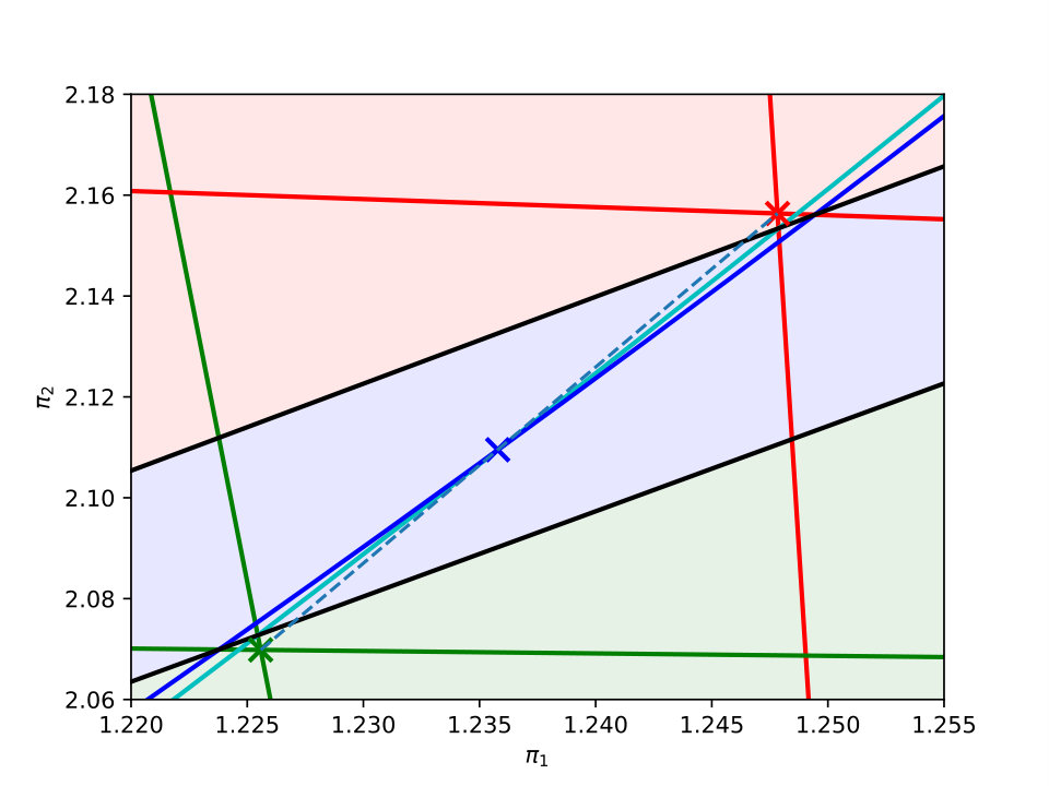 Figure 1
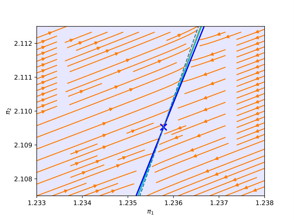 Figure 2
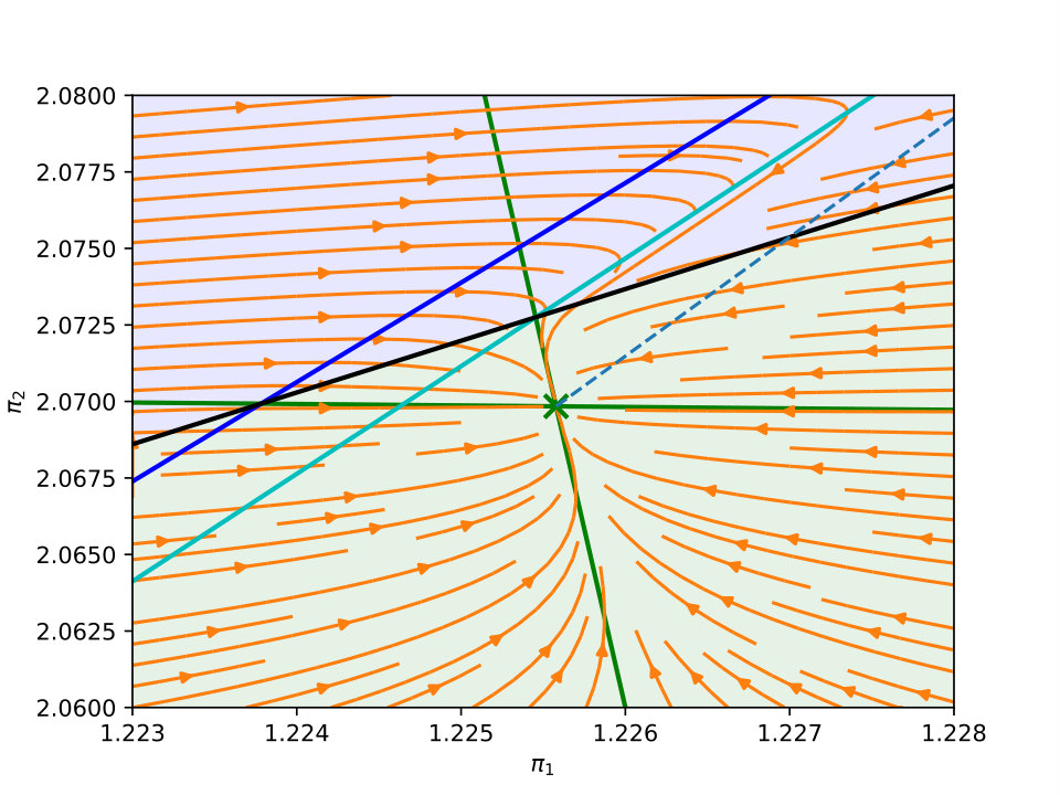 Figure 3
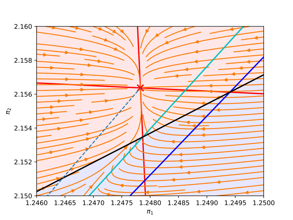 Figure 4
| condition | ||||
|---|---|---|---|---|
| case a) | ||||
| case b) | ||||
| case c) |
| condition | ||||
|---|---|---|---|---|
| case a) | ||||
| case b) | ||||
| case c) |
Peer Reviews
No public reviews on file for this paper yet. If you reviewed it on a platform where reviews are public (OpenReview, ICLR, NeurIPS, ICML), you can paste yours below so the community can read it here.
Videos
No videos yet. Explain this paper in a talk, walkthrough, or lecture? Add one.
On risk averse competitive equilibrium
Henri Gerard
Université Paris-Est, CERMICS (ENPC), F-77455 Marne-la-Vallée, France
Electric Power Optimization Centre, The University of Auckland, New Zealand
Université Paris-Est, Labex Bézout, F-77455 Marne-la-Vallée, France
Vincent Leclere
Andy Philpott
Abstract
We discuss risked competitive partial equilibrium in a setting in which agents are endowed with coherent risk measures. In contrast to social planning models, we show by example that risked equilibria are not unique, even when agents’ objective functions are strictly concave. We also show that standard computational methods find only a subset of the equilibria, even with multiple starting points.
keywords:
Stochastic Equilibrium , Stochastic Programming , Risk averse equilibrium , Electricity Markets
††journal: Operations Research Letters
1 Introduction
Most industrialised regions of the world have over the last thirty years established wholesale electricity markets that take the form of an auction that matches supply and demand. The exact form of these auction mechanisms vary by jurisdiction, but they typically require offers of energy from suppliers at costs they are willing to supply, and clear a market by dispatching these offers in order of increasing cost. Day-ahead markets such as those implemented in many North American electricity systems, seek to arrange supply well in advance of its demand, so that thermal units can be prepared in time. Since the demand cannot be predicted with absolute certainty, day-ahead markets must be accompanied by a separate balancing market to deal with the variation in load and generator availability in real time. These are often called two-settlement markets. The market mechanisms are designed to be as efficient as possible in the sense that they should aim to maximize the total welfare of producers and consumers.
In response to pressure to reduce emissions and increase the penetration of renewables, electricity pool markets are procuring increasing amounts of electricity from intermittent sources such as wind and solar. If probability distributions for intermittent supply are known for these systems then it makes sense to maximize the expected total welfare of producers and consumers in each dispatch. Then many repetitions of this will yield a long run total benefit that is maximized. Maximizing expected welfare can be modeled as a two-stage stochastic program. Methods for computing prices and single-settlement payment mechanisms for such a stochastic market clearing mechanism are described in a number of papers (see Pritchard et al. [11], Wong and Fuller [16] and Zakeri et al. [17]). When evaluated using the assumed probability distribution on supply, stochastic market clearing can be shown to be more efficient than two-settlement systems.
If agents in these systems are risk averse then one might also seek to maximize some risk-adjusted social welfare. In this setting the computation of prices and payments to the agents becomes more complicated. If agents use coherent risk measures then it is possible to define a complete market for risk in a precise sense. If the market is complete then a perfectly competitive partial equilibrium will also maximize risk-adjusted social welfare, i.e. it is efficient. On the other hand if the market for risk is not complete, then perfectly competitive partial equilibrium can be inefficient. This has been explored in a number of papers (see e.g. de Maere d’Aertrycke et al. [4], Ehrenmann and Smeers [5] and Ralph and Smeers [12]).
In this paper we study a class of stochastic dispatch and pricing mechanisms under the assumption that agents will attempt to maximize their risk-adjusted welfare at these prices. Agents have coherent risk measures and are assumed to behave as price takers in the energy and risk markets. We aim at enlightening some difficulties that arise when risk markets are not complete. We describe a simple instance of a stochastic market that has three different equilibria. Two of these points are stable in the sense of Samuelson [13] and are attractors of tatônnement algorithms. The third equilibrium is unstable, yet is the solution yielded by the well-known PATH solver in GAMS (See Ferris and Munson [8]). Our example illustrates the delicacy of seeking numerical solutions for equilibria in incomplete markets. Since these are used for justifying decisions, the nonuniqueness of solutions in this setting is undesirable.
The paper is laid out as follow. In Section 2 we present the equilibrium and optimization models we are going to study. In Section 3 we give links between equilibrium and optimization problems in the risk neutral and complete risk-averse cases. Finally, in Section 4 we showcase a simple example with multiple equilibria in the incomplete risk-averse case.
1.1 Notation
We use the following notation throughout the paper: is the set of integers between and (included), random variables are denoted in bold, is a finite sample space, is a probability distribution over , is used to refer to expectation with respect to , is used to refer to a risk measure. We denote by the complementarity condition .
2 Statement of problem
Consider a two time-step single-settlement market for one good. In a single-settlement market, the producer can arrange in advance for a production of at a marginal cost as a first-step decision, and choose the value of a recourse variable incurring an uncertain marginal cost . We assume that there are a finite number of scenarios determining the coefficient .
The product is purchased in the second step by a consumer with a utility function . The consumer has no first-stage decision, and the amount purchased depends on the scenario.
2.1 Social planner problem
Decisions , and can be made to maximize a social objective. We denote by
[TABLE]
the welfare of the consumer where both these expressions ignore the price paid for the good in scenario . Then the welfare of the social planner can be defined by \boldsymbol{W^{\textstyle\text{\unboldmath\scriptstyle}}_{\textstyle\text{\unboldmath\scriptstyle sp}}}=\boldsymbol{W^{\textstyle\text{\unboldmath\scriptstyle}}_{\textstyle\text{\unboldmath\scriptstyle p}}}+\boldsymbol{W^{\textstyle\text{\unboldmath\scriptstyle}}_{\textstyle\text{\unboldmath\scriptstyle c}}}.
Optimization of the social objective requires us to aggregate the uncertain outcomes from the scenarios. This can be done by taking expectations with respect to an underlying probability measure or using a more general risk measure.
2.1.1 Risk neutral social planner problem
Endow the set of scenario with a probability , then a risk-neutral social planner might seek to maximize the expected total social welfare under the constraint that supply equals demand. This problem is denoted by and reads
[TABLE]
2.1.2 Risk averse social planner problem
Choosing expectation , assumes a risk-neutral point of view, where two random losses with same expectation but different variances are deemed equivalent. In practice a number of agents are risk averse. To model risk aversion we generally use a risk measure , that is a functional that associates to a random welfare its deterministic equivalent, i.e. the deterministic welfare deemed as equivalent to the random loss.
A risk-averse planner solves a maximization problem defined by
[TABLE]
A risk measure is said to be coherent (see Artzner et al. [2]) if it satisfies four natural properties: monotonicity ( if \boldsymbol{X^{\textstyle\text{\unboldmath\scriptstyle}}_{\textstyle\text{\unboldmath\scriptstyle}}}\geq\boldsymbol{Y^{\textstyle\text{\unboldmath\scriptstyle}}_{\textstyle\text{\unboldmath\scriptstyle}}} then \mathbb{F}[\boldsymbol{X^{\textstyle\text{\unboldmath\scriptstyle}}_{\textstyle\text{\unboldmath\scriptstyle}}}]\geq\mathbb{F}[\boldsymbol{Y^{\textstyle\text{\unboldmath\scriptstyle}}_{\textstyle\text{\unboldmath\scriptstyle}}}]), concavity ( is concave), translation-equivariance (\mathbb{F}[\boldsymbol{X^{\textstyle\text{\unboldmath\scriptstyle}}_{\textstyle\text{\unboldmath\scriptstyle}}}+c]=\mathbb{F}[\boldsymbol{X^{\textstyle\text{\unboldmath\scriptstyle}}_{\textstyle\text{\unboldmath\scriptstyle}}}]+c with ) and positive homogeneity (\mathbb{F}[\lambda\boldsymbol{X^{\textstyle\text{\unboldmath\scriptstyle}}_{\textstyle\text{\unboldmath\scriptstyle}}}]=\lambda\mathbb{F}[\boldsymbol{X^{\textstyle\text{\unboldmath\scriptstyle}}_{\textstyle\text{\unboldmath\scriptstyle}}}], with ). By convex duality theory (see Shapiro et al. [14]), a lower-semicontinuous coherent risk measure can be written \mathbb{F}\big{[}\boldsymbol{Z^{\textstyle\text{\unboldmath\scriptstyle}}_{\textstyle\text{\unboldmath\scriptstyle}}}\big{]}=\min_{\mathbb{Q}\in\mathcal{Q}}\mathbb{E}_{\mathbb{Q}}\big{[}\boldsymbol{Z^{\textstyle\text{\unboldmath\scriptstyle}}_{\textstyle\text{\unboldmath\scriptstyle}}}\big{]}, where is a closed, convex, non-empty set of probability distributions over . If is a polyhedron defined by extreme points , then the risk measure is denoted and said to be polyhedral, with \check{\mathbb{F}}[\boldsymbol{Z^{\textstyle\text{\unboldmath\scriptstyle}}_{\textstyle\text{\unboldmath\scriptstyle}}}]=\min_{\mathbb{Q}_{1},\dots,\mathbb{Q}_{K}}\mathbb{E}_{\mathbb{Q}_{k}}\big{[}\boldsymbol{Z^{\textstyle\text{\unboldmath\scriptstyle}}_{\textstyle\text{\unboldmath\scriptstyle}}}\big{]}.
Problem can be written as follows
[TABLE]
In what follows we assume that all risk measures are coherent.
2.1.3 Remark on non linearity of risk averse objective function
By linearity of expectation we have \mathbb{E}_{\mathbb{P}}[\boldsymbol{W^{\textstyle\text{\unboldmath\scriptstyle}}_{\textstyle\text{\unboldmath\scriptstyle sp}}}]=\mathbb{E}_{\mathbb{P}}[\boldsymbol{W^{\textstyle\text{\unboldmath\scriptstyle}}_{\textstyle\text{\unboldmath\scriptstyle p}}}]+\mathbb{E}_{\mathbb{P}}[\boldsymbol{W^{\textstyle\text{\unboldmath\scriptstyle}}_{\textstyle\text{\unboldmath\scriptstyle c}}}] hence the criterion of the social planner is natural, which is not the case anymore with risk-aversion. The social planner criterion could be either \mathbb{F}[\boldsymbol{W^{\textstyle\text{\unboldmath\scriptstyle}}_{\textstyle\text{\unboldmath\scriptstyle sp}}}] or \mathbb{F}[\boldsymbol{W^{\textstyle\text{\unboldmath\scriptstyle}}_{\textstyle\text{\unboldmath\scriptstyle p}}}]+\mathbb{F}[\boldsymbol{W^{\textstyle\text{\unboldmath\scriptstyle}}_{\textstyle\text{\unboldmath\scriptstyle c}}}]. Furthermore, by concavity and positive homogeneity, we have \mathbb{F}[\boldsymbol{W^{\textstyle\text{\unboldmath\scriptstyle}}_{\textstyle\text{\unboldmath\scriptstyle p}}}+\boldsymbol{W^{\textstyle\text{\unboldmath\scriptstyle}}_{\textstyle\text{\unboldmath\scriptstyle c}}}]\geq\mathbb{F}[\boldsymbol{W^{\textstyle\text{\unboldmath\scriptstyle}}_{\textstyle\text{\unboldmath\scriptstyle p}}}]+\mathbb{F}[\boldsymbol{W^{\textstyle\text{\unboldmath\scriptstyle}}_{\textstyle\text{\unboldmath\scriptstyle c}}}].
2.2 Equilibrium problem
We now define a competitive partial equilibrium for our model. This competitive equilibrium can be risk neutral or risk averse. Definitions come from general equilibrium theory (See Arrow and Debreu [1] or Uzawa [15]).
2.2.1 Risk neutral equilibrium
Given a probability on , a risk-neutral equilibrium is a set of prices \big{\{}\boldsymbol{\pi^{\textstyle\text{\unboldmath\scriptstyle}}_{\textstyle\text{\unboldmath\scriptstyle}}}(\omega)\;,\enspace\omega\in\Omega\big{\}} such that there exists a solution to the system
[TABLE]
Here, the producer maximizes its expected profit (5a), the consumer maximizes its expected utility (5b) and the market clears with (5c) (which means that either prices are null or supply equals demand). As the consumer has no first stage decision, she can optimize each scenario independently and so problem (5b) can be replaced by
[TABLE]
2.2.2 Risk averse equilibrium
Given two risk measures and over , a risk-averse equilibrium is a set of prices \big{\{}\boldsymbol{\pi^{\textstyle\text{\unboldmath\scriptstyle}}_{\textstyle\text{\unboldmath\scriptstyle}}}(\omega):\omega\in\Omega\big{\}} such that there exists a solution to the following system
[TABLE]
Since the coherent risk measure of the consumer is monotonic, and noting that she has no first-stage decision, she can optimize scenario per scenario. Thus, she is insensitive to risk as any monotonic risk measure will lead to the same action (although not the same welfare). Since is also monotonic, we can endow both agents with the same risk measure. In that case, we denote problem (6) by .
We now consider polyhedral risk measure , using formulation (4), the equilibrium problem (6) reads
[TABLE]
2.3 Trading risk with Arrow-Debreu securities
Until now, we have considered equilibrium problems in an incomplete market. Following the path of Philpott et al. [10], we complete the market using Arrow-Debreu securities.
Definition 1**.**
An Arrow-Debreu security for node is a contract that charges a price in the first stage, to receive a payment of in scenario .
The consumer now has a first-stage decision which is the number of contracts she buys, so the choice of the consumer risk measure has now consequences. For convenience, this risk measure is chosen to be the same as that of the producer and will be denoted by . Unless stated otherwise, from now on we use polyhedral risk measures.
Denote (resp. ) the number of Arrow-Debreu securities bought by the producer (resp. the consumer). We denote by \boldsymbol{\mu^{\textstyle\text{\unboldmath\scriptstyle}}_{\textstyle\text{\unboldmath\scriptstyle}}}(\omega) the price of the Arrow-Debreu securities associated with scenario . In this case the producer pays \sum_{\omega\in\Omega}\boldsymbol{\mu^{\textstyle\text{\unboldmath\scriptstyle}}_{\textstyle\text{\unboldmath\scriptstyle}}}(\omega)\mathbf{a}(\omega) in the first stage, in order to receive in scenario . As represents excess demand, requiring that supply is greater than demand consists in requiring . Prices \{\boldsymbol{\pi^{\textstyle\text{\unboldmath\scriptstyle}}_{\textstyle\text{\unboldmath\scriptstyle}}}(\omega),\boldsymbol{\mu^{\textstyle\text{\unboldmath\scriptstyle}}_{\textstyle\text{\unboldmath\scriptstyle}}}(\omega)\}_{\omega\in\Omega} form a risk-trading equilibrium if there exists a solution to:
[TABLE]
3 Some equivalences between social planner problems and equilibrium problems
We recall a trivial equivalence between problem and problem before showing an equivalence between problem and problem .
3.1 Equivalence in the risk neutral case
Proposition 1**.**
Let be a probability measure over . The elements , and are optimal solutions to if and only if there exist equilibrium prices \boldsymbol{\pi^{\textstyle\text{\unboldmath{}^{\sharp}}}_{\textstyle\text{\unboldmath\scriptstyle}}} for with associated optimal decisions , and .
Proof.
As the producer and the consumer optimize over different uncoupled variables, it is equivalent to optimize their objectives separately or jointly. Problem (5) is thus equivalent to
[TABLE]
which by linearity of the expectation is equivalent to
[TABLE]
This is equivalent to the optimality conditions for problem (2). Convexity and linearity of constraints ends the proof. @endtheorem
Corollary 2**.**
If both the producer’s and the consumer’s criterion are strictly concave and if charges all , then admits a unique solution and admits a unique equilibrium.
Proof.
The probability distribution charges all . Then by strict concavity, has a unique solution. If has two different solutions and with \boldsymbol{\pi^{\textstyle\text{\unboldmath\scriptstyle 1}}_{\textstyle\text{\unboldmath\scriptstyle}}} and \boldsymbol{\pi^{\textstyle\text{\unboldmath\scriptstyle 2}}_{\textstyle\text{\unboldmath\scriptstyle}}} respectively then, by Proposition 1, , , and . Since (5b) implies \boldsymbol{\pi^{\textstyle\text{\unboldmath\scriptstyle 1}}_{\textstyle\text{\unboldmath\scriptstyle}}}(\omega)=\mathbf{V}(\omega)-\mathbf{r}(\omega)\mathbf{y}^{1}(\omega), we have which gives the result. @endtheorem
3.2 Equivalence in the risk-averse case
The following proposition is an extension of Theorem 7 of Ralph and Smeers [12], to a model with producers and consumers, in the special case of a finite number of scenarios with polyhedral risk measures.
Proposition 3**.**
Let \boldsymbol{\pi^{\textstyle\text{\unboldmath\scriptstyle}}_{\textstyle\text{\unboldmath\scriptstyle}}} and \boldsymbol{\mu^{\textstyle\text{\unboldmath\scriptstyle}}_{\textstyle\text{\unboldmath\scriptstyle}}} be equilibrium prices such that \big{(}x^{{}^{\sharp}},\mathbf{x}_{r}^{{}^{\sharp}},\mathbf{y}^{{}^{\sharp}},\mathbf{a},\mathbf{b},\theta,\varphi\big{)} solves . Then
(i) \boldsymbol{\mu^{\textstyle\text{\unboldmath\scriptstyle}}_{\textstyle\text{\unboldmath\scriptstyle}}} is a probability measure, and solves the risk-neutral social planning problem when evaluated using probability \boldsymbol{\mu^{\textstyle\text{\unboldmath\scriptstyle}}_{\textstyle\text{\unboldmath\scriptstyle}}}, \textrm{RnSp}(\boldsymbol{\mu^{\textstyle\text{\unboldmath\scriptstyle}}_{\textstyle\text{\unboldmath\scriptstyle}}}).
(ii) solves the risk-averse social planning problem, with worst case measure \boldsymbol{\mu^{\textstyle\text{\unboldmath\scriptstyle}}_{\textstyle\text{\unboldmath\scriptstyle}}}.
Proof.
(i) Each agent problem is convex with linear constraints. Hence the optimal solution satisfies for each problem the Karush-Kuhn-Tucker (KKT) conditions. The Lagrangian of the producer problem reads
[TABLE]
where is the multiplier associated to constraint (8b). Then, the KKT conditions imply that , and \boldsymbol{\mu^{\textstyle\text{\unboldmath\scriptstyle}}_{\textstyle\text{\unboldmath\scriptstyle}}}=\sum_{k}\lambda_{k}\mathbb{Q}_{k}. In particular, \boldsymbol{\mu^{\textstyle\text{\unboldmath\scriptstyle}}_{\textstyle\text{\unboldmath\scriptstyle}}} is a probability measure in . Furthermore maximizes \sum_{\omega\in\Omega}\boldsymbol{\mu^{\textstyle\text{\unboldmath\scriptstyle}}_{\textstyle\text{\unboldmath\scriptstyle}}}(\omega)\big{(}\boldsymbol{W^{\textstyle\text{\unboldmath\scriptstyle}}_{\textstyle\text{\unboldmath\scriptstyle p}}}(\omega)-\pi(\omega)(x+\mathbf{x}_{r}(\omega))\big{)} which is the risk-neutral producer objective evaluated with measure \boldsymbol{\mu^{\textstyle\text{\unboldmath\scriptstyle}}_{\textstyle\text{\unboldmath\scriptstyle}}}.
Similarly, looking at the consumer problem with multiplier associated to constraint (8d), we obtain and \boldsymbol{\mu^{\textstyle\text{\unboldmath\scriptstyle}}_{\textstyle\text{\unboldmath\scriptstyle}}}=\sum_{k}\sigma_{k}\mathbb{Q}_{k}. Hence, the consumer maximizes her risk-neutral objective under the same probability \boldsymbol{\mu^{\textstyle\text{\unboldmath\scriptstyle}}_{\textstyle\text{\unboldmath\scriptstyle}}} as the producer.
Since by hypothesis the solutions satisfy (8e) we have that \big{(}x^{{}^{\sharp}},\mathbf{x}_{r}^{{}^{\sharp}}(\omega),\mathbf{y}^{{}^{\sharp}}(\omega)\big{)} solves RnSp(\boldsymbol{\mu^{\textstyle\text{\unboldmath\scriptstyle}}_{\textstyle\text{\unboldmath\scriptstyle}}}).
(ii) Observe that complementary slackness gives
[TABLE]
where \boldsymbol{W^{\textstyle\text{\unboldmath{}^{\sharp}}}_{\textstyle\text{\unboldmath\scriptstyle p}}} and \boldsymbol{W^{\textstyle\text{\unboldmath{}^{\sharp}}}_{\textstyle\text{\unboldmath\scriptstyle c}}} are defined by (1) in terms of , and . Summing over , and leveraging (8f) gives
[TABLE]
However as
[TABLE]
Combining (11) and (12) and observing that , we have
[TABLE]
To complete the proof, consider any feasible . By part (i) and \boldsymbol{\mu^{\textstyle\text{\unboldmath\scriptstyle}}_{\textstyle\text{\unboldmath\scriptstyle}}}\in\mathcal{Q}, we have
[TABLE]
where \boldsymbol{W^{\textstyle\text{\unboldmath\scriptstyle}}_{\textstyle\text{\unboldmath\scriptstyle p}}} and \boldsymbol{W^{\textstyle\text{\unboldmath\scriptstyle}}_{\textstyle\text{\unboldmath\scriptstyle c}}} are defined by (1). Thus (13) gives
[TABLE]
This shows that
[TABLE]
as required. @endtheorem
Remark 1**.**
Note that an equilibrium of consists of a price vector \boldsymbol{\pi^{\textstyle\text{\unboldmath\scriptstyle}}_{\textstyle\text{\unboldmath\scriptstyle}}}, giving one price per scenario, and a probability \boldsymbol{\mu^{\textstyle\text{\unboldmath\scriptstyle}}_{\textstyle\text{\unboldmath\scriptstyle}}} that is seen by both the producer and the consumer as a worst-case probability for the welfare plus trade evaluation.
Remark 2**.**
In Section 4 we give an example of three risked equilibrium without Arrow-Debreu securities, each corresponding to a risk-neutral equilibrium with different measure \boldsymbol{\mu^{\textstyle\text{\unboldmath\scriptstyle}}_{\textstyle\text{\unboldmath\scriptstyle}}}(\omega). However if Arrow-Debreu securities are included then two of these equilibria are no longer equilibria in a risk-averse setting. The risk-averse consumer, who without Arrow-Debreu securities had no mechanism to alter his outcomes will trade these securities to improve their risk-adjusted payoff.
Remark 3**.**
Consider a set of prices \boldsymbol{\pi^{\textstyle\text{\unboldmath\scriptstyle}}_{\textstyle\text{\unboldmath\scriptstyle}}} that gives a risked equilibrium in which agent has payoff \boldsymbol{W^{\textstyle\text{\unboldmath\scriptstyle}}_{\textstyle\text{\unboldmath\scriptstyle i}}}(\boldsymbol{\pi^{\textstyle\text{\unboldmath\scriptstyle}}_{\textstyle\text{\unboldmath\scriptstyle}}}) and risked payoff \mathbb{F}_{i}\big{[}\boldsymbol{W^{\textstyle\text{\unboldmath\scriptstyle}}_{\textstyle\text{\unboldmath\scriptstyle i}}}(\boldsymbol{\pi^{\textstyle\text{\unboldmath\scriptstyle}}_{\textstyle\text{\unboldmath\scriptstyle}}})\big{]}. Suppose that there exists a probability measure such that \mathbb{F}_{i}\big{[}\boldsymbol{W^{\textstyle\text{\unboldmath\scriptstyle}}_{\textstyle\text{\unboldmath\scriptstyle i}}}(\boldsymbol{\pi^{\textstyle\text{\unboldmath\scriptstyle}}_{\textstyle\text{\unboldmath\scriptstyle}}})\big{]}=\mathbb{E}_{\mathbb{Q}^{\ast}}\Big{[}\boldsymbol{W^{\textstyle\text{\unboldmath\scriptstyle}}_{\textstyle\text{\unboldmath\scriptstyle i}}}(\boldsymbol{\pi^{\textstyle\text{\unboldmath\scriptstyle}}_{\textstyle\text{\unboldmath\scriptstyle}}})\Big{]}. Observe that this does not imply that choosing actions to maximize \mathbb{E}_{\mathbb{Q}^{\ast}}[\boldsymbol{W^{\textstyle\text{\unboldmath\scriptstyle}}_{\textstyle\text{\unboldmath\scriptstyle i}}}(\boldsymbol{\pi^{\textstyle\text{\unboldmath\scriptstyle}}_{\textstyle\text{\unboldmath\scriptstyle}}})] will give \max_{x}\mathbb{F}_{i}\big{[}\boldsymbol{W^{\textstyle\text{\unboldmath\scriptstyle}}_{\textstyle\text{\unboldmath\scriptstyle i}}}(\boldsymbol{\pi^{\textstyle\text{\unboldmath\scriptstyle}}_{\textstyle\text{\unboldmath\scriptstyle}}})\big{]}. This is because solves
[TABLE]
and not
[TABLE]
since depends on .
Remark 4**.**
Proposition 3 is easily extended to the case where the agents have different risk measures and with non-disjoint risk set. In this case, (12) becomes
[TABLE]
and the social planner uses a risk measure with .
The following proposition (Theorem 11 Philpott et al. [10]) stands as a reverse statement for Proposition 3.
Proposition 4**.**
Let the elements , and be optimal solutions to , with associated worst case probability measure \boldsymbol{\mu^{\textstyle\text{\unboldmath\scriptstyle}}_{\textstyle\text{\unboldmath\scriptstyle}}}. Then there exists prices \boldsymbol{\pi^{\textstyle\text{\unboldmath\scriptstyle}}_{\textstyle\text{\unboldmath\scriptstyle}}} such that the couple (\boldsymbol{\pi^{\textstyle\text{\unboldmath\scriptstyle}}_{\textstyle\text{\unboldmath\scriptstyle}}},\boldsymbol{\mu^{\textstyle\text{\unboldmath\scriptstyle}}_{\textstyle\text{\unboldmath\scriptstyle}}}) forms a risk trading equilibrium for with associated optimal solutions .
Combining Proposition 3 and Proposition 4, we are able to state the following result of uniqueness of equilibrium.
Corollary 5**.**
If both the producer’s and consumer’s criterion are strictly concave, and if each of the extreme points charges all , then admits a unique solution . Furthermore admits unique optimal decisions . If, in addition, solving admit a unique worst case probability measure \boldsymbol{\mu^{\textstyle\text{\unboldmath\scriptstyle}}_{\textstyle\text{\unboldmath\scriptstyle}}}, then equilibrium prices (\boldsymbol{\pi^{\textstyle\text{\unboldmath\scriptstyle}}_{\textstyle\text{\unboldmath\scriptstyle}}},\boldsymbol{\mu^{\textstyle\text{\unboldmath\scriptstyle}}_{\textstyle\text{\unboldmath\scriptstyle}}}) are unique.
Proof.
As each of the extreme points charges all , the risk averse social planner problem is strictly convex with linear constraints. Thus there exists a unique solution attained for a worst case probability \boldsymbol{\mu^{\textstyle\text{\unboldmath\scriptstyle}}_{\textstyle\text{\unboldmath\scriptstyle}}}. Applying Proposition 4, we know that there exists \boldsymbol{\pi^{\textstyle\text{\unboldmath\scriptstyle}}_{\textstyle\text{\unboldmath\scriptstyle}}} such that (\boldsymbol{\pi^{\textstyle\text{\unboldmath\scriptstyle}}_{\textstyle\text{\unboldmath\scriptstyle}}},\boldsymbol{\mu^{\textstyle\text{\unboldmath\scriptstyle}}_{\textstyle\text{\unboldmath\scriptstyle}}}) forms a risk trading equilibrium. Suppose now that there exists two risk-trading equilibria (\boldsymbol{\pi^{\textstyle\text{\unboldmath\scriptstyle 1}}_{\textstyle\text{\unboldmath\scriptstyle}}},\boldsymbol{\mu^{\textstyle\text{\unboldmath\scriptstyle 1}}_{\textstyle\text{\unboldmath\scriptstyle}}},x^{1},\mathbf{x}_{r}^{1},\mathbf{y}^{1}) and (\boldsymbol{\pi^{\textstyle\text{\unboldmath\scriptstyle 2}}_{\textstyle\text{\unboldmath\scriptstyle}}},\boldsymbol{\mu^{\textstyle\text{\unboldmath\scriptstyle 2}}_{\textstyle\text{\unboldmath\scriptstyle}}},x^{2},\mathbf{x}_{r}^{2},\mathbf{y}^{2}). Then, by Proposition 3, they both solve which admits a unique solution. Consequently, we have , and .
If in addition, \boldsymbol{\mu^{\textstyle\text{\unboldmath\scriptstyle 1}}_{\textstyle\text{\unboldmath\scriptstyle}}}=\boldsymbol{\mu^{\textstyle\text{\unboldmath\scriptstyle 2}}_{\textstyle\text{\unboldmath\scriptstyle}}}, then by Corollary 2, we deduce that \boldsymbol{\pi^{\textstyle\text{\unboldmath\scriptstyle 1}}_{\textstyle\text{\unboldmath\scriptstyle}}}=\boldsymbol{\pi^{\textstyle\text{\unboldmath\scriptstyle 2}}_{\textstyle\text{\unboldmath\scriptstyle}}} which ends the proof. @endtheorem We have shown a first equivalence between and and a second one between and . These equivalences lead to uniqueness of equilibrium if there is uniqueness of the solution of the social planner. A natural question arises: if has a unique solution, is there a unique equilibrium for ? The next section provides a simple counterexample.
4 Multiple risk averse
equilibrium
In this section, we present a toy problem where has a unique optimum but there are three different equilibria for . They are first found numerically using classical methods (PATH solver and a tâtonnement algorithm), then derived analytically. An interesting point is that the equilibrium found by PATH is unstable.
Let and \mathcal{Q}=\mathrm{conv}\big{\{}(\frac{1}{4},\frac{3}{4}),(\frac{3}{4},\frac{1}{4})\big{\}}. For simplicity of notation index by the realization of each random variable. We choose the following parameters: , , , , , , .
4.1 Multiple equilibrium
4.1.1 PATH solver
First we look for equilibrium using GAMS with the solver PATH in the EMP framework (SeeBrook et al. [3], Ferris et al. [7] and Ferris and Munson [8]). We have run GAMS from different starting points defined by a grid over the square . We always find an equilibrium defined by
[TABLE]
leading to risked adjusted welfare for producer and consumer respectively.
4.1.2 Walras tâtonnement
We now compute the equilibrium using a tâtonnement algorithm (See Uzawa [15]).
Running algorithm 1 starting from , respectively from , with iterations and a step size of , we find two new equilibria:
[TABLE]
leading to risked-adjusted welfare for producer and consumer respectively and . Notice that neither equilibrium dominates the other.
An alternative tatônnement method called FastMarket (see Facchinei and Kanzow [6]) finds the same equilibrium.
4.2 Analytical results
We now compute the three equilibrium analytically. Details of the computation are in A.
Consider two probabilities and Given prices , we solve the producer (resp. consumer) optimization problem. Optimal decisions are derived in A.1.4 and summed up in Table 1 where is given by
[TABLE]
We see that there are three regimes, depending only on the prices , of optimal first stage solutions. Case a) (resp. case c)), corresponds to a set of prices such that \mathbb{E}_{\bar{p}}[\boldsymbol{W^{\textstyle\text{\unboldmath\scriptstyle}}_{\textstyle\text{\unboldmath\scriptstyle p}}}]<\mathbb{E}_{\underline{p}}[\boldsymbol{W^{\textstyle\text{\unboldmath\scriptstyle}}_{\textstyle\text{\unboldmath\scriptstyle p}}}] (resp. \mathbb{E}_{\bar{p}}[\boldsymbol{W^{\textstyle\text{\unboldmath\scriptstyle}}_{\textstyle\text{\unboldmath\scriptstyle p}}}]>\mathbb{E}_{\underline{p}}[\boldsymbol{W^{\textstyle\text{\unboldmath\scriptstyle}}_{\textstyle\text{\unboldmath\scriptstyle p}}}]), and the optimal decision corresponds to an optimal risk-neutral decision with respect to one of the two extreme points of . On the other hand, case b) corresponds to a set of prices such that the expected welfare is equivalent for all probability in , i.e. \mathbb{E}_{\bar{p}}[\boldsymbol{W^{\textstyle\text{\unboldmath\scriptstyle}}_{\textstyle\text{\unboldmath\scriptstyle p}}}]=\mathbb{E}_{\underline{p}}[\boldsymbol{W^{\textstyle\text{\unboldmath\scriptstyle}}_{\textstyle\text{\unboldmath\scriptstyle p}}}]. In Figure 1, the red area corresponds to case a), the blue to case b) and the red to case c), separated by black lines of equations \frac{\mathbb{E}_{\bar{p}}[\boldsymbol{\pi^{\textstyle\text{\unboldmath\scriptstyle}}_{\textstyle\text{\unboldmath\scriptstyle}}}]}{c}=x_{c}(\boldsymbol{\pi^{\textstyle\text{\unboldmath\scriptstyle}}_{\textstyle\text{\unboldmath\scriptstyle}}}) and \frac{\mathbb{E}_{\underline{p}}[\boldsymbol{\pi^{\textstyle\text{\unboldmath\scriptstyle}}_{\textstyle\text{\unboldmath\scriptstyle}}}]}{c}=x_{c}(\boldsymbol{\pi^{\textstyle\text{\unboldmath\scriptstyle}}_{\textstyle\text{\unboldmath\scriptstyle}}}) respectively.
We are now looking for prices such that the complementarity constraints are satisfied. For strictly positive prices, these constraints can be summed up as
[TABLE]
Accordingly we define excess supply functions for case , and . The red, blue and green lines corresponds to manifolds of null excess supply function for scenario , that is of prices such that . When the lines cross we have , and thus we have candidate equilibrium. If the lines cross in the area of the same color we have an equilibrium. This is the case with the parameters chosen, and equilibrium can be derived in exact arithmetic.
We end with a few remarks derived from this example.
Remark 5**.**
The PATH solver finds the blue equilibrium, Algorithm 1 finds the green and the red equilibrium as illustrated by Figure 2. Interestingly it can be shown that the blue equilibrium is unstable in the sense that the dynamical system driven by is not locally stable (see [13]) around the blue equilibrium (see B).
Remark 6**.**
No equilibrium dominates another: if going from one equilibrium to another increases the (risk-adjusted) welfare of one agent, then it decreases the (risk-adjusted) welfare of the other.
Remark 7**.**
Using the analytical results we check that there exists a set of non-zero Lebesgue measure of parameters , and (albeit small), that have three distinct equilibria with the same properties.
Remark 8**.**
We can show that the blue equilibrium is a convex combination of red and green equilibrium, illustrated on Figure 1 by the dashed blue line.
Acknowledgments
The first-named author want to thank French ambassy of New-Zealand for their administrative help and for the financial support thanks to France–New-Zealand friendship fund.
The authors want to thank PGMO programs for their financial support.
Appendix A Analytical results
We first analyses the best responses of the producer and the consumer given a price \boldsymbol{\pi^{\textstyle\text{\unboldmath\scriptstyle}}_{\textstyle\text{\unboldmath\scriptstyle}}}. Then, we deduce conditions on the price and find equilibrium prices.
A.1 Parametric solution with respect to
Assume without loss of generality that .
A.1.1 Statement of consumer’s problem
The consumer solves one problem per scenario , . Let , , and be strictly positive constants. The consumer problem for is
[TABLE]
A.1.2 Statement of producer’s problem
The risk aversion of the producer is represented by a coherent risk measure with risk set . Then the producer problem reads
[TABLE]
Note that in the case of two outcomes the probability measure can be defined by , which we denote . Hence the probability set can be described by an interval .
Then the producer problem reads
[TABLE]
A.1.3 Statement of complementary constraints
The complementary constraint states that a feasible solution is a solution where production is greater than demand for each scenario . Moreover, we want equality between production and demand at equilibrium. These constraints are written
[TABLE]
A.1.4 Analytic solution of the producer’s problem
Focusing on the second stage problem of (17) we have
[TABLE]
Note that for , hence we have which in turn gives
[TABLE]
Defining
[TABLE]
we see that the worst case probability is given by
[TABLE]
and thus Equation (20) yields
[TABLE]
Now the first stage problem (Problem (17)) reads
[TABLE]
We have
[TABLE]
attained at \frac{\mathbb{E}_{\bar{p}}\big{[}\boldsymbol{\pi^{\textstyle\text{\unboldmath\scriptstyle}}_{\textstyle\text{\unboldmath\scriptstyle}}}\big{]}}{c} and respectively.
If we also have
[TABLE]
attained at and \frac{\mathbb{E}_{\underline{p}}\big{[}\boldsymbol{\pi^{\textstyle\text{\unboldmath\scriptstyle}}_{\textstyle\text{\unboldmath\scriptstyle}}}\big{]}}{c} respectively. If the solution given earlier holds.
Recall that \mathbb{E}_{\underline{p}}\big{[}\boldsymbol{\pi^{\textstyle\text{\unboldmath\scriptstyle}}_{\textstyle\text{\unboldmath\scriptstyle}}}\big{]}\leq\mathbb{E}_{\overline{p}}\big{[}\boldsymbol{\pi^{\textstyle\text{\unboldmath\scriptstyle}}_{\textstyle\text{\unboldmath\scriptstyle}}}\big{]}, thus the optimal solution can be summed up in Table 2
A.2 Finding price equilibrium
Looking at Table 2 we see that there are three regimes, depending only on the prices of optimal first stage solutions. We are now looking for prices such that the complementarity constraint (18) is satisfied. For strictly positive prices, this constraint can be summed up as
[TABLE]
To go further we are going to split cases by defining the auxiliary excess demand function
[TABLE]
such that we have
[TABLE]
A.2.1 Case a and c
The set of prices such that are lines given by
[TABLE]
and the equilibrium can be found by solving the linear system. Case c is similar, subtituting by .
A.2.2 Case b
The set of prices such that are an ellipsoid and an hyperbola given by
[TABLE]
whose affine equations read
[TABLE]
Appendix B Unstability of equilibrium
Definition 2**.**
Let \boldsymbol{\pi^{\textstyle\text{\unboldmath\scriptstyle}}_{\textstyle\text{\unboldmath\scriptstyle}}}(t) be the general solution of the differential equation
[TABLE]
such that \boldsymbol{\pi^{\textstyle\text{\unboldmath\scriptstyle}}_{\textstyle\text{\unboldmath\scriptstyle}}}(0)=\boldsymbol{\pi^{\textstyle\text{\unboldmath\scriptstyle}}_{\textstyle\text{\unboldmath\scriptstyle 0}}} An equilibrium \boldsymbol{\pi^{\textstyle\text{\unboldmath{}^{\sharp}}}_{\textstyle\text{\unboldmath\scriptstyle}}} such that z(\boldsymbol{\pi^{\textstyle\text{\unboldmath\scriptstyle}}_{\textstyle\text{\unboldmath\scriptstyle}}})=0 is said to be locally stable if for all , there exists such that
[TABLE]
Using classical results from the field of Ordinary Differential Equations (see Mattheij and Molenaar [9]), the local stability can be determined from studying the linearization of the system around the equilibrium point.
Proposition 6**.**
Let \boldsymbol{\pi^{\textstyle\text{\unboldmath{}^{\sharp}}}_{\textstyle\text{\unboldmath\scriptstyle}}} be an equilibrium point. Let be the Jacobian matrix of z(\boldsymbol{\pi^{\textstyle\text{\unboldmath\scriptstyle}}_{\textstyle\text{\unboldmath\scriptstyle}}}) at point \boldsymbol{\pi^{\textstyle\text{\unboldmath{}^{\sharp}}}_{\textstyle\text{\unboldmath\scriptstyle}}}. Then \boldsymbol{\pi^{\textstyle\text{\unboldmath{}^{\sharp}}}_{\textstyle\text{\unboldmath\scriptstyle}}} is stable if and only both real parts of eigenvalues of are strictly positive.
Computing matrix and its eigenvalues in exact arithmetic (using Maxima), we find that the blue equilibrium is unstable and that green and red equilibria are stable.
The reference list from the paper itself. Each links out to its DOI / PubMed record.
- 1Arrow and Debreu [1954] Arrow, K. J., Debreu, G., 1954. Existence of an equilibrium for a competitive economy. Econometrica: Journal of the Econometric Society, 265–290.
- 2Artzner et al. [1999] Artzner, P., Delbaen, F., Eber, J.-M., Heath, D., 1999. Coherent measures of risk. Mathematical Finance 9 (3), 203–228.
- 3Brook et al. [1988] Brook, A., Kendrick, D., Meeraus, A., 1988. GAMS, a user’s guide. ACM Signum Newsletter 23 (3-4), 10–11.
- 4de Maere d’Aertrycke et al. [2017] de Maere d’Aertrycke, G., Ehrenmann, A., Smeers, Y., 2017. Investment with incomplete markets for risk: The need for long-term contracts. Energy Policy 105, 571–583.
- 5Ehrenmann and Smeers [2011] Ehrenmann, A., Smeers, Y., 2011. Generation capacity expansion in a risky environment: a stochastic equilibrium analysis. Operations Research 59 (6), 1332–1346.
- 6Facchinei and Kanzow [2007] Facchinei, F., Kanzow, C., 2007. Generalized Nash equilibrium problems. 4OR: A Quarterly Journal of Operations Research 5 (3), 173–210.
- 7Ferris et al. [2009] Ferris, M. C., Dirkse, S. P., Jagla, J.-H., Meeraus, A., 2009. An extended mathematical programming framework. Computers & Chemical Engineering 33 (12), 1973–1982.
- 8Ferris and Munson [2000] Ferris, M. C., Munson, T. S., 2000. Complementarity problems in GAMS and the PATH solver. Journal of Economic Dynamics and Control 24 (2), 165–188.