TL;DR
This paper introduces an adaptive, parallelizable symmetry reduction technique for constraint systems, leveraging canonical graph labeling, with an open-source implementation demonstrating effectiveness on complex instances.
Contribution
The paper presents a novel adaptive prefix-assignment method for symmetry reduction that is versatile, parallelizable, and based on canonical graph labeling, with practical open-source implementation.
Findings
Effective symmetry reduction on hard instances.
Parallel processing on compute clusters.
Versatile applicability to various symmetry groups.
Abstract
This paper presents a technique for symmetry reduction that adaptively assigns a prefix of variables in a system of constraints so that the generated prefix-assignments are pairwise nonisomorphic under the action of the symmetry group of the system. The technique is based on McKay's canonical extension framework [J.~Algorithms 26 (1998), no.~2, 306--324]. Among key features of the technique are (i) adaptability---the prefix sequence can be user-prescribed and truncated for compatibility with the group of symmetries; (ii) parallelizability---prefix-assignments can be processed in parallel independently of each other; (iii) versatility---the method is applicable whenever the group of symmetries can be concisely represented as the automorphism group of a vertex-colored graph; and (iv) implementability---the method can be implemented relying on a canonical labeling map for vertex-colored…
Click any figure to enlarge with its caption.
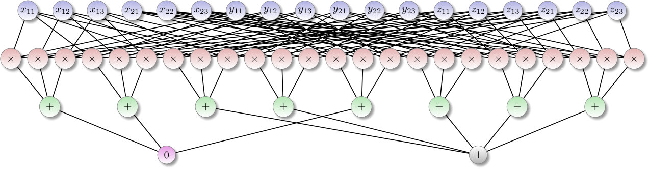 Figure 1
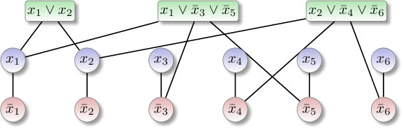 Figure 2
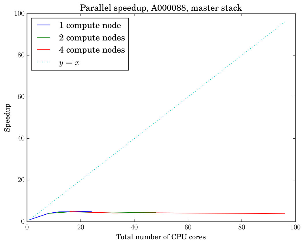 Figure 3
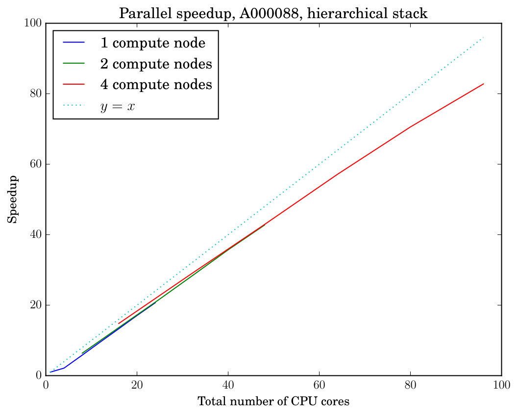 Figure 4
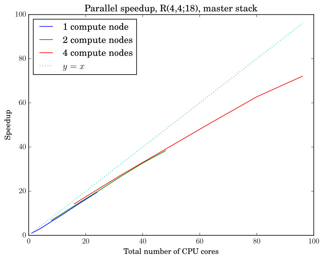 Figure 5
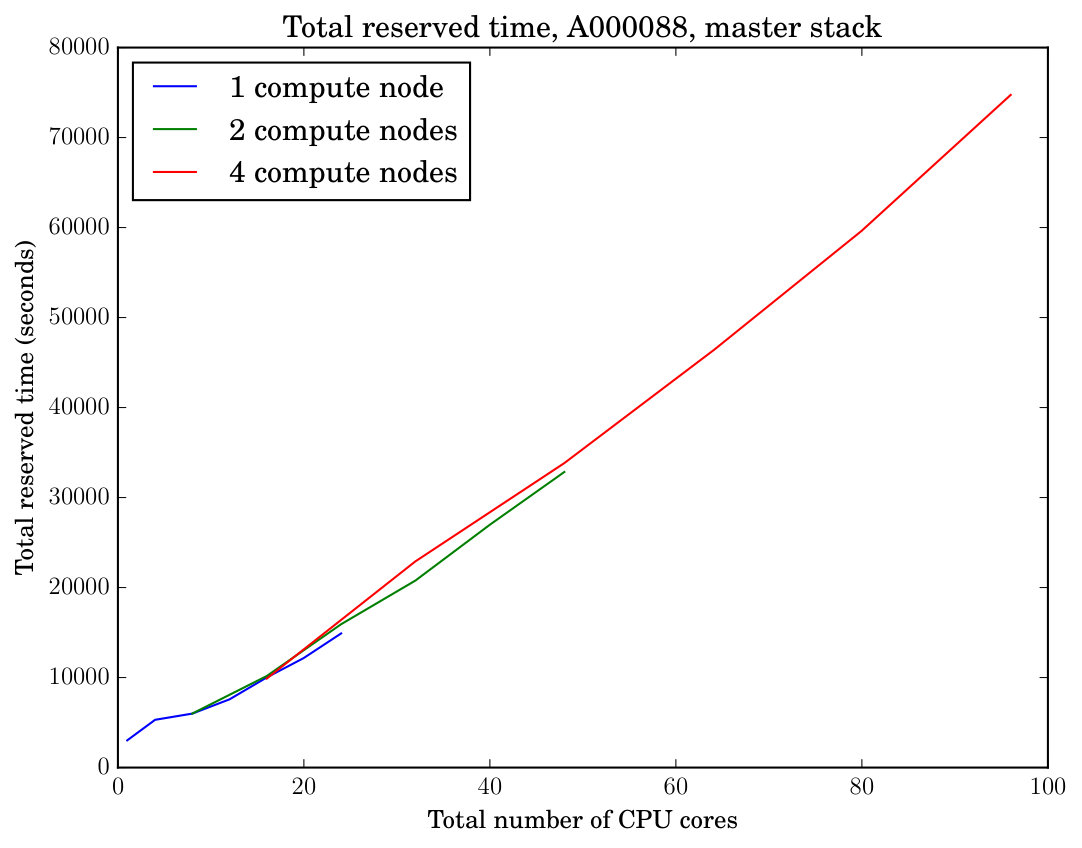 Figure 6
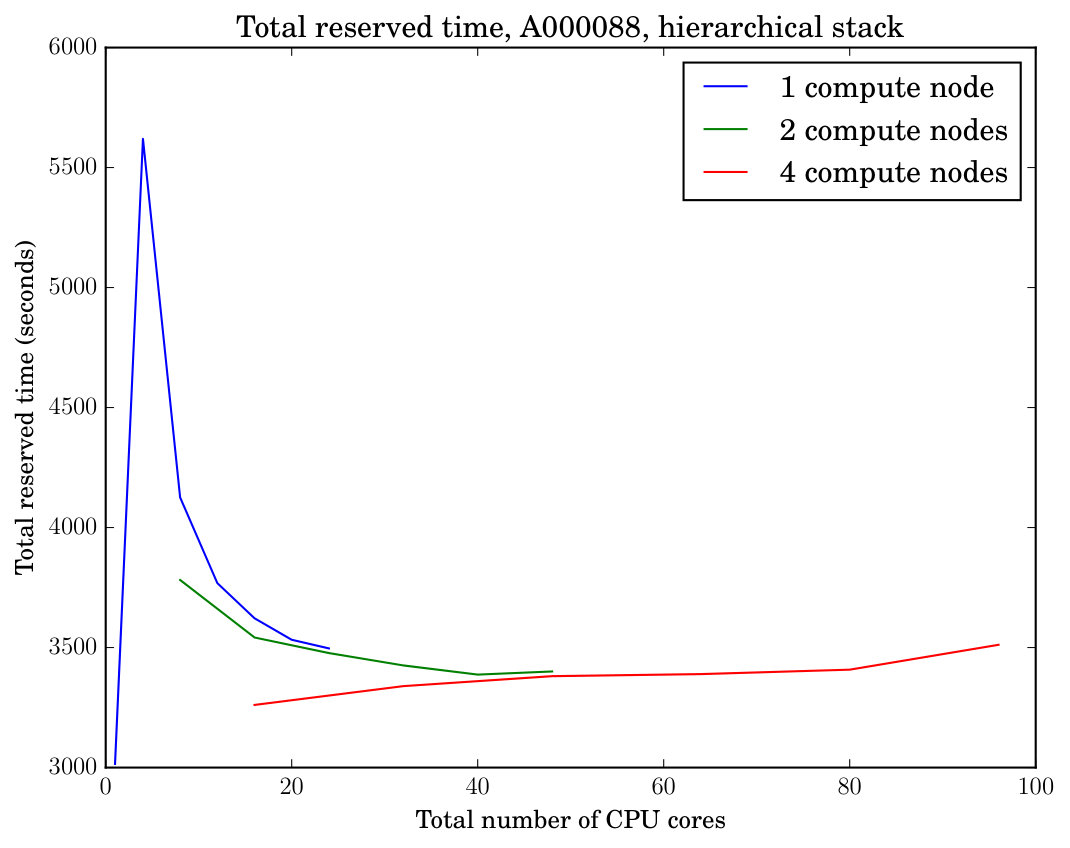 Figure 7
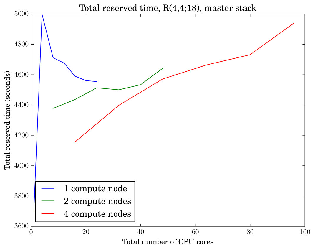 Figure 8
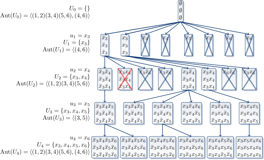 Figure 9
| level | assignments | level | assignments | level | assignments | ||
|---|---|---|---|---|---|---|---|
| 1 | 2 | 12 | 13 | 23 | 1848 | ||
| 2 | 3 | 13 | 14 | 24 | 2400 | ||
| 3 | 4 | 14 | 15 | 25 | 2970 | ||
| 4 | 5 | 15 | 16 | 26 | 3520 | ||
| 5 | 6 | 16 | 17 | 27 | 4004 | ||
| 6 | 7 | 17 | 18 | 28 | 4368 | ||
| 7 | 8 | 18 | 96 | 29 | 4550 | ||
| 8 | 9 | 19 | 300 | 30 | 4480 | ||
| 9 | 10 | 20 | 560 | 31 | 4080 | ||
| 10 | 11 | 21 | 910 | 32 | 3264 | ||
| 11 | 12 | 22 | 1344 | 33 | 1050 |
| level | assignments | level | assignments | level | assignments | ||
|---|---|---|---|---|---|---|---|
| 1 | 2 | 13 | 336 | 25 | 346376 | ||
| 2 | 3 | 14 | 336 | 26 | 47418 | ||
| 3 | 4 | 15 | 140 | 27 | 644016 | ||
| 4 | 5 | 16 | 1216 | 28 | 3256288 | ||
| 5 | 6 | 17 | 5256 | 29 | 4336496 | ||
| 6 | 7 | 18 | 9936 | 30 | 508140 | ||
| 7 | 8 | 19 | 13664 | 31 | 5245032 | ||
| 8 | 9 | 20 | 13104 | 32 | 19768096 | ||
| 9 | 42 | 21 | 2676 | 33 | 2409488 | ||
| 10 | 120 | 22 | 34500 | 34 | 13814848 | ||
| 11 | 200 | 23 | 183120 | 35 | 4147832 | ||
| 12 | 280 | 24 | 328032 | 36 | 274668 |
| with auxiliary graph | ||||||||||||
| raw | prep. | breakid | prep. | reduce | ||||||||
| glucose | lingeling | breakid | glucose | lingeling | reduce | glucose | lingeling | ilingeling | Sat? | |||
| 5 | 7 | 9 | t/o | t/o | 0.28 | 30.07 | 30.73 | 87.35 | 77.87 | 66.40 | 47.67 | No |
| 5 | 8 | 9 | 0.36 | 3.91 | 0.63 | 0.33 | 5.61 | 290.70 | 1.69 | 13.93 | 0.50 | Yes |
| 5 | 8 | 20 | t/o | t/o | 0.61 | 1078.54 | 1273.49 | 290.78 | 2641.97 | 7699.27 | 885.01 | No |
| 5 | 9 | 20 | 1.44 | 1.28 | 1.68 | 72.09 | 26.33 | 881.85 | 228.06 | 371.09 | 40.57 | Yes |
| raw | prep. | breakid | prep. | reduce | |||||||
|---|---|---|---|---|---|---|---|---|---|---|---|
| glucose | lingeling | breakid | glucose | lingeling | reduce | glucose | lingeling | ilingeling | |||
| 15 | 5 | 4 | 722.32 | 811.59 | 2.82 | 126.35 | 154.27 | 19.34 | 19.82 | 31.61 | 32.92 |
| 16 | 5 | 4 | 1038.88 | 1839.05 | 10.68 | 238.52 | 570.19 | 8.07 | 25.62 | 39.55 | 38.31 |
| 17 | 5 | 4 | 4481.54 | 8865.19 | 1.94 | 597.35 | 498.20 | 12.81 | 105.35 | 57.96 | 54.66 |
| 18 | 5 | 4 | 2709.96 | 4762.23 | 9.96 | 559.86 | 460.70 | 14.11 | 40.68 | 74.71 | 66.19 |
| 19 | 5 | 4 | 6701.65 | 6819.77 | 10.66 | 586.81 | 651.10 | 19.13 | 107.73 | 106.62 | 85.38 |
| 20 | 5 | 4 | 8901.20 | 7777.35 | 1.15 | 1294.31 | 1579.77 | 25.37 | 157.91 | 134.55 | 248.56 |
| 12 | 6 | 5 | 38835.75 | 15517.28 | 9.87 | 1602.96 | 745.83 | 2.42 | 1190.58 | 677.38 | 751.27 |
| 13 | 6 | 5 | 26017.87 | 50312.82 | 9.91 | 7032.11 | 3506.61 | 9.68 | 1439.84 | 1440.30 | 1420.10 |
| 14 | 6 | 5 | t/o | t/o | 2.28 | 8417.69 | 5384.79 | 17.18 | 2360.88 | 5559.26 | 2543.99 |
| 15 | 6 | 5 | t/o | t/o | 9.05 | 10537.53 | 7316.61 | 6.49 | 3504.82 | 4104.10 | 4140.57 |
| 16 | 6 | 5 | t/o | t/o | 9.46 | 41355.16 | 27699.48 | 30.52 | 6858.69 | 5612.36 | 5708.18 |
| 17 | 6 | 5 | t/o | t/o | 0.94 | t/o | t/o | 11.48 | 11329.16 | 20597.16 | 10460.73 |
| 18 | 6 | 5 | t/o | t/o | 5.34 | t/o | t/o | 23.81 | 17347.43 | 52703.19 | 16873.36 |
| 19 | 6 | 5 | t/o | t/o | 7.18 | t/o | t/o | 82.93 | 29689.84 | 19969.09 | 21195.04 |
| 20 | 6 | 5 | t/o | t/o | 3.38 | t/o | t/o | 29.36 | 76600.29 | 35850.94 | 27035.80 |
| 21 | 6 | 5 | t/o | t/o | 1.50 | t/o | t/o | 148.64 | t/o | 45963.02 | 48542.48 |
| 22 | 6 | 5 | t/o | t/o | 1.74 | t/o | t/o | 198.15 | t/o | 61414.88 | 66279.68 |
| 23 | 6 | 5 | t/o | t/o | 1.91 | t/o | t/o | 267.67 | t/o | t/o | 78463.34 |
| reduce | ||||
|---|---|---|---|---|
| with | without | |||
| graph | graph | |||
| 15 | 5 | 4 | 19.34 | 399.25 |
| 16 | 5 | 4 | 8.07 | 158.47 |
| 17 | 5 | 4 | 12.81 | 223.24 |
| 18 | 5 | 4 | 14.11 | 1151.05 |
| 19 | 5 | 4 | 19.13 | 1629.34 |
| 20 | 5 | 4 | 25.37 | 586.78 |
| 12 | 6 | 5 | 2.42 | 139.14 |
| 13 | 6 | 5 | 9.68 | 61.46 |
| 14 | 6 | 5 | 17.18 | 381.85 |
| 15 | 6 | 5 | 6.49 | 587.87 |
| 16 | 6 | 5 | 30.52 | 881.09 |
| 17 | 6 | 5 | 11.48 | 322.53 |
| 18 | 6 | 5 | 23.81 | 450.28 |
| 19 | 6 | 5 | 82.93 | 2388.18 |
| 20 | 6 | 5 | 29.36 | 851.68 |
| 21 | 6 | 5 | 148.64 | 1195.23 |
| 22 | 6 | 5 | 198.15 | 1543.51 |
| 23 | 6 | 5 | 267.67 | 5545.20 |
Peer Reviews
No public reviews on file for this paper yet. If you reviewed it on a platform where reviews are public (OpenReview, ICLR, NeurIPS, ICML), you can paste yours below so the community can read it here.
Code & Models
Videos
No videos yet. Explain this paper in a talk, walkthrough, or lecture? Add one.
An adaptive prefix-assignment technique
for symmetry reduction
Tommi Junttila*†*
,
Matti Karppa*†*
,
Petteri Kaski*†*
and
Jukka Kohonen*†‡*
† Aalto University, Department of Computer Science
*‡*Current address: University of Helsinki, Department of Computer Science
Abstract.
This paper presents a technique for symmetry reduction that adaptively assigns a prefix of variables in a system of constraints so that the generated prefix-assignments are pairwise nonisomorphic under the action of the symmetry group of the system. The technique is based on McKay’s canonical extension framework [J. Algorithms 26 (1998), no. 2, 306–324]. Among key features of the technique are (i) adaptability—the prefix sequence can be user-prescribed and truncated for compatibility with the group of symmetries; (ii) parallelizability—prefix-assignments can be processed in parallel independently of each other; (iii) versatility—the method is applicable whenever the group of symmetries can be concisely represented as the automorphism group of a vertex-colored graph; and (iv) implementability—the method can be implemented relying on a canonical labeling map for vertex-colored graphs as the only nontrivial subroutine. To demonstrate the practical applicability of our technique, we have prepared an experimental open-source implementation of the technique and carry out a set of experiments that demonstrate ability to reduce symmetry on hard instances. Furthermore, we demonstrate that the implementation effectively parallelizes to compute clusters with multiple nodes via a message-passing interface.
1. Introduction
1.1. Symmetry reduction
Systems of constraints often have substantial symmetry. For example, consider the following system of Boolean clauses:
[TABLE]
The associative and commutative symmetries of disjunction and conjunction induce symmetries between the variables of (1), a fact that can be captured by stating that the group generated by the two permutations and consists of all permutations of the variables that map (1) to itself. That is, is the automorphism group of the system (1), cf. Section 2.
Known symmetry in a constraint system is a great asset from the perspective of solving the system, in particular since symmetry enables one to disregard partial solutions that are isomorphic to each other under the action of on the space of partial solutions. Techniques for such isomorph rejection111A term introduced by J. D. Swift [64]; cf. Hall and Knuth [32] for a survey on early work on exhaustive computer search and combinatorial analysis. [64] (alternatively, symmetry reduction or symmetry breaking) are essentially mandatory if one desires an exhaustive traversal of the (pairwise nonisomorphic) solutions of a highly symmetric system of constraints, or if the system is otherwise difficult to solve, for example, with many “dead-end” partial solutions compared with the actual number of solutions.
A prerequisite to symmetry reduction is that the symmetries are known. In many cases it is possible to automatically discover and compute these symmetries to enable practical and automatic symmetry reduction. In this context the dominant computational approach for combinatorial systems of constraints is to represent via the automorphism group of a vertex-colored graph that captures the symmetries in the system. Carefully engineered tools for working with symmetries of vertex-colored graphs [20, 40, 51, 53] and permutation group algorithms [15, 61] then enable one to perform symmetry reduction. For example, for purposes of symmetry computations we may represent (1) as the following vertex-colored graph:
[TABLE]
In particular, the graph representation (2) enables us to discover and reduce symmetry to avoid redundant work when solving the underlying system (1).
1.2. Our contribution
The objective of this paper is to present a novel technique for symmetry reduction on systems of constraints. The technique is based on adaptively assigning values to a prefix of the variables so that the obtained prefix-assignments are pairwise nonisomorphic under the action of . The technique can be seen as an instantiation of McKay’s [52] influential canonical extension framework for isomorph-free exhaustive generation.
To give a brief outline of the technique, suppose we are working with a system of constraints over a finite set of variables that take values in a finite set . Suppose furthermore that is the automorphism group of the system. Select distinct variables in . These variables form the prefix sequence considered by the method. The technique works by assigning values in to the variables of the prefix, in prefix-sequence order, with assigned first, then , then , and so forth, so that at each step the partial assignments so obtained are pairwise nonisomorphic under the action of . For example, in (1) the partial assignments and are isomorphic since maps one assignment onto the other; in total there are three nonisomorphic assignments to the prefix in (1), namely (i) , (ii) , and (iii) . Each partial assignment that represents an isomorphism class can then be used to reduce redundant work when solving the underlying system by standard techniques—in the nonincremental case, the system is augmented with a symmetry-breaking predicate requiring that one of the nonisomorphic partial assignments holds, while in the incremental setting [34, 65] the partial assignments can be solved independently or even in parallel.
Our contribution in this paper lies in how the isomorph rejection is implemented at the level of isomorphism classes of partial assignments by careful reduction to McKay’s [52] isomorph-free exhaustive generation framework. The key technical contribution is that we observe how to generate the partial assignments in a normalized form that enables both adaptability (that is, the prefix can be arbitrarily selected to match the structure of ) and precomputation of the extending variable-value orbits along a prefix.
Among further key features of the technique are:
- (1)
Implementability. The technique can be implemented by relying on a canonical labeling map for vertex-colored graphs (cf. [40, 51, 53]) as the only nontrivial subroutine that is invoked once for each partial assignment considered. 2. (2)
Versatility. The method is applicable whenever the group of symmetries can be concisely represented as a vertex-colored graph; cf. (1) and (2). This is useful in particular when the underlying system has symmetries that are not easily discoverable from the final constraint encoding, for example, due to the fact that the constraints have been compiled or optimized222For a beautiful illustration, we refer to Knuth’s [45, §7.1.2, Fig. 10] example of optimum Boolean chains for 5-variable symmetric Boolean functions—from each optimum chain it is far from obvious that the chain represents a symmetric Boolean function. (See also Example 3.) from a higher-level representation in a symmetry-obfuscating manner. A graphical representation can represent such symmetry directly and independently of the compiled/optimized form of the system. 3. (3)
Parallelizability. As a corollary of implementing McKay’s [52] framework, the technique does not need to store representatives of isomorphism classes in memory to perform isomorph rejection, which enables easy parallelization since the partial assignments can be processed independently of each other.
The required mathematical preliminaries on symmetry and McKay’s framework are reviewed in Sections 2 and 3, respectively. The main technical contribution of this paper is developed in Section 4 where we present the prefix-assignment technique that we will subsequently extend to account for value symmetry in Section 5. Our development in Sections 4 and 5 relies on an abstract group , with the understanding that a concrete implementation can be designed e.g. in terms of a vertex-colored graph representation, as will be explored in Section 6.
To demonstrate the practical applicability of our technique, we have prepared an open-source parallel implementation [41]. The implementation is structured as a preprocessor that works with an explicitly given graph representation and utilizes the nauty [51, 53] canonical labeling software for vertex-colored graphs as a subroutine to prepare an exhaustive collection of nonisomorphic prefix assignments relative to a user-supplied prefix of variables, and the Message Passing Interface (MPI) for parallelization. Further details of the implementation are presented in Section 7. In Section 8, we report on a set of experiments that (i) demonstrate the ability to reduce symmetry on hard instances, (ii) study the serendipity of an auxiliary graph for encoding the symmetries in an instance, (iii) give examples of instances with hard combinatorial symmetry where our technique performs favorably in comparison with earlier techniques, and (iv) study the parallel speedup obtainable when we distribute the symmetry reduction task to a compute cluster with multiple compute nodes.
1.3. Earlier work
A classical way to exploit symmetry in a system of constraints is to augment the system with so-called symmetry-breaking predicates (SBP) that eliminate either some or all symmetric solutions [5, 19, 28, 59]. Such constraints are typically lexicographic leader (lex-leader) constraints that are derived from a generating set for the group of symmetries . Among recent work in this area, Devriendt et al. [22] extend the approach by presenting a more compact way for expressing SBPs and a method for detecting “row interchangeabilities”. Itzhakov and Codish [39] present a method for finding a set of symmetries whose corresponding lex-leader constraints are enough to completely break symmetries in search problems on small (10-vertex) graphs; this approach is extended by Codish et al. [17] by adding pruning predicates that simulate the first iterations of the equitable partition refinement algorithm of nauty [51, 53]. Heule [35] shows that small complete symmetry-breaking predicates can be computed by considering arbitrary Boolean formulas instead of lex-leader formulas.
Our present technique can be seen as a method for producing symmetry-breaking predicates by augmenting the system of constraints with the disjunction of the nonisomorphic partial assignments. The main difference to the related work above is that our technique does not produce the symmetry-breaking predicate from a set of generators for but rather the predicate is produced recursively, and with the possibility for parallelization, by classifying orbit representatives up to isomorphism using McKay’s [52] framework. As such our technique breaks all symmetry with respect to the prescribed prefix, but comes at the cost of additional invocations of graph-automorphism and canonical-labeling tools. This overhead and increased symmetry reduction in particular means that our technique is best suited for constraint systems with hard combinatorial symmetry that is not easily capturable from a set of generators, such as symmetry in combinatorial classification problems [42]. In addition to McKay’s [52] canonical extension framework, other standard frameworks for isomorph-free exhaustive generation in this context include orderly algorithms due to Faradžev [26] and Read [57], as well as the homomorphism principle for group actions due to Kerber and Laue [44].
It is also possible to break symmetry within a constraint solver during the search by dynamically adding constraints that rule out symmetric parts of the search space (cf. [16, 28]). If we use the nonisomorphic partial assignments produced by our technique as assumption sequences (cubes) in the incremental cube-and-conquer approach [34, 65], our technique can be seen as a restricted way of breaking the symmetries in the beginning of the search, with the benefit—as with cube-and-conquer—that the portions of the search space induced by the partial assignments can be solved in parallel, either with complete independence or with appropriate sharing of information (such as conflict clauses) between the parallel nodes executing the search. For further work in dynamic symmetry breaking, cf. [21, 10, 8, 58, 60, 9, 23].
For work on isomorphism and canonical labeling techniques, cf. [7, 30, 49, 53].
2. Preliminaries on group actions and symmetry
This section reviews relevant mathematical preliminaries and notational conventions for groups, group actions, symmetry, and isomorphism for our subsequent development. (Cf. [15, 25, 38, 42, 43, 61] for further reference.)
2.1. Groups and group actions
Let be a finite group and let be a finite set (the domain) on which acts. For two groups and , let us write to indicate that is a subgroup of . We use exponential notation for group actions, and accordingly our groups act from the right. That is, for an object and , let us write for the object in obtained by acting on with . Accordingly, we have for all and . For a finite set , let us write for the group of all permutations of with composition of mappings as the group operation.
2.2. Orbit and stabilizer, the automorphism group
For an object let us write for the orbit of under the action of and for the stabilizer subgroup of in . Equivalently we say that is the automorphism group of and write whenever is clear from the context; if we want to stress the acting group we write .
We write for the set of all orbits of on . For and , let us write for the -conjugate of . For all and we have . That is, the automorphism groups of objects in an orbit are conjugates of each other.
2.3. Isomorphism
We say that two objects are isomorphic if they are on the same orbit of in . In particular, are isomorphic if and only if there exists an isomorphism from to that satisfies . An isomorphism from an object to itself is an automorphism. Let us write for the set of all isomorphisms from to . We have that where is arbitrary. Let us write to indicate that and are isomorphic. If we want to stress the group under whose action isomorphism holds, we write .
2.4. Elementwise action on tuples and sets
Suppose that acts on two sets, and . We extend the action to the Cartesian product elementwise by defining for all and . Isomorphism extends accordingly; for example, we say that and are isomorphic and write if there exists a with and . Suppose that acts on a set . We extend the action of on to an elementwise action of on subsets by setting for all and . In what follows we will tacitly work with these elementwise actions on tuples and sets unless explicitly otherwise indicated.
2.5. Canonical labeling and canonical form
A function is a canonical labeling map for the action of on if
[TABLE]
For we say that is the canonical form of in . From (K) it follows that isomorphic objects have identical canonical forms, and the canonical labeling map gives an isomorphism that takes an object to its canonical form.
We assume that the act of computing for a given produces as a side-effect a set of generators for the automorphism group .
3. McKay’s canonical extension method
This section reviews McKay’s [52] canonical extension method for isomorph-free exhaustive generation. Mathematically it will be convenient to present the method so that the isomorphism classes are captured as orbits of a group action of a group , and extension takes place in one step from “seeds” to “objects” being generated, with the understanding that the method can be applied inductively in multiple steps so that the “objects” of the current step become the “seeds” for the next step. For completeness and ease of exposition, we also give a correctness proof for the method. We stress that all material in this section is well known. (Cf. [42].)
3.1. Objects and seeds
Let be a finite set of objects and let be a finite set of seeds. Let be a finite group that acts on and . Let be a canonical labeling map for the action of on .
3.2. Extending seeds to objects.
Let us connect the objects and the seeds by means of a relation that indicates which objects can be built from which seeds by extension. For and we say that extends and write if . We assume the relation satisfies
[TABLE]
For a seed , let us write for the set of all objects that extend .
3.3. Canonical extension
We associate with each object a particular isomorphism-invariant extension by which we want to extend the object from a seed. A function is a canonical extension map if
[TABLE]
That is, (M1) requires that is in fact an extension of and (M2) requires that isomorphic objects have isomorphic canonical extensions. In particular, is a well-defined map from to .
3.4. Generating objects from seeds
Let us study the following procedure, which is invoked for exactly one representative from each orbit in :
[TABLE]
Let us first consider the case when there are no isomorph rejection tests.
Lemma 1**.**
The procedure (P) visits every isomorphism class of objects in at least once.
Proof.
To see that every isomorphism class is visited, let be arbitrary. By (E2), there exists a with . By our assumption on how procedure (P) is invoked, is isomorphic to a unique such that procedure (P) is invoked with input . Let be an associated isomorphism with . By (E1) and , we have for . By the structure of procedure (P) we observe that is visited and . Since was arbitrary, all isomorphism classes are visited at least once. ∎
Let us next modify procedure (P) so that any two visits to the same isomorphism class of objects originate from the same procedure invocation. Let be a canonical extension map. Whenever we construct by extending in procedure (P), let us visit if and only if
[TABLE]
Lemma 2**.**
The procedure (P) equipped with the test (T1) visits every isomorphism class of objects in at least once. Furthermore, any two visits to the same isomorphism class must (i) originate by extension from the same procedure invocation on input , and (ii) belong to the same -orbit of this seed .
Proof.
Suppose that is visited by extending and is visited by extending , with . By (T1) we must thus have and . Furthemore, from (M2) we have . Thus, and hence . Since , we must in fact have by our assumption on how procedure (P) is invoked. Since and were arbitrary, any two visits to the same isomorphism class must originate by extension from the same seed. Furthermore, we have and thus . Let us next observe that every isomorphism class of objects is visited at least once. Indeed, let be arbitrary. By (M1), we have . In particular, there is a unique with such that procedure (P) is invoked with input . Let be an associated isomorphism with . By (E1), we have for . Furthermore, implies by (M2) that , so (T1) holds and is visited. Since and was arbitrary, every isomorphism class is visited at least once. ∎
Let us next observe that the outcome of test (T1) is invariant on each -orbit of extensions of .
Lemma 3**.**
For all we have that (T1) holds for if and only if (T1) holds for .
Proof.
From and (M2) we have . Thus, if and only if . ∎
Lemma 3 in particular implies that we obtain complete isomorph rejection by combining the test (T1) with a further test that ensures complete isomorph rejection on -orbits. Towards this end, let us associate an arbitrary order relation on every -orbit on . Let us perform the following further test:
[TABLE]
The following lemma is immediate from Lemma 2 and Lemma 3.
Lemma 4**.**
The procedure (P) equipped with the tests (T1) and (T2) visits every isomorphism class of objects in exactly once.
3.5. A template for canonical extension maps
We conclude this section by describing a template of how to use an arbitrary canonical labeling map to construct a canonical extension map .
For construct the canonical form . Using the canonical form only, identify a seed with . In particular, such a seed must exist by (E2). (Typically this identification can be carried out by studying and finding an appropriate substructure in that qualifies as . For example, may be the minimum seed in that satisfies . Cf. Lemma 9.) Once has been identified, set .
Lemma 5**.**
The map above is a canonical extension map.
Proof.
By (E1) we have because , , and . Thus, (M1) holds for . To verify (M2), let with be arbitrary. Since , by (K) we have . It follows that and , implying that is an isomorphism witnessing . Thus, (M2) holds for . ∎
4. Generation of partial assignments via a prefix sequence
This section describes an instantiation of McKay’s method that generates partial assignments of values to a set of variables one variable at a time following a prefix sequence at the level of isomorphism classes given by the action of a group on . We postpone the extension to include variables to Section 5. Let be a finite set where the variables in take values.
4.1. Partial assignments, isomorphism, restriction
For a subset of variables, let us say that a partial assignment of values to is a mapping . Isomorphism for partial assignments is induced by the following group action. Let act on by setting where is defined for all by
[TABLE]
Lemma 6**.**
The action (3) is well-defined.
Proof.
We observe that for the identity of we have . Furthermore, for all and we have
[TABLE]
For an assignment , let us write for the underlying set of variables assigned by . Observe that the underline map is a homomorphism of group actions in the sense that
[TABLE]
holds for all and . For , let us write for the restriction of to .
4.2. The prefix sequence and generation of normalized assignments
We are now ready to describe the generation procedure. Let us begin by prescribing the prefix sequence. Let be distinct elements of and let for . In particular we observe that
[TABLE]
with for all .
For let consist of all partial assignments with . Or what is the same, using the underline notation, consists of all partial assignments with .
We rely on canonical extension to construct exactly one object from each orbit of on , using as seeds exactly one object from each orbit of on , for each . We assume the availability of canonical labeling maps for each .
Our construction procedure will work with objects that are in a normal form to enable precomputation for efficient execution of the subsequent tests for isomorph rejection. Towards this end, let us say that is normalized if . It is immediate from our definition of and (3) that each orbit in contains at least one normalized object.
Let us begin with a high-level description of the construction procedure, to be followed by the details of the isomorph rejection tests and a proof of correctness. Fix and study the following procedure, which we assume is invoked for exactly one normalized representative from each orbit in :
[TABLE]
From an implementation point of view, it is convenient to precompute the orbit together with group elements for each that satisfy . Indeed, a constructed with can now be normalized by acting with on to obtain a normalized isomorphic to .
4.3. The isomorph rejection tests
Let us now complete the description of procedure (P’) by describing the two isomorph rejection tests (T1’) and (T2’). This subsection only describes the tests with an implementation in mind, the correctness analysis is postponed to the following subsection.
Let us assume that the elements of have been arbitrarily ordered and that is a canonical labeling map. Suppose that has been constructed by extending a normalized with . The first test is:
[TABLE]
From an implementation perspective we observe that we can precompute the orbit . Furthermore, the only computationally nontrivial part of the test is the computation of since we assume that we obtain generators for as a side-effect of this computation. Indeed, with generators for available, it is easy to compute the orbits and hence to test whether .
Let us now describe the second test:
[TABLE]
From an implementation perspective we observe that since is normalized we have and thus the orbit considered by procedure (P’) partitions into one or more -orbits. Furthermore, generators for are readily available (due to itself getting accepted in the test (T1’) at an earlier level of recursion), and thus the orbits and their minimum elements are cheap to compute. Thus, a fast implementation of procedure (P’) will in most cases execute the test (T2’) before the more expensive test (T1’).
Example 1*.*
We display below a possible search tree for the system of clauses (1) and the prefix sequence . Each node in the search tree displays the prefix assignment (top), its canonical version (middle) and its normalized version (bottom). The variables have the Boolean domain and the assignments are given in the literal form; for example, we write for the assignment .
The nodes with a red cross are nodes eliminated by the test (T1’) and the ones with a blue cross are eliminated by the test (T2’). (For convenience of display, these eliminated nodes are only drawn in the first three levels above.) For instance, the node with is eliminated by the test (T1’) because the minimum such that when and is and as . On the other hand, the node with is eliminated by the test (T2’) as and . We observe that the search tree has dead-end nodes that do not extend to any full prefix assignment.
4.4. Correctness
We now establish the correctness of procedure (P’) together with the tests (T1’) and (T2’) by reduction to McKay’s framework and Lemma 4. Fix . Let us start by defining the extension relation for all and by setting if and only if
[TABLE]
This relation is well-defined in the context of McKay’s framework:
Lemma 7**.**
The relation (5) satisfies (E1) and (E2).
Proof.
To establish (E1), let and be arbitrary. It suffices to show that for all we have if and only if . Let be arbitrary. By (4), for all we have if and only if . Similarly, for any we have if and only if . Finally, for any that satisfies and (equivalently, satisfies and ), we have if and only if . To establish (E2), observe that for an arbitrary there exists a with , and thus holds for , where is obtained from by deleting the assignment to the variable . ∎
The following lemma establishes that the iteration in procedure (P’) constructs exactly the objects ; cf. procedure (P).
Lemma 8**.**
Let be normalized. For all we have if and only if there exists a with and .
Proof.
From (5) we have that if and only if there exists a with , , and . Since is normalized, we have and hence . Thus, and
[TABLE]
Thus, to establish the “only if” direction of the lemma, take , and for the “if” direction, take with . ∎
Next we show the correctness of the test (T1’) by establishing that it is equivalent with the test (T1) for a specific canonical extension function . Towards this end, let us use the assumed canonical labeling map to build a canonical extension function using the template of Lemma 5. In particular, given an as input with , first construct the canonical form . In accordance with (T1’), select the minimum such that . Now construct from by deleting the value of .
Lemma 9**.**
The mapping is well-defined and satisfies both (M1) and (M2).
Proof.
From (4) we have both and . Thus,
[TABLE]
It follows that the choice of depends on and but not on the choices of or . Furthermore, we observe that and . Thus, the construction of is well-defined and (M2) holds by Lemma 5.
To verify (M1), observe that since , there exists an with . Thus, for we have , , and . Thus, from (5) we have and thus (M1) holds. ∎
To complete the equivalence between (T1’) and (T1), observe that since and determine by , and similarly and determine by , the test (T1) is equivalent to testing whether holds, that is, whether holds. Observe that this is exactly the test (T1’).
It remains to establish the equivalence of (T2’) and (T2). We start with a lemma that captures the -orbits considered by (T2).
Lemma 10**.**
For a normalized the orbits in are in a one-to-one correspondence with the elements of .
Proof.
From (3) we have since is normalized. Furthermore, Lemma 8 implies that every extension is uniquely determined by the variable and the value . Since the action (3) fixes the values in elementwise, for any we have if and only if both and . The lemma follows. ∎
Now order the elements based on the lexicographic ordering of the pairs . Since the action (3) fixes the values in elementwise, we have that (T2’) holds if and only if (T2) holds for this ordering of . The correctness of procedure (P’) equipped with the tests (T1’) and (T2’) now follows from Lemma 4.
4.5. Selecting a prefix
This section gives a brief discussion on how to select the prefix. Let be the set of variables in the prefix sequence. It is immediate that there exist distinct partial assignments from to . Let us write for the set of these assignments. The group now partitions into orbits via the action (3), and it suffices to consider at most one representative from each orbit to obtain an exhaustive traversal of the search space, up to isomorphism. Our goal is thus to select the prefix so that the setwise stabilizer has comparatively few orbits on compared with the total number of such assignments. In particular, the ratio of the number of orbits to the total number of mappings can be viewed as a proxy for the achieved symmetry reduction and as a rough333Here it should be noted that executing the symmetry reduction carries in itself a nontrivial computational cost. That is, there is a tradeoff between the potential savings in solving the system gained by symmetry reduction versus the cost of performing symmetry reduction. For example, if the instance has no symmetry and is a trivial group, then executing symmetry reduction merely makes it more costly to solve the system. proxy for the speedup factor obtained compared with no symmetry reduction at all.
4.6. Subroutines
By our assumption, the canonical labeling map produces as a side-effect a set of generators for the automorphism group for a given input . We also assume that generators for the groups for can be precomputed by similar means. This makes the canonical labeling map essentially the only nontrivial subroutine needed to implement procedure (P’). Indeed, the orbit computations required by tests (T1’) and (T2’) are implementable by elementary permutation group algorithms [15, 61]. Section 6 describes how to implement by reduction to vertex-colored graphs.444Reduction to vertex-colored graphs is by no means the only possibility to obtain the canonical labeling map to enable (P’), (T1’), and (T2’). Another possibility would be to represent directly as a permutation group and use dedicated permutation-group algorithms [47, 48]. Our present choice of vertex-colored graphs is motivated by easy availability of carefully engineered implementations for working with vertex-colored graphs.
5. Value symmetries
The previous section considered prefix-assignment generation subject to an action of a group on the set of variables . In this section, we extend the framework so that it captures symmetries in values assigned to variables, or value symmetries. Towards this end, we extend the domain that records the symmetries from to , where is the set of values that can be assigned to the variables in . Accordingly, in what follows we assume that the group acts on as well as on , the latter by restriction.
The action of the group on may not be completely arbitrary, however, because we want partial assignments with to remain well-defined functions under the action of . This property is naturally captured by the wreath product group and its natural action on .
5.1. The wreath product and its actions
We will follow the convention that acts on by first acting on and then on . For accessibility and convenience, we review our conventions in detail. The group consists of all pairs , where is a permutation of and associates a permutation with each element . In particular, has order .
The product of two elements is defined by , where
[TABLE]
and for all we set
[TABLE]
The inverse of an element is thus given by , where
[TABLE]
and for all we have
[TABLE]
An element acts on an element by
[TABLE]
and on a pair by
[TABLE]
Here in particular the intuition is that we first act on with to obtain , and then act with to obtain . Extend the action (11) elementwise to subsets .
5.2. Partial assignments and isomorphism
Let be a subgroup of and let act on and by (11) and (12), respectively. Furthermore, we let an element act on a partial assignment with to produce the partial assignment defined for all by
[TABLE]
In analogy with Lemma 6, let us verify that the value-permuting action (13) is well-defined.
Lemma 11**.**
The action (13) is well defined.
Proof.
We observe that for the identity of , we have . Furthermore, for all , , and , by (13), (7), and (8), we have
[TABLE]
Let us recall that for we write for the underlying set of variables assigned by . In analogy with Section 4.1, the underline map is a homomorphism of group actions that satisfies (4) for the action (13) and the action (11) extended elementwise to subsets of . Isomorphism for partial assignments is now induced by the action (13).
5.3. Generating normalized assignments
Working with the group action (13), let be distinct elements of , and let for . Let consist of all partial assignments with . We construct exactly one object form each orbit of on , using as seeds exactly one object from each orbit of on , for each , assuming the availability of canonical labeling maps . We say the assignment is normalized if .
We now present a version of the procedure (P’) modified for the group action (13). Let us fix . We assume that the procedure is invoked for exactly one normalized representative from each orbit in .
[TABLE]
In particular, procedure (P”) has two differences compared with procedure (P’). First, the underlying group action is (13). Second, the test (T2’) has been replaced with a new test (T2”) to account for more extensive orbits of pairs under the action of .
5.4. The isomorph rejection tests
Assume that the elements of , , and have been arbitrarily ordered and that is a canonical labeling map. Suppose that has been constructed by extending a normalized with and . Let us first recall the test (T1’) for convenience:
[TABLE]
The new isomorph rejection test is as follows:
[TABLE]
5.5. Correctness
We now establish the correctness of the modified procedure (P”). Fix . Define the extension relation as in (5). This relation is well-defined in the context of McKay’s framework under the modified group action.
Lemma 12**.**
The relation (5) satisfies (E1) and (E2) when the group action is as defined in (13).
Proof.
Identical to Lemma 7 since (4) holds for the action (13) and the action (11) extended elementwise to subsets of . ∎
The correctness analysis of the test (T1’) proceeds identically as in Section 4.1, relying on (4) in the proof of Lemma 9. To establish the correctness of the new test (T2”), we first observe that the counterpart of Lemma 8 holds for the modified group action.
Lemma 13**.**
Let be normalized. For all , we have if and only if there exists a with and .
Proof.
First observe that (6) holds for the action (13). Then proceed as in the proof of Lemma 8. ∎
Let us now proceed to the counterpart of Lemma 10.
Lemma 14**.**
For a normalized , the orbits in are in a one-to-one correspondence with the orbits in .
Proof.
Lemma 13 implies that every extension is uniquely determined by the variable and the value . That is, the elements in are in one-to-one correspondence with elements in .
Let act on via (13); this action is well-defined by Lemma 12 and (E1) since for all we have if and only if . Let act on via (12); this action is well-defined because is normalized and hence holds by (4).
Let be arbitrary with and . We now claim that holds under the action (13) if and only if holds under the action (12). To see this, first observe that for all we have by (4) since is normalized. Furthermore, . Thus, by (13) it holds that for all with and we have if and only if and . Or what is the same by (12), if and only if . ∎
Order the elements based on the lexicographic ordering of the pairs . We now have that (T2”) holds if and only if (T2) holds for this ordering of . The correctness of procedure (P”) equipped with the tests (T1’) and (T2”) now follows from Lemma 4.
6. Representation using vertex-colored graphs
This section describes one possible approach to represent the group of symmetries of a system of constraints over a finite set of variables taking values in a finite set . Our representation of choice will be vertex-colored graphs over a fixed finite set of vertices . In particular, isomorphisms between such graphs are permutations that map edges onto edges and respect the colors of the vertices; that is, every vertex in maps to a vertex of the same color under . It will be convenient to develop the relevant graph representations in steps, starting with the representation of the constraint system and then proceeding to the representation of setwise stabilizers and partial assignments. These representations are folklore (see e.g. [42]) and are presented here for completeness of exposition only.
6.1. Representing the constraint system
To capture via a vertex-colored graph with vertex set , it is convenient to represent the variables directly as a subset of vertices such that no vertex in has a color that agrees with a color of a vertex in . We then seek a graph such that projected to is exactly . In most cases such a graph is concisely obtainable by encoding the system of constraints with additional vertices and edges joined to the vertices representing the variables in . We discuss two examples.
Example 2*.*
Consider the system of clauses (1) and its graph representation (2). The latter can be obtained as follows. First, introduce a blue vertex for each of the six variables of (1). These blue vertices constitute the subset . Then, to accommodate negative literals, introduce a red vertex joined by an edge to the corresponding blue vertex representing the positive literal. These edges between red and blue vertices ensure that positive and negative literals remain consistent under isomorphism. Finally, introduce a green vertex for each clause of (1) with edges joining the clause with each of its literals. It is immediate that we can reconstruct (1) from (2) up to labeling of the variables even after arbitrary color-preserving permutation of the vertices of (2). Thus, (2) represents the symmetries of (1).
Let us next discuss an example where it is convenient to represent the symmetry at the level of original constraints rather than at the level of clauses.
Example 3*.*
Consider the following system of eight cubic equations over 24 variables taking values modulo 2:
[TABLE]
This system seeks to decompose a tensor (whose elements appear on the right hand sides of the equations) into a sum of three rank-one tensors. The symmetries of addition and multiplication modulo 2 imply that the symmetries of the system can be represented by the following vertex-colored graph:
Indeed, we encode each monomial in the system with a product-vertex, and group these product-vertices together by adjacency to a sum-vertex to represent each equation, taking care to introduce two uniquely colored constant-vertices to represent the right-hand side of each equation.
Remark. The representation built directly from the system of polynomial equations in Example 3 concisely captures the symmetries in the system independently of the final encoding of the system (e.g. as CNF) for solving purposes. In particular, building the graph representation from such a final CNF encoding (cf. Example 2) results in a less compact graph representation and obfuscates the symmetries of the original system, implying less efficient symmetry reduction.
6.2. Representing the values
In what follows it will be convenient to assume that the graph contains a uniquely colored vertex for each value in . (Cf. the graph in Example 3.) That is, we assume that and that projected to is the trivial group.
6.3. Representing setwise stabilizers in the prefix chain
To enable procedure (P’) and the tests (T1’) and (T2’), we require generators for for each . More generally, given a subset , we seek to compute a set of generators for the setwise stabilizer , with . Assuming we have available a vertex-colored graph that represents by projection of to , let us define the graph by selecting one vertex and joining each vertex with an edge to the vertex . It is immediate that projected to is precisely .
6.4. Representing partial assignments
Let be an assignment of values in to variables in . Again to enable procedure (P’) together with the tests (T1’) and (T2’), we require a canonical labeling and generators for the automorphism group . Again assuming we have a vertex-colored graph that represents , let us define the graph by joining each vertex with an edge to the vertex . It is immediate that projected to is precisely . Furthermore, a canonical labeling can be recovered from and the canonical form .
6.5. Using tools for vertex-colored graphs
Given a vertex-colored graph as input, practical tools exist for computing a canonical labeling and a set of generators for . Such tools include bliss [40], nauty [51, 53], and traces [53]. Once the canonical labeling and generators are available in it is easy to map back to by projection to so that corresponding elements of are obtained.
7. Parallel implementation
This section outlines the parallel implementation of our technique into a tool called reduce. The implementation is written in C++ and structured as a preprocessor that works with an explicitly given graph representation. In the absence of such an input graph, the graph is constructed automatically from CNF as described in Section 6. The nauty [51, 53] canonical labeling software for vertex-colored graphs is utilized as a subroutine.
7.1. Backtracking search for partial assignments
The backtracking search for partial assignments is implemented using a stack that stores nodes of the search tree. (Recall Example 1 for an illustration of a search tree.) Each node in the stack represents the complete subtree of the search tree rooted at . Initially, the stack consists of the empty assignment, which represents the entire search tree.
Throughout the search, we maintain the invariant that the nodes stored in the stack represent pairwise node-disjoint subtrees of the search tree, which enables us to work through the contents of the stack in arbitrary order and to distribute the contents of the stack to multiple compute nodes as necessary; we postpone a detailed discussion of the distribution of the stack and parallelization of the search to Section 7.2.
Viewed as a sequential process, the search proceeds by iterating the following work procedure until the stack is empty:
[TABLE]
We observe that the procedure (W) above implements procedure (P’) using the stack to maintain the state of the search. In particular, when a single worker process executes the search, we obtain a standard depth-first traversal of the search tree. However, we also observe that procedure (W) pushes all the child nodes of to the stack before consulting the stack for further work. This enables multiple worker processes, all executing procedure (W), to work in parallel, if we take care to ensure that (i) push and pop operations to the stack are atomic, and (ii) the termination condition is changed from the stack being empty to the stack being empty and all worker procedures being idle. Furthermore, as presented in more detail in what follows, we can distribute the stack across multiple compute nodes by appropriately communicating push and pop requests between nodes.
7.2. Parallelization and distributing the stack
We parallelize the search using the OpenMPI implementation [27] of the Message Passing Interface (MPI) [54, 55, 31]. We provide two different communication modes, both of which rely on a master–slave paradigm with processes. The master process with rank 0 distributes the work to worker processes that, in turn, communicate their results back to the master process. We now proceed with a more detailed description of the two communication modes.
Master stack mode. In the simpler of the two modes, the master process stores the entire stack. The worker processes interact with the master directly, making push and pop requests to the master process via MPI messages. While inefficient in terms of communication and in terms of potentially overwhelming the master node, this mode provides load balancing that is empirically adequate for a small number of compute nodes and instances whose search tree is not too wide.
Hierarchical stack mode. The hierarchical stack mode divides the worker nodes into classes, each of which is associated with a subset of levels of the search tree. Each worker process maintains a local stack for nodes at their respective levels. Whenever a worker process pushes an assignment, the assignment is stored in the local stack if the level of the assignment belongs to the levels associated with the node; otherwise, the assignment is communicated to the master process which then pushes the assignment to the global stack maintained in the master process. Whenever a worker process pops an assignment, the worker process first consults its local stack and pops the assignment from the local stack if an assignment is available; otherwise, the worker process makes a pop request to the master process, which supplies an assignment from the global stack as soon as an assignment of one of the levels associated with the worker becomes available. This strategy helps in cases where the search tree becomes very wide; in our experiments, we found that a simple thresholding into one low-level process that processes levels , and high level processes that process levels was sufficient.
For both modes of communication, the master process keeps track of the worker processes that are idle, that is, workers that have sent pop requests that have not been serviced. If all workers are idle and the global stack is empty, the master process instructs all worker processes to exit and then exits itself.
These communication modes serve as a proof-of-concept of the practical parallelizability of our present technique for symmetry reduction. For parallelization to very large compute clusters, we expect that more advanced communication strategies will be required (see, for example, [24, 56] or [55]); however, the implementation of such strategies is beyond the scope of the present work.
8. Experiments
This section documents an experimental evaluation of our parallel implementation of the adaptive prefix-assignment technique. Our main objective is to demonstrate the effective parallelizability of the approach, but we will also report on experiments comparing the performance of our tool (without parallelization) with existing tools that do not parallelize.
8.1. Instances
Let us start by defining the families of input instances used in our experiments. First, we study the usefulness of an auxiliary symmetry graph with systems of polynomial equations aimed at discovering the tensor rank of a small tensor modulo 2, with and . Computing the rank of a given tensor is NP-hard [33].555Yet considerable interest exists to determine tensor ranks of small tensors, in particular tensors that encode and enable fast matrix multiplication algorithms; cf. [1, 2, 3, 4, 13, 14, 18, 36, 46, 63, 66]. For numerical work on discovering small low-rank tensor decompositions, cf. [11, 37, 62]. In precise terms, we seek to find the minimum such that there exist three matrices such that for all we have
[TABLE]
Such instances are easily compilable into CNF with constituting three matrices of Boolean variables so that the task becomes to find the minimum such that the compiled CNF instance is satisfiable. Independently of the target tensor , such instances have a symmetry group of order at least due to the fact that the columns of the matrices can be arbitrarily permuted so that (14) maps to itself. In our experiments, we select the entries of uniformly at random so that the number of s in is exactly . We use the first three rows of the matrix A as the prefix sequence.
As a further family of instances with considerable symmetry, we study the Clique Coloring Problem (CCP) that yields empirically difficult-to-solve instances for contemporary SAT solvers [50]. For positive integer parameters , , and , the CCP asks whether there exists an undirected -colorable graph on nodes such that the graph contains a complete graph as a subgraph. Such instances are unsatisfiable if . The particular encoding that we use (see [50]) is as follows. Introduce variables for with to indicate the presence of an edge joining vertex and , variables for with to indicate that vertex occupies slot in a clique, and variables for and to indicate that vertex has color . The clauses are
- (1)
, 2. (2)
, 3. (3)
, 4. (4)
, and 5. (5)
.
We consider unsatisfiable instances with parameters , , and let vary from 15 to 20 in the case of and 12 to 24 when . We use the variables as the prefix sequence. The auxiliary graph for encoding the symmetries is constructed as follows. Introduce a vertex for each variable , for each variable , and for each variable . These vertices are colored with three distinct colors, one color for each type of variable. Next, introduce three types of auxiliary vertices, with each type colored with its own distinct color. Introduce vertices for the nodes, vertices for the clique slots, and vertices for the node colors. Thus, in total the graph consists of vertices colored with six distinct colors. To complete the construction of the auxiliary graph, introduce edges to the graph so that each variable is joined to the nodes and , each variable is joined to clique slot and to the node , and each variable is joined to the node and to the node color .
We study the parallelizability of our algorithm using two input instances with hard combinatorial symmetry. The first instance, which we call in what follows, is an unsatisfiable CNF instance that asks whether there exists an 18-node graph with the property that neither the graph nor its complement contains the complete graph as a subgraph. That is, we ask whether the Ramsey number satisfies (in fact, [29]). No auxiliary graph is provided to accompany this instance. The second instance consists of an empty CNF over 36 variables together with an auxiliary graph that encodes the isomorphism classes of 9-node graphs by inserting a variable vertex in the middle of each of the edges of the complete graph . Applying reduce with a length-36 prefix sequence (listing the 36 variable vertices in any order) yields a complete listing of all the 274668 isomorphism classes of 9-node graphs. The number of isomorphism classes of graphs of order is the sequence A000088 in the Online Encyclopedia of Integer Sequences.
8.2. Hardware and software configuration
The experiments were performed on a cluster of Dell PowerEdge C4130 compute nodes, each equipped with two Intel Xeon E5-2680v3 CPUs (12 cores per CPU, 24 cores per node) and 128 GiB (816 GiB) of DDR4-2133 main memory, running the CentOS 7 distribution of GNU/Linux. Comparative experiments were executed by allocating a single core on a single CPU of a compute node. All experiments were conducted as batch jobs using the slurm batch scheduler, and running between one to four physical nodes, with one to 24 cores allocated in each node, using one MPI process per core. OpenMPI version 2.1.1 was used as the MPI implementation.
8.3. Symmetry reduction tools and SAT solvers
We report on three methods for symmetry reduction: (1) no reduction (“raw”), (2) breakid version 2.1-152-gb937230-dirty666We thank Bart Bogaerts for implementing custom graph input in breakid. [22], (3) our technique (“reduce”) with a user-selected prefix. Three different SAT solvers were used in the experiments: lingeling and ilingeling version bbc-9230380 [12], and glucose version 4.1 [6]. We use the incremental solver ilingeling together with the incremental CNF output of reduce.
8.4. Experiments on parallel speedup
This section documents experiments that study the wall-clock running time of symmetry reduction using our tool reduce as we increase the number of CPU cores and compute nodes participating in parallel symmetry reduction. The range of the experiments was between one to four compute nodes, with one to 24 cores allocated in each node. One MPI process was launched per core. Each node was exclusively reserved for the experiment. In addition to the wall-clock running time, we measure the total reserved time that is obtained by recording, for each core, the length of the time interval the core is reserved for an experiment, and taking the sum of these time intervals. The total reserved time conservatively tracks the total resources consumed by an experiment in a batch job environment regardless of whether each allocated core is running or idle.
The results of our parallel speedup experiments are displayed in Figure 1. The top-left plot in the figure displays the parallel speedup (ratio of parallel wall-clock running time to sequential running time) of running our tool reduce on the instance with a length-33 prefix sequence as a function of the number of cores used for one, two, and four allocated compute nodes. We also display the line for reference to compare against perfect linear speedup. As the number of cores grows, in the top-left plot we observe linear scaling of the speedup as a function of the number of cores. The slope of the speedup yet remains somewhat short of the perfect scaling. This is most likely due to the use of the master stack mode and associated communication overhead. The top-right plot displays the total reserved time to demonstrate the total resource usage in addition to the parallel speedup. Table 1 displays the number of canonical partial assignments at different levels of the search tree explored by reduce.
The two plots in the middle row of Figure 1 display the parallel speedup and the total reserved time of executing our tool reduce on the instance A000088 (with and a length-36 prefix sequence) in the master stack mode. This instance requires extensive stack access with many easy instances of canonical labeling (cf. Table 2 and compare with Table 1); accordingly we observe poor speedup from parallelization in the master stack mode. The two plots in the bottom row of Figure 1 show an otherwise identical experiment but now executed in hierarchical stack mode with the threshold parameter set to , in which case both the parallel speedup obtained and the total resource usage become substantially better.
When the number of processes is small, Figure 1 reveals inefficiency in terms of the total reserved time compared with a larger number of processes. This inefficiency is explained by two factors. First, when the number of processes is small, a significant fraction of the total reserved time is used by the master process which does not contribute work to the exploration of the search tree but does consume reserved time from the start to the end of the computation. As soon as more worker processes start exploring the search tree, the total reserved time decreases because the time consumed by the master process decreases. Second, in hierarchical stack mode, a small number of processes means that some of the worker nodes processing lower levels of the search tree can run out of work—but will still consume total reserved time—as assignments in these levels are exhausted, while the small number of processes assigned to work on the higher levels of the tree still remain at work. This bottleneck can be alleviated by increasing the number of workers associated with the higher levels.
8.5. Experiments comparing with other tools
We compared our present tool reduce against the tool breakid [22]. Since breakid does not parallelize, no parallelization was used in these experiments and all experiments were executed using a single compute core. All running times displayed in the tables that follow are in seconds, with “t/o” indicating a time-out of 25 hours of wall-clock time. Other compute load was in general present on the compute nodes where these experiments were run.
Table 3 shows the results of a tensor rank computation modulo 2 for two random tensors with , and , with (top table) and without (bottom table) an auxiliary graph. When and , the tensor has rank 8 and decompositions for rank 7 and 8 are sought. When and , the tensor has rank 9 and decompositions of rank 8 and 9 are sought. For both tensors we observe decreased running time due to symmetry reduction. Comparing the top and bottom tables, we observe the relevance of the graph representation of the symmetries in (14), which are not easily discoverable from the compiled CNF. As the auxiliary graph, we used the graph representation of the system (14), constructed as in Example 3.
Table 4 shows the results of applying breakid and our tool reduce as preprocessors for solving instances of the Clique Coloring Problem. We observe that for sufficiently large instances, our tool is faster than breakid in the combined runtime of preprocessor and solver.
Table 5 compares running times of reduce on instances of the Clique Coloring Problem (i) using the graph automatically constructed from CNF, and (ii) using a tailored auxiliary graph constructed as described in Section 8.1. For these instances, the available symmetry can be easily discovered directly from the CNF encoding, but we observe that the use of the tailored auxiliary graph does result in faster preprocessing times for reduce.
Acknowledgements
The research leading to these results has received funding from the European Research Council under the European Union’s Seventh Framework Programme (FP/2007-2013) / ERC Grant Agreement 338077 “Theory and Practice of Advanced Search and Enumeration” (M.K., P.K., and J.K.). We gratefully acknowledge the use of computational resources provided by the Aalto Science-IT project at Aalto University. We thank Tomi Janhunen and Bart Bogaerts for useful discussions.
A preliminary conference abstract of this paper appeared in Junttila T., Karppa M., Kaski P., Kohonen J. (2017) An Adaptive Prefix-Assignment Technique for Symmetry Reduction. In: Gaspers S., Walsh T. (eds) Theory and Applications of Satisfiability Testing – SAT 2017. SAT 2017. Lecture Notes in Computer Science, vol 10491. Springer, Cham.
The reference list from the paper itself. Each links out to its DOI / PubMed record.
- 1[1] V. B. Alekseev, On bilinear complexity of multiplication of 5 × 2 5 2 5\times 2 matrix by 2 × 2 2 2 2\times 2 matrix , Physics and mathematics, vol. 156, Uchenye Zapiski Kazanskogo Universiteta. Seriya Fiziko-Matematicheskie Nauki, no. 3, Kazan University, Kazan, 2014, pp. 19–29.
- 2[2] by same author, On bilinear complexity of multiplication of m × 2 𝑚 2 m\times 2 and 2 × 2 2 2 2\times 2 matrices , Chebyshevskii Sb. 16 (2015), no. 4, 11–27.
- 3[3] V. B. Alekseev and A. V. Smirnov, On the exact and approximate bilinear complexities of multiplication of 4 × 2 4 2 4\times 2 and 2 × 2 2 2 2\times 2 matrices , Proceedings of the Steklov Institute of Mathematics 282 (2013), no. 1, 123–139.
- 4[4] V. B. Alekseyev, On the complexity of some algorithms of matrix multiplication , Journal of Algorithms 6 (1985), no. 1, 71–85.
- 5[5] F. A. Aloul, K. A. Sakallah, and I. L. Markov, Efficient symmetry breaking for boolean satisfiability , Proc. IJCAI 2003, Morgan Kaufmann, 2003, pp. 271–276.
- 6[6] G. Audemard and L. Simon, Extreme cases in SAT problems , Proc. SAT 2016, Lecture Notes in Computer Science, vol. 9710, Springer, 2016, pp. 87–103.
- 7[7] László Babai, Graph isomorphism in quasipolynomial time , Proceedings of the 48th Annual ACM SIGACT Symposium on Theory of Computing (STOC 2016) (Daniel Wichs and Yishay Mansour, eds.), ACM, 2016, pp. 684–697.
- 8[8] B. Benhamou, T. Nabhani, R. Ostrowski, and M. R. Saıdi, Dynamic symmetry breaking in the satisfiability problem , Proceedings of the 16th international conference on Logic for Programming, Artificial intelligence, and Reasoning (LPAR-16), 2010.
