Multilevel Monte Carlo Method for Statistical Model Checking of Hybrid Systems
Sadegh Esmaeil Zadeh Soudjani, Rupak Majumdar, Tigran Nagapetyan

TL;DR
This paper introduces a multilevel Monte Carlo approach for statistical model checking of stochastic hybrid systems, effectively estimating properties like reachability despite simulation challenges.
Contribution
It develops a novel MLMC-based method with smoothing and adaptive error balancing for verifying continuous-time stochastic hybrid systems.
Findings
Effective estimation of reachability probabilities in hybrid systems
Quantified error bounds for the MLMC approach
Successful application to thermostatically controlled loads model
Abstract
We study statistical model checking of continuous-time stochastic hybrid systems. The challenge in applying statistical model checking to these systems is that one cannot simulate such systems exactly. We employ the multilevel Monte Carlo method (MLMC) and work on a sequence of discrete-time stochastic processes whose executions approximate and converge weakly to that of the original continuous-time stochastic hybrid system with respect to satisfaction of the property of interest. With focus on bounded-horizon reachability, we recast the model checking problem as the computation of the distribution of the exit time, which is in turn formulated as the expectation of an indicator function. This latter computation involves estimating discontinuous functionals, which reduces the bound on the convergence rate of the Monte Carlo algorithm. We propose a smoothing step with tunable precision…
Click any figure to enlarge with its caption.
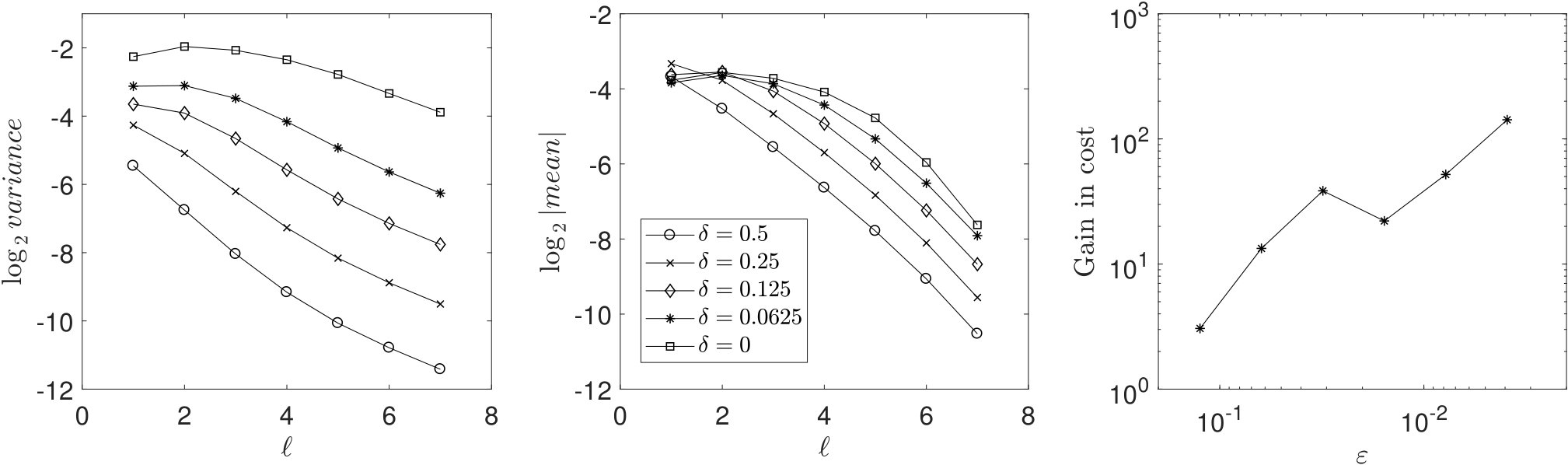 Figure 1
 Figure 2
 Figure 3
| Param. | Interpretation | Value |
|---|---|---|
| set-point | ||
| dead-band width | ||
| ambient temperature | ||
| power |
Peer Reviews
No public reviews on file for this paper yet. If you reviewed it on a platform where reviews are public (OpenReview, ICLR, NeurIPS, ICML), you can paste yours below so the community can read it here.
Videos
No videos yet. Explain this paper in a talk, walkthrough, or lecture? Add one.
Taxonomy
TopicsFormal Methods in Verification · Simulation Techniques and Applications · Advanced Control Systems Optimization
11institutetext: Max Planck Institute for Software Systems, Kaiserslautern, Germany
11email: {Sadegh,Rupak}@mpi-sws.org 22institutetext: Department of Statistics, University of Oxford, United Kingdom
22email: [email protected]
Authors’ Instructions
Multilevel Monte Carlo Method for Statistical
Model Checking of Hybrid Systems
Sadegh Esmaeil Zadeh Soudjani 11
Rupak Majumdar 11
Tigran Nagapetyan 22
Abstract
We study statistical model checking of continuous-time stochastic hybrid systems. The challenge in applying statistical model checking to these systems is that one cannot simulate such systems exactly. We employ the multilevel Monte Carlo method (MLMC) and work on a sequence of discrete-time stochastic processes whose executions approximate and converge weakly to that of the original continuous-time stochastic hybrid system with respect to satisfaction of the property of interest. With focus on bounded-horizon reachability, we recast the model checking problem as the computation of the distribution of the exit time, which is in turn formulated as the expectation of an indicator function. This latter computation involves estimating discontinuous functionals, which reduces the bound on the convergence rate of the Monte Carlo algorithm. We propose a smoothing step with tunable precision and formally quantify the error of the MLMC approach in the mean-square sense, which is composed of smoothing error, bias, and variance. We formulate a general adaptive algorithm which balances these error terms. Finally, we describe an application of our technique to verify a model of thermostatically controlled loads.
Keywords:
statistical model checking, formal verification, hybrid systems, continuous-time stochastic processes, multilevel Monte Carlo, reachability analysis
1 Introduction
Continuous-time stochastic hybrid systems (ct-SHS) are a natural model for cyber-physical systems operating under uncertainty [6, 8]. A ct-SHS has a hybrid state space consisting of discrete modes and, for each mode, a set of continuous states (called the invariant). In each mode, the continuous state evolves according to a stochastic differential equation (SDE) in continuous time. Transition from one discrete mode to another may be activated in two ways. The continuous state may hit the boundary of the invariant and make a forced transition according to a discrete stochastic transition kernel. Alternatively, the process may spontaneously change its discrete mode according to a continuous-time Markov chain whose rates depend on the hybrid state.
We consider quantitative analysis of temporal properties of ct-SHS [4, 3]. The fundamental analysis problem, called probabilistic reachability, consists in computing the probability that the state of a ct-SHS exits a given safe set within a given bounded time horizon. Since analytic solutions are not available, there are two common approaches. The first approach is numerical model checking that relies on the exact or approximate computation of the measure of the executions satisfying the temporal property. The second approach, called statistical model checking, relies on finitely many sample executions of the system, and employs hypothesis testing to provide confidence intervals for the estimate of the probability.
Statistical model checking has proven to be computationally more efficient than numerical model checking as it only requires the system to be executable. Thus, it can be applied to larger classes of systems and of specifications [25]. The main underlying assumption in all statistical model checking techniques is the ability to sample from the space of executions of the system. Unfortunately, we cannot compute exact simulations for the general class of ct-SHS due to the process evolution being continuous in both time and space. In this paper, we describe a statistical model checking approach to ct-SHS using the multilevel Monte Carlo (MLMC) method [18, 21], which does not require exact executions of the system.
Our procedure works as follows. First, we formulate the quantitative analysis problem as computing the distribution of the first exit time of the system from the given safe set. Then, we build a sequence of approximate models whose executions converge weakly (or in expectation) to the execution of the concrete system. Although these approximate models can be used separately in the classical setting of statistical model checking in order to compute estimates of the exit time, the MLMC method can take advantage of coupling between approximate executions with different time resolutions to provide better convergence rates.
An important challenge in applying the MLMC technique to the quantitative analysis of ct-SHS is that a discontinuous function is applied to the first exit time. While MLMC can be applied to discontinuous functions, the convergence rates we can guarantee are poor. We propose a smoothing step that replaces the discontinuous function with a continuous approximation and show that the replacement decreases the overall computation cost. Finally, we analyze the asymptotic computational cost of the MLMC approach for a given error bound. We propose an adaptive algorithm which balances errors due to bias, variance, and smoothing, and which tunes the hyperparameters of the algorithm on the fly.
We illustrate our technique on an example model of thermostatically controlled loads.
Related work. Formal definitions of various classes of continuous-time probabilistic hybrid models are presented in [28], together with a comparison. Over such models, [5] has formalized the notion of probabilistic reachability, [29] has proposed a computational technique based on convex optimization, [14] has provided discretization techniques with formal error bounds, and [15] has developed an approach based on satisfiability modulo theory. An alternative approach towards formal, finite approximations of continuous-time stochastic models is discussed in [35] and extended in [34] to switching diffusions. These approaches generally suffer from curse of dimensionality and are not applicable to large dimensional models.
For discrete-time stochastic hybrid models probabilistic reachability (and safety) has been fully characterized in [2] and computed via software tools [12, 11] that use finite abstractions. The methods can be extended to more general probabilistic temporal logics [30]. These techniques assume discrete-time dynamics and cannot be extended to ct-SHS.
An overview of statistical model checking techniques can be found in [25, 24, 23]. The paper [10] employs statistical model checking for verifying unbounded temporal properties. The paper [9] has discussed the use of importance sampling to address the issue of rare events in statistical verification of cyber-physical systems. A distributed implementation of statistical model checking is proposed in [7] and a set-oriented method for statistical verification of dynamical systems is presented in [31].
Employing multigrid ideas to reduce the computational complexity (in terms of expected number of arithmetic operations) of estimating an expected value using Monte Carlo path simulations is initially proposed in [18] in the context of stochastic differential equations. MLMC has a better asymptotic complexity and by its nature allows to build consecutive approximations, which can balance the bias and variance. The general paradigm with adequate modifications has shown significant gains in modeling jump-diffusion SDEs [33] and in fault tolerance applications [27]. A more detailed overview of applications of MLMC can be found in [19]. The MLMC for estimating distribution functions is described in the recent paper [17], which is adapted to our setting.
The article is structured as follows. In Section 2, we define the ct-SHS model and the probabilistic reachability problem. In Sections 3 and 4, we discuss the standard Monte Carlo technique and the MLMC method, respectively, and compare their convergence rates. We then discuss two technical modifications: applying a smoothing operator to the discontinuous function of exit time (Section 5) and an adaptive MLMC algorithm for estimating the hyperparameters (Section 6). In Section 7, we provide simulation results for an example.
2 Model Definition
We study statistical model checking for the rich class of continuous-time stochastic hybrid systems (ct-SHS).
2.1 Continuous-Time Stochastic Hybrid Systems
Definition 1
A continuous-time stochastic hybrid system is a tuple where the components are defined as follows.
States
is a countable set of discrete states (modes) and maps each mode to an open set , called the invariant for the mode . A state with and is called a hybrid state. The hybrid state space is defined as
[TABLE]
We write for the boundary of a set and define .
Evolution
is a vector field and is a matrix-valued function, with , where is the hybrid space defined in (1). For each , define the following SDE:
[TABLE]
where is an -dimensional standard Wiener process in a complete probability space. We assume functions and are bounded and Lipschitz continuous for all . The assumption ensures the existence and uniqueness of the solution of the SDEs in (2).
Initial State
is the initial state of the system;
Transition Kernel
is a discrete stochastic kernel which governs the switching between the SDEs defined in (2). That is, for all , we assume is measurable and, for all , the function is a discrete probability measure.
Intuitively, an execution of a ct-SHS starts in the initial state , and evolves according to the solution of the diffusion process (2) for the current mode until it hits the boundary of the invariant of the current mode for the first time. At this point, a new mode is chosen according to the transition kernel and the execution proceeds according to the solution of the diffusion process for , and so on.
We need the following definitions. Let be the solution of diffusion process (2) starting from . Define as the first exit time of from the set ,
[TABLE]
A stochastic hybrid process, describing the evolution of a ct-SHS, is obtained by the concatenation of diffusion processes together with a jumping mechanism given by a family of first exit times ; we make this formal in Definition 2.
Definition 2
A stochastic process is called an execution of ct-SHS if there exists a sequence of stopping times such that for all :
- •
is the initial state of ;
- •
for , is constant and is the solution of SDE
[TABLE]
where is the -dimensional standard Wiener process;
- •
where is the first exit time from the mode as defined in (3);
- •
The probability distribution of is governed by the discrete kernel and , where .
Remark 1
For simplicity of exposition, we have put the following restrictions on the ct-SHS model in Definition 1. First, the model includes only forced jumps activated by reaching the boundaries of the invariant sets and does not capture spontaneous jumps activated by Poisson processes. Second, the continuous state remains continuous at the switching times as declared in Definition 2. The approach of this paper is still applicable for ct-SHS models without these restrictions by modifying the time discretization scheme presented in Section 3.
2.2 Example: Thermostatically Controlled Loads
Household appliances such as water boilers/heaters, air conditioners, and electric heaters –-all referred to as thermostatically controlled loads (TCLs)-– can store energy due to their thermal mass. TCLs have been extensively studied [13, 22, 26] for their role in energy management systems. TCLs generally operate within a dead-band around a temperature set-point and are naturally modeled using ct-SHS. The temperature evolution in a cooling TCL can be characterized by the following SDE:
[TABLE]
where is the ambient temperature, is the energy transfer rate of the TCL, and and are the thermal resistance and capacitance, respectively. The noise term in (4) is a standard Wiener process. The model of the TCL has two discrete modes. When , we say the TCL is in the OFF mode at time , and when , we say it is in the ON mode.
The temperature of the cooling TCL is regulated by a control signal based on discrete switching as
[TABLE]
where denotes a temperature set-point and a dead-band. Together, and characterize an operating temperature range. The model can be described by the ct-SHS , where
- •
with the invariants and
- •
state space of the model
- •
for all
- •
for all
- •
is the Kronecker delta with .
2.3 Problem Definition
For a given random variable defined on the executions of a ct-SHS, we study the problem of estimating its distribution function.
Problem 1
Let be a real-valued random variable defined on the executions of ct-SHS . Estimate , the distribution of for a given .
Consider a ct-SHS with state space , a safe set , assumed to be measurable, and a time interval . The safety problem asks to compute the probability that the executions of will stay in during time interval . The safety problem is dual to the reachability problem and has a fundamental role in model checking for ct-SHS. By taking in Problem 1 to be the first exit time of the system from , we reduce the safety problem to Problem 1.
Problem 2 (Probabilistic Safety)
Compute the probability that an execution of the ct-SHS , with initial condition , remains within a measurable set during the bounded time horizon :
[TABLE]
where and .
Remark 2
The random variable defined in Problem 2 is in fact the first exit time of the system from the safe set and its distribution can be represented as the expectation of an indicator functional:
[TABLE]
Problem 3 (Specification of interest for TCL)
Although the switching mechanism (5) is designed to keep the temperature inside the interval , there is still a chance that the temperature goes out of this interval due to the Wiener process . Define a random variable . We aim to estimate the probability .
Analytic solution of Problems 1-3 is infeasible for the class of ct-SHS. Numerical computation of the solution has been investigated for restrictive subclasses of ct-SHS [32, 1]. In this work, we propose an approximate computation technique with a confidence bound. Our technique based on MLMC substantially improves the computational complexity of the standard Monte Carlo method. We first discuss standard Monte Carlo (SMC) method in Section 3 and then present the MLMC method in Section 4.
3 Standard Monte Carlo Method
In order to compute the quantities of interest in Problems 1-2 we need to estimate
[TABLE]
where is a function of the execution of ct-SHS , is the indicator function over the interval and is a one-dimensional random variable. The exact executions of and thus exact samples of are not available is general but it is possible to construct approximate executions and approximate samples that converge to the exact ones in a suitable sense.
Alg. 1 presents a state update routine based on the Euler-Maruyama method that can be used to construct approximate executions. Given the model and the current approximate state , this algorithm computes the approximate state for the next time step of size . Equation (8) in step 1 of the algorithm is the Euler-Maruyama approximation of the SDE (2). If is still inside the invariant of the current mode , then the mode remains unchanged and will be the next state (steps 2-3). Otherwise, in steps 5-6 is projected onto the boundary of the invariant and the mode is updated according to the discrete kernel .
Alg. 2 generates approximate executions of and approximate samples of using Alg. 1. The algorithm requires the model , the definition of as a function of the execution of of , and the time interval . The output of the algorithm is an approximate sample of random variable . In steps 1-2 the number of time steps is selected and the discretization time step is computed. In order to highlight the dependency of the algorithm to the parameter , we have opted to use in the representation as the superscript of the variables. We call the level of approximation which is nicely connected to the MLMC terminology discussed in Section 4.
Alg. 2 initializes the approximate execution in step 3 as according to the initial state of . Then the algorithm iteratively computes the next approximate state by sampling from the -dimensional standard normal distribution in step 5 and applying Alg. 1 to in step 6. Finally, step 9 constructs the continuous-time approximate execution as the piecewise constant version of the discrete execution , which enables the computation of by applying the definition of to (step 10).
Alg. 2 is parameterized by . Due to the nature of the Euler-Maruyama method in (8), we expect that the approximate samples converge to as in a suitable way. In fact, it is an unbiased estimator in the limit: The idea behind standard Monte Carlo (SMC) method is to use the empirical mean of as an approximation of . The SMC estimator has the form
[TABLE]
which is based on replications of . The replications can be generated by running Alg. 2 (with a fixed ) times, or running any other algorithm that generates such samples (cf. Alg. 4 in Section 4). The SMC method is summarized in Alg. 3, which approximates based on a general sampling algorithm . Note that Alg. 3 can be used for estimating not only with being the indicator function but also any other functional that can be deterministically evaluated using the executions over the time interval .
Owing to the randomized nature of algorithm embedded in Alg. 3, we quantify the quality of its outcome using mean squared error:111 We slightly abuse the notation and indicate by the mean square error of Alg. 3 with the embedded sampling algorithm .
[TABLE]
The mean square error is decomposed into two parts: Monte Carlo variance and squared bias error. The latter is a systematic error arising from the fact that we might not sample our random variable exactly, but rather use a suitable approximation, while the former error comes from the randomized nature of the Monte Carlo algorithm. The Monte Carlo variance (first term in (10)) is proportional to as
[TABLE]
The cost of Alg. 3 is typically taken to be the expected runtime in order to achieve a prescribed accuracy . A more convenient approach for theoretical comparison between different methods is to consider the cost associated to sampling algorithm ,
[TABLE]
which facilitates the definition of convergence rate of the algorithm.
Definition 3
We say that Alg. 3 based on sampling algorithm converges with rate if and if there exist constants such that
[TABLE]
Remark 3
The definition of convergence rate in (11) indicates that for a desired accuracy smaller convergence rate implies lower computational cost .
The following theorem presents the convergence rate of the SMC method presented in Alg. 3.
Theorem 3.1
Let denote the numerical approximation of the random variable according to an algorithm . Assume there exist positive constants such that for all
[TABLE]
Then the standard Monte Carlo method of Alg. 3 based on sampling algorithm converges with rate .
Remark 4
Recall the role of in step 2 of Alg. 2. Increasing results in an exponential increase in the number of time steps thus also in the number of samples. Therefore we have assumed in (12) an exponential bound on the increased cost and an exponential bound in the decreased bias as a function of .
Application to the TCL Case Study. We construct the approximate discrete-time executions as
[TABLE]
where is the sample from the standard normal distribution, , , and the discrete mode at any level is defined as with defined in (5). This discrete-time updating is slightly different from the Update function of Alg. 1, which can be interpreted as follows. Instead of continuous updating of mode, the control signal acts as a digital controller and updates the mode only at the discrete time steps. It is clear, that the cost of simulating one execution of (13) is proportional to the number of the discretization steps, thus setting the parameter in Theorem 3.1.
The values of constants in Theorem 3.1 depend on the regularity of the functional , sampling algorithm and other parameters. In the next section we propose to use MLMC method that improves the convergence rate and substantially reduces the computational complexity of the estimation. We discuss a smoothing in Section 5 that replaces the indicator function with a smoothed function and discuss its effect on the algorithm’s error.
4 Multilevel Monte Carlo Method
The multilevel Monte Carlo method (MLMC) relies on the simple observation of telescoping sum for expectation:
[TABLE]
where and correspond respectively to the coarsest and finest levels of numerical approximation. While any of the approximations can be used individually in Alg. 3 to approximate , instead, the MLMC method independently estimates each of the expectations on the right-hand side of (14) such that the overall variance is minimized for a given computational cost. The estimator of can be seen as a sum of independent estimators
[TABLE]
where is an estimator for based on samples, and are estimates for based on samples. As we saw in the MSC method of Section 3, the simplest forms for and are the empirical means over all samples:
[TABLE]
Using the assumption of having independent estimators and employing the telescoping sum (14) we can compute respectively the variance of and bias as
[TABLE]
The computation of in (16) requires the samples to be generated from a common probability space. We utilize the fact that sum of normal random variables is still normally distributed. Alg. 4 presents generation of approximate coupled samples for the random variable defined on the execution of a ct-SHS . As can be seen in steps 6-7 and 11, the approximate execution for the finer level is constructed exactly the same way as in Alg. 2 with time steps. The construction of approximate execution for the coarser level with is also similar except that the noise term in step 8 is obtained by taking the weighted sum of noise terms from the finer level . This choice preserves the properties of each approximation level while coupling the executions of levels thus also coupling approximate samples .
Now we are ready to present the MLMC method in Alg. 5. The method is parameterized by the number of levels , number of samples for each level , (which are gathered in ), and the initial number of time steps . Steps 2-3 performs the SMC method of Alg. 3 with embedded sampling algorithm 2 in order to estimate with samples at the initial level . Then the algorithm iteratively estimate in steps 6-7 using Alg. 3 with number of samples and with the embedded coupled sampling algorithm 4. The sum estimated quantity is reported in step 10 as the estimation of .
The next theorem gives the convergence rate of MLMC method presented in Alg. 5.
Theorem 4.1
Let denote the level numerical approximation of the random variable . Assume the independent estimators used in Alg. 5 satisfy
[TABLE]
for positive constants with . Then the MLMC method in Alg. 5 converges with rate
Assumptions in (17) are exactly the same as the ones used in Theorem 3.1. Assumptions in (20) put restriction on the statistical properties of the estimators : they first enables us to use the telescoping property (14) and the second ensures the exponentially decaying variance as a function of level . In compare with the convergence rate of SMC method in Theorem 3.1, the improvement is due to the non-zero factor which is the decaying rate of the variance of estimators.
Application to the TCL Case Study. We construct the approximate discrete-time executions for the finer lever as
[TABLE]
where is the sample from the standard normal distribution, , , and with defined in (5). The coupling, which means that we get the dynamics for based on the increments for , is done in a following way:
[TABLE]
where with . The fact that we have used the same Brownian increments from the finer level (21) in the courser level (22) lays the foundation of having nonzero value of in Theorem 4.1. The cost of simulating one approximate execution in (21)-(22) is proportional to the number of discretization steps, thus setting the parameter in Theorems 3.1-4.1.
Now that we have set up the MLMC method and the coupling technique that improves the convergence rate of the estimation, we focus on the following important problems associated with the approach:
Discontinuity of functional , leads to smaller values of and in Theorem 4.1. This results in larger convergence rate thus larger computational cost for a given accuracy . 2. 2.
The optimal choice of parameters , and the unknown constants in Theorem 4.1.
The first issue, discussed in Section 5, is resolved through smoothing, which replaces the discontinuous function with a smoothed function with Lipschitz constant proportional to . The second issue, discussed in Section 6, is resolved through an adaptive algorithm. This adaptive algorithm follows [20], and combines the smoothing of discontinuous functionals and the MLMC method. Note that we require an updated set of assumptions and include the search for parameter into the adaptive algorithm.
5 MLMC with Smoothed Indicator Function
The smoothing is based on the function , which are the rescaled translates of a function of the form
[TABLE]
Since we add a smoothing step, we need to update the MLMC estimator (15), derive new a MSE decomposition (instead of (10)) which incorporates the error due to the smoothing, and update Assumptions (17)-(20) in Theorem 4.1.
Note that function (23) is not the only possible choice for a smoothing function (see [20]), but in our experience this is the easiest to implement and numerically stable, while still providing significant gains in computational cost.
Recall that the MLMC method is based on a sequence of random variables, defined on a common probability space together with . The new MLMC method that includes smoothing is defined by
[TABLE]
with an independent family of -valued random variables for and such that equality in distribution holds for and , where we used the notation for the initial level . Note that (24) is the same as the MLMC estimator (15) except using the smoothing function instead of the indicator function . The next theorem gives the mean square error decomposition for (24).
Theorem 5.1
For , the error of in (24) with smoothing function (23) can be decomposed as
[TABLE]
The error terms in (25) are related to smoothing, bias, and variance, respectively. Note that as goes to zero, the Lipschitz constant for goes to infinity, which has to be taken into account. Hence the assumptions in Theorem 4.1 have to be updated. The theoretical analysis and updated assumptions are presented in [20].
6 Adaptive MLMC Algorithm
In this section we present an adaptive algorithm to find the optimal parameters for the MLMC method. For a given we wish to select the parameters of the MLMC algorithm such that its error is at most and its cost is as small as possible. Our approach to the selection of the replication numbers and of the maximal level follows [19].
The adaptive algorithm assumes no prior knowledge on the smoothing parameter , along with bias and variance dependencies on it. The smoothing parameter is chosen from the discrete set of values where . With a slight abuse of notation we put In order to achieve we have to assign certain proportions of to the three sources of the error introduced in (25). Specifically we wish to choose the parameters of our algorithm such that
[TABLE]
The MLMC algorithm is parameterized by the value for smoothing , the values of the maximal level , and the replication numbers . We always select and for . By the latter, we ensure a reasonable accuracy in certain estimates to be introduced below. We use to denote actual samples of the random variable and to denote the actual samples of the random vector for as opposed to which were used previously for their respective random variables.
Assumptions. Theorem 4.1 relies on the assumption of exponential upper bounds in (17)-(20), which in general might be difficult to verify. Instead in this section we study asymptotic upper bounds. For this purpose we use the following notation. For sequences of real numbers and positive real numbers we write if and write if We also replace assumptions (17)-(20) with the requirement that for every there exists such that
[TABLE]
This yields the following asymptotic upper bound for the bias at level
[TABLE]
We put with , the degree of polynomial in (23), and suppose that there exists such that \bigl{|}\mathbb{E}(g^{m}(Y))-\mathbb{E}(g^{m-1}(Y))\bigr{|}\approx c\cdot\delta_{m}^{4}. This yields the asymptotic upper bound for the smoothing error with parameter ,
[TABLE]
Our adaptive MLMC algorithm is based on the intuition that the asymptotic bounds (28) and (29) can be replaced by their corresponding inequalities ( instead of ), and estimators for means and variances can be assumed to be nearly exact.
Variance Estimation and Selection of the Replication Numbers. To estimate the expectations and variances we employ the empirical mean and variance
[TABLE]
We get that serves as an empirical upper bound for the variance of the MLMC algorithm with any choice of replication numbers . If, for the present choice of replication numbers, this bound is too large compared to the upper bound for in (26), i.e., if the variance constraint
[TABLE]
is violated, we determine new values of by minimizing subject to the constraint , which leads to
[TABLE]
and extra samples of and have to be generated accordingly.
Bias Estimation and Selection of the Maximal Level. For estimating we can use the values of already available from (30) for the levels . We estimate and in (27) by a least-squares fit, i.e., we take and to minimize
[TABLE]
While the value of is irrelevant, an upper bound for is given by , or, more generally, by with . This geometric upper bound can be used to set the stopping criterion of increasing the maximal level. Let us define
[TABLE]
The present value of is accepted as the maximal level, if the bias constraint
[TABLE]
is satisfied. Otherwise, is increased by one, and new samples will be generated.
Selection of the Smoothing Parameter. We wish to determine the smallest value of , i.e., the largest value of , such that
[TABLE]
is satisfied, which corresponds to the upper bound for in (26) together with (29). Initially we try . Actually, is approximated by , so the present value is accepted if
[TABLE]
The Adaptive Algorithm. We combine the above results and sum them up in Alg. 6, where the desired accuracy is the input.
7 Simulation Results
Recall Problem 3 where the goal is to estimate the probability . The random variable is defined as . We set the parameters of the TCL model (4)-(5) according to Table 1 and select the time horizon hour. We implement the MLMC Alg. 6 for target accuracies , where We set the parameters , in (26). With this choice we put less pressure on the smoothing error because the influence of the smoothing parameter on the variance and thus on the overal cost is severe. Due to the smoothing step we have to sample executions for the time duration of at least in order to evaluate the functional . With the selected values of and , sampling executions for hours is sufficient.
The result of the experiments is presented in Figure 1. The left and center plots show the impact of the smoothing coefficient on the variance and mean decays respectively based on runs of the algorithm. The data points of the plots with and with the indicator function are related to the SMC method. These plots indicate that the adaptive MLMC method is beneficial over SMC method due to the strong variance and mean decay with respect to level as well as the use of smoothing function instead of the indicator function.
The computational gain of the MLMC over SMC is presented on the right plot based on runs. The plot compares the expected cost of the SMC method with the estimated cost of the adaptive MLMC method. The cost of SMC method is given by (see Theorem 3.1), which bounds the cost of generating executions and evaluating functionals. We estimate the parameter through the precalculation and do not take into account the cost of estimating . In this way we assume the parameter is known in advance and make the comparison more in favor of the SMC method. The plot indicates larger computational gains for higher target accuracies (smaller ). Note that the curve in the right plot is not monotone because there is an additional cost of updating the smoothing coefficient, hence re-evaluating the functionals with the new value of . This additional cost has not been compensated by the MLMC gains as much in compare with the neighboring accuracies.
8 Conclusions
In this paper we studied the problem of statistical model checking of continuous-time hybrid systems that do not admit exact simulations. We employed multilevel Monte Carlo method and presented a smoothing step with tunable precision that replaces the desired discontinuous functional with a continuous approximation thus decreasing the overall computational effort of the approach. An adaptive algorithm was designed which balances the errors due to the bias, variance, and smoothing. The approach was demonstrated on the model of thermostatically controlled loads.
The reference list from the paper itself. Each links out to its DOI / PubMed record.
- 1[1] A. Abate, L. Bortolussi, M. Kwiatkowska, L. Cardelli, M. Ceska, and L. Laurenti. Reachability computation for switching diffusions: finite abstractions with certifiable and tuneable precision. In Hybrid Systems: Computation and Control , HSCC ’17, New York, NY, USA, 2017. ACM.
- 2[2] A. Abate, M. Prandini, J. Lygeros, and S. Sastry. Probabilistic reachability and safety for controlled discrete time stochastic hybrid systems. Automatica , 44(11):2724–2734, Nov 2008.
- 3[3] C. Baier, B. Haverkort, H. Hermanns, and J.-P. Katoen. Model-checking algorithms for continuous-time Markov chains. Trans. on Software Engineering , 29(6):524–541, June 2003.
- 4[4] C. Baier and J.-P. Katoen. Principles of Model Checking . MIT Press, 2008.
- 5[5] M.L. Bujorianu and J. Lygeros. Reachability questions in piecewise deterministic Markov processes. In O. Maler and A. Pnueli, editors, Hybrid Systems: Computation and Control , volume 2623 of Lecture Notes in Computer Science , pages 126–140. Springer Verlag, 2003.
- 6[6] M.L. Bujorianu and J. Lygeros. General stochastic hybrid systems: Modelling and optimal control. In in Proc. 43rd IEEE Conf. Decision Control , pages 1872–1877, 2004.
- 7[7] P. Bulychev, A. David, K.G. Larsen, A. Legay, M. Mikučionis, and D.B. Poulsen. Checking and Distributing Statistical Model Checking , pages 449–463. Springer, Berlin, Heidelberg, 2012.
- 8[8] C.G. Cassandras and J. Lygeros (Eds.). Stochastic Hybrid Systems . Number 24 in Control Engineering. CRC Press, Boca Raton, 2006.