Improving the Benjamini-Hochberg Procedure for Discrete Tests
Sebastian D\"ohler, Guillermo Durand (1), Etienne Roquain (1)((1), LPMA)

TL;DR
This paper introduces new modifications to the Benjamini-Hochberg procedure that account for data discreteness and signal strength, providing theoretical FDR control guarantees and demonstrating improved power in genomic data analysis.
Contribution
It develops theoretically guaranteed, discrete-aware FDR procedures that adapt to signal proportion, filling a gap in existing methods.
Findings
New FDR procedures control the false discovery rate under independence.
The methods show increased power in simulations and real genomic datasets.
The approach combines discreteness and signal proportion adaptively.
Abstract
To find interesting items in genome-wide association studies or next generation sequencing data, a crucial point is to design powerful false discovery rate (FDR) controlling procedures that suitably combine discrete tests (typically binomial or Fisher tests). In particular, recent research has been striving for appropriate modifications of the classical Benjamini-Hochberg (BH) step-up procedure that accommodate discreteness. However, despite an important number of attempts, these procedures did not come with theoretical guarantees. The present paper contributes to fill the gap: it presents new modifications of the BH procedure that incorporate the discrete structure of the data and provably control the FDR for any fixed number of null hypotheses (under independence). Markedly, our FDR controlling methodology allows to incorporate simultaneously the discreteness and the quantity of…
Click any figure to enlarge with its caption.
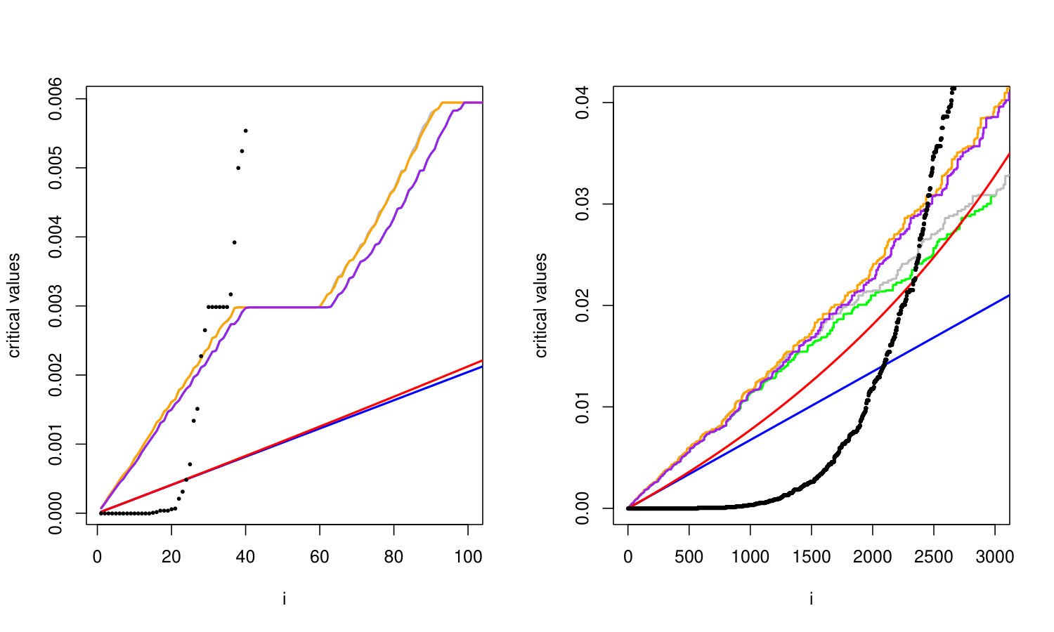 Figure 1
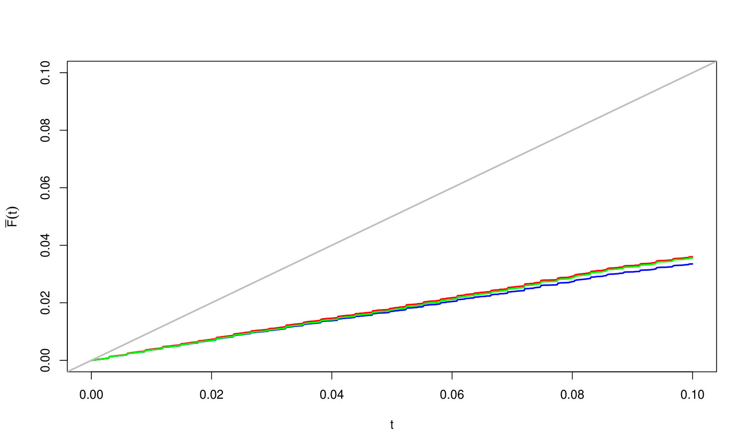 Figure 2
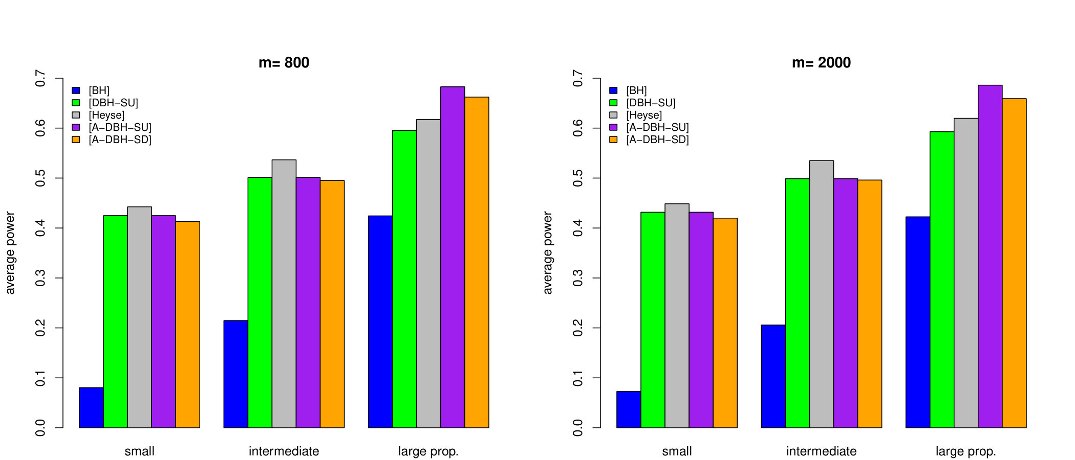 Figure 3
| Data set | [BH] | [DBH-SU] | [Heyse] | [A-DBH-SU] | [A-DBH-SD] |
|---|---|---|---|---|---|
| Pharmacovigilance | 24 | 27 | 27 | 27 | 27 |
| Arabidopsis methylation | 2097 | 2358 | 2379 | 2446 | 2453 |
| [BH] | [Heyse] | [DBH-SU] | [A-DBH-SU] | [A-DBH-SD] | ||||
|---|---|---|---|---|---|---|---|---|
| 800 | 80 | 144 | 0.15 | 0.0000 | 0.0004 | 0.0003 | 0.0003 | 0.0004 |
| 144 | 0.25 | 0.0004 | 0.0197 | 0.0177 | 0.0177 | 0.0135 | ||
| 144 | 0.4 | 0.0803 | 0.4425 | 0.4247 | 0.4247 | 0.4130 | ||
| 360 | 0.15 | 0.0000 | 0.0007 | 0.0006 | 0.0006 | 0.0007 | ||
| 360 | 0.25 | 0.0004 | 0.0244 | 0.0209 | 0.0209 | 0.0153 | ||
| 360 | 0.4 | 0.0803 | 0.4529 | 0.4509 | 0.4509 | 0.4487 | ||
| 576 | 0.15 | 0.0000 | 0.0009 | 0.0007 | 0.0007 | 0.0008 | ||
| 576 | 0.25 | 0.0004 | 0.0343 | 0.0259 | 0.0259 | 0.0231 | ||
| 576 | 0.4 | 0.0803 | 0.5367 | 0.4741 | 0.4741 | 0.4999 | ||
| 240 | 112 | 0.15 | 0.0000 | 0.0003 | 0.0003 | 0.0003 | 0.0002 | |
| 112 | 0.25 | 0.0005 | 0.0276 | 0.0249 | 0.0249 | 0.0157 | ||
| 112 | 0.4 | 0.2148 | 0.5365 | 0.5012 | 0.5012 | 0.4951 | ||
| 280 | 0.15 | 0.0000 | 0.0003 | 0.0003 | 0.0003 | 0.0002 | ||
| 280 | 0.25 | 0.0005 | 0.0315 | 0.0272 | 0.0272 | 0.0175 | ||
| 280 | 0.4 | 0.2147 | 0.5758 | 0.5536 | 0.5536 | 0.5495 | ||
| 448 | 0.15 | 0.0000 | 0.0005 | 0.0003 | 0.0003 | 0.0004 | ||
| 448 | 0.25 | 0.0005 | 0.0372 | 0.0308 | 0.0308 | 0.0207 | ||
| 448 | 0.4 | 0.2145 | 0.5920 | 0.5741 | 0.5741 | 0.5775 | ||
| 640 | 32 | 0.15 | 0.0000 | 0.0002 | 0.0002 | 0.0002 | 0.0002 | |
| 32 | 0.25 | 0.0010 | 0.0378 | 0.0341 | 0.0341 | 0.0174 | ||
| 32 | 0.4 | 0.4243 | 0.6174 | 0.5955 | 0.6828 | 0.6621 | ||
| 80 | 0.15 | 0.0000 | 0.0002 | 0.0002 | 0.0002 | 0.0002 | ||
| 80 | 0.25 | 0.0010 | 0.0388 | 0.0347 | 0.0347 | 0.0179 | ||
| 80 | 0.4 | 0.4242 | 0.6282 | 0.6128 | 0.6841 | 0.6638 | ||
| 128 | 0.15 | 0.0000 | 0.0002 | 0.0002 | 0.0002 | 0.0002 | ||
| 128 | 0.25 | 0.0010 | 0.0400 | 0.0354 | 0.0354 | 0.0183 | ||
| 128 | 0.4 | 0.4240 | 0.6353 | 0.6265 | 0.6854 | 0.6656 | ||
| 2000 | 200 | 360 | 0.15 | 0.0000 | 0.0002 | 0.0002 | 0.0002 | 0.0002 |
| 360 | 0.25 | 0.0001 | 0.0156 | 0.0142 | 0.0142 | 0.0100 | ||
| 360 | 0.4 | 0.0730 | 0.4486 | 0.4317 | 0.4317 | 0.4197 | ||
| 900 | 0.15 | 0.0000 | 0.0002 | 0.0002 | 0.0002 | 0.0002 | ||
| 900 | 0.25 | 0.0001 | 0.0192 | 0.0166 | 0.0166 | 0.0125 | ||
| 900 | 0.4 | 0.0730 | 0.4517 | 0.4511 | 0.4511 | 0.4509 | ||
| 1440 | 0.15 | 0.0000 | 0.0003 | 0.0002 | 0.0002 | 0.0002 | ||
| 1440 | 0.25 | 0.0001 | 0.0286 | 0.0211 | 0.0211 | 0.0165 | ||
| 1440 | 0.4 | 0.0730 | 0.5402 | 0.4684 | 0.4684 | 0.4984 | ||
| 600 | 280 | 0.15 | 0.0000 | 0.0002 | 0.0002 | 0.0002 | 0.0002 | |
| 280 | 0.25 | 0.0001 | 0.0239 | 0.0213 | 0.0213 | 0.0115 | ||
| 280 | 0.4 | 0.2058 | 0.5350 | 0.4988 | 0.4988 | 0.4960 | ||
| 700 | 0.15 | 0.0000 | 0.0002 | 0.0002 | 0.0002 | 0.0002 | ||
| 700 | 0.25 | 0.0001 | 0.0290 | 0.0239 | 0.0239 | 0.0132 | ||
| 700 | 0.4 | 0.2058 | 0.5750 | 0.5590 | 0.5590 | 0.5516 | ||
| 1120 | 0.15 | 0.0000 | 0.0002 | 0.0002 | 0.0002 | 0.0002 | ||
| 1120 | 0.25 | 0.0001 | 0.0350 | 0.0283 | 0.0283 | 0.0157 | ||
| 1120 | 0.4 | 0.2057 | 0.5908 | 0.5739 | 0.5739 | 0.5761 | ||
| 1600 | 80 | 0.15 | 0.0000 | 0.0001 | 0.0001 | 0.0001 | 0.0000 | |
| 80 | 0.25 | 0.0003 | 0.0379 | 0.0342 | 0.0342 | 0.0126 | ||
| 80 | 0.4 | 0.4223 | 0.6196 | 0.5928 | 0.6860 | 0.6591 | ||
| 200 | 0.15 | 0.0000 | 0.0001 | 0.0001 | 0.0001 | 0.0000 | ||
| 200 | 0.25 | 0.0003 | 0.0387 | 0.0351 | 0.0351 | 0.0131 | ||
| 200 | 0.4 | 0.4222 | 0.6281 | 0.6152 | 0.6869 | 0.6602 | ||
| 320 | 0.15 | 0.0000 | 0.0001 | 0.0001 | 0.0001 | 0.0000 | ||
| 320 | 0.25 | 0.0003 | 0.0396 | 0.0360 | 0.0360 | 0.0137 | ||
| 320 | 0.4 | 0.4220 | 0.6327 | 0.6278 | 0.6877 | 0.6617 |
Peer Reviews
No public reviews on file for this paper yet. If you reviewed it on a platform where reviews are public (OpenReview, ICLR, NeurIPS, ICML), you can paste yours below so the community can read it here.
Videos
No videos yet. Explain this paper in a talk, walkthrough, or lecture? Add one.
Taxonomy
TopicsGenetic Associations and Epidemiology · Statistical Methods in Clinical Trials · Statistical Methods and Inference
Improving the Benjamini-Hochberg Procedure for Discrete Tests
Sebastian Döhlerlabel=e1][email protected] [ Darmstadt University of Applied Sciences
D-64295 Darmstadt, Germany
E-mail: [email protected]
Guillermo Durandlabel=e2][email protected] [
Sorbonne Universités, UPMC
4, Place Jussieu, 75252 Paris cedex 05, France
Email: [email protected]
Etienne Roquainlabel=e3][email protected] [ Sorbonne Universités, UPMC
4, Place Jussieu, 75252 Paris cedex 05, France
E-mail: [email protected]
Abstract
To find interesting items in genome-wide association studies or next generation sequencing data, a crucial point is to design powerful false discovery rate (FDR) controlling procedures that suitably combine discrete tests (typically binomial or Fisher tests). In particular, recent research has been striving for appropriate modifications of the classical Benjamini-Hochberg (BH) step-up procedure that accommodate discreteness. However, despite an important number of attempts, these procedures did not come with theoretical guarantees. The present paper contributes to fill the gap: it presents new modifications of the BH procedure that incorporate the discrete structure of the data and provably control the FDR for any fixed number of null hypotheses (under independence). Markedly, our FDR controlling methodology allows to incorporate simultaneously the discreteness and the quantity of signal of the data (corresponding therefore to a so-called -adaptive procedure). The power advantage of the new methods is demonstrated in a numerical experiment and for some appropriate real data sets.
false discovery rate,
discrete hypothesis testing,
type I error rate control,
adaptive procedure,
step-up algorithm,
step-down algorithm,
keywords:
\startlocaldefs\endlocaldefs
and
and
Multiple testing procedures are now routinely used to find significant items in massive and complex data. An important focus has been given to methods controlling the false discovery rate (FDR) because this scalable type I error rate “survives” to high dimension. Since the original procedure of Benjamini and Hochberg (1995), much effort has been undertaken to design FDR controlling procedures that adapt to various underlying structures of the data, such as the quantity of signal, the signal strength and the dependencies, among others.
In this work, we deal with adaptation to discrete data. This type of data arises in many relevant applications, in particular when data are represented by counts. Examples can be found in clinical studies (see e.g. Westfall and Wolfinger (1997)), genome-wide association studies (GWAS) (see e.g. Dickhaus et al. (2012)) and next generation sequencing data (NGS) (see e.g. Chen and Doerge (2015b)). It is well known (see e.g. Westfall and Wolfinger (1997)) that using discrete test statistics can generate a severe power loss, already at the stage of the single tests. A consequence is that using “blindly” the BH procedure with discrete -values will control the FDR in a too conservative manner. Therefore, more powerful procedures that avoid this conservatism are much sought after in applications, see for instance Karp et al. (2016), van den Broek et al. (2015) and Dickhaus et al. (2012).
In the literature, building multiple testing procedures that take into account the discreteness of the test statistics has a long history that can be traced back to Tukey and Mantel (1980). Some null hypotheses can be a priori excluded from the study because the corresponding tests are unable to produce sufficiently small -values. This results in a multiplicity reduction that should increase the power. While this idea has been exploited in Tarone (1990) and in a more general manner in Westfall and Wolfinger (1997) for family-wise error rate, an attempt has been made for FDR later in Gilbert (2005). More recently, Heyse (2011) has proposed a more powerful solution, relying on the following averaged cumulative distribution function (c.d.f.):
[TABLE]
where each corresponds to the c.d.f. of the -th test -value under the null hypothesis. To illustrate the potential benefit of using , Figure 1 displays this function for the pharmacovigilance data from Heller and Gur (2011) (see Section 4 for more details). The critical values of the Heyse procedure can be obtained by inverting at the values . Thus, the smaller the -values, the larger the critical values. Here, Heyse critical values improve the BH critical values roughly by a factor 3, thereby yielding a potentially strong rejection enhancement. Furthermore, since the functions ’s are known, so is . Hence, the user has a good prior idea of the improvements reachable by this discrete approach. Unfortunately, the Heyse procedure does not rigorously control the FDR in general; counter-examples are provided in Heller and Gur (2011) and Döhler (2016).
Meanwhile, different solutions have been explored by modifying directly the -values, either by randomization (see Habiger (2015) and references therein), or by shrinking them to build so-called midP-values (see Heller and Gur (2011) and references therein). Other approaches incorporate discreteness to obtain less conservative FDR estimates, see, e.g., Pounds and Cheng (2006), or by combining grouping and weighting approaches, see Chen and Doerge (2015b).
Overall, although many new procedures have been proposed in the literature, only few of them have been proved to achieve a rigorous FDR control under standard conditions, especially in the finite sample case. To the best of our knowledge, we can only refer to the discretised version of the procedure of Benjamini and Liu (1999) introduced by Heller and Gur (2011) and to the asymptotic work of Ferreira (2007). Chen and Doerge (2015b) sum up the status quo by noting that ’…how to derive better FDR procedures in the discrete paradigm remains an urgent but still unresolved problem.’ This paper offers a solution by presenting new procedures that achieve both theoretical validity and good practical performance.
The paper is organised as follows: after having precisely defined the setting in Section 1, we introduce in Section 2 new procedures relying on the following modifications of the function
[TABLE]
(with the convention ), where an appropriate choice of is made. To feel how light these modifications are, Figure 1 displays these functions and shows they are very close to the original for small values of . In addition, we also introduce more powerful “adaptive” versions, meaning that the derived critical values are designed in a way that “implicitly estimate” the overall proportion of true null hypotheses and thus may outperform the original Heyse procedure. Next, in Section 3, we establish rigorous FDR control of the corresponding non-adaptive and adaptive procedures under standard conditions. Our proofs rely on new bounds on FDR that generalise some prominent results of the multiple testing literature. These bounds are the main mathematical contributions of the paper and are interesting in their own right, beyond the discrete setting. Also, to explore in detail the improvement of our procedures, we analyse both real and simulated data in Sections 4 and 5. Finally, while the proofs are given in appendix (together with some additional procedures), complementary results are provided in Appendix C.
1 Preliminaries
1.1 General model
Let us observe a random variable , defined on a probabilistic space and valued in an observation space . We consider a set of possible distributions for the distribution of and we denote the true one by . We assume that null hypotheses , , are available for and we denote the corresponding set of true null hypotheses by \mathcal{H}_{0}(P)=\{1\leq i\leq m\>:\>\mbox{H_{0,i}P}\}. We also denote by the number of true nulls.
We assume that the user has at hand a set of -values to test each null, that is, a set of random variables , valued in . Throughout the paper, we also make the important (but classical) assumption that the -values , , are mutually independent.
Now, we denote , where for each , the function
[TABLE]
is assumed to be known. Note that we necessarily have non decreasing, , and we add the technical condition . Loosely, each corresponds to the cumulative distribution of under the null. Above, we have taken the supremum to cover the case where the null hypothesis is composite: in that situation, each is adjusted according to the least favorable configuration within the null .
Here are some conditions on that will be useful to compare some of the studied procedures (these conditions are not assumed in our results unless explicitly mentioned):
[TABLE]
Condition (2) ensures that the -values have marginals stochastically lower-bounded by a uniform variable under the null, called a super-uniform distribution in the sequel. This is the classical setting which is used in most of the work dealing with FDR controlling theory, see, e.g., Benjamini and Hochberg (1995). Condition (3) is more restrictive: if each null hypothesis is a singleton, it is equivalent to the -values having uniform marginals under the null.
1.2 Discrete and continuous modelling
In order to describe the overall support of -value distributions we assume one of the two following situations to be at hand throughout the paper (except in Section 3 which is written in a more general manner):
- •
Continuous case: for all , is continuous. In that case, we let , and is the overall -value support.
- •
Discrete case: each -value (both under the null and alternative) takes values in some finite set , where and is an increasing sequence (with , ). We denote the overall -value support.
The continuous setting is typically valid in situations where the -values are calibrated from test statistics having a continuous distribution under the null. In this situation, (3) is often satisfied. The discrete setting typically arises in situations where the -values are calibrated from test statistics having a finitely supported distribution under the null. In this situation, we generally have that (3) holds true only on the support of , that is,
[TABLE]
In the discrete framework, let us underline that while (4) will typically hold, the equality , will fail in general because contains points of for . Then defined by (1) will be smaller than in general (see Figure 1), which is exactly the property that we want to exploit in this paper.
To illustrate the above framework, we provide below two simple examples (for more advanced examples, see for instance Chen and Doerge (2015b)).
Example 1.1* (Gaussian testing).*
Observe with independent coordinates and marginals , where is the parameter of interest, . In that situation, a possible hypothesis testing problem is to consider the nulls “” against “”. Then , , is a family of -values satisfying (3) (where denotes the c.d.f. of a standard Gaussian variable).
Example 1.2* (Binomial testing).*
Observe with independent coordinates and marginals , where is known and is the parameter of interest, . In that situation, a possible hypothesis testing problem is to consider the nulls “” against “”. Then , , define a family of -values where is the upper-tail distribution function of a binomial distribution of parameters . The support of the -values under the null and alternative is covered by letting and , . We merely check in that case that (3) is violated while (2) and (4) hold.
1.3 Step-wise procedures
First define a critical value sequence as any nondecreasing sequence (with by convention).
The step-up procedure of critical value sequence , denoted by , rejects the -th hypothesis if , with where denote the ordered -values (with the convention ).
The step-down procedure of critical value sequence , denoted by , rejects the -th hypothesis if , with It is straightforward to check that, for the same set of critical values, the step-up version always rejects more hypotheses than the step-down version. More comments and illustrations on step-wise procedures can be found in Blanchard et al. (2014) and Dickhaus (2014), among others.
1.4 False discovery rate
We measure the quantity of false positives of a step-up (resp. step-down) procedure by using the false discovery rate (FDR), introduced and popularised by Benjamini and Hochberg (1995), which is defined as the averaged proportion of errors among the rejected hypotheses. More formally, for some procedure rejecting the -th hypothesis if (for some threshold ), we let
[TABLE]
The main contribution of this work is to propose procedures that control the FDR at a prescribed level and that incorporate the knowledge of the ’s in a way that increases the number of discoveries.
2 Procedures
In this section we briefly review some existing methods for FDR control and introduce our new procedures.
2.1 Existing methods
We use the following methods as starting points for constructing new procedures.
[BH]: the seminal procedure proposed in Benjamini and Hochberg (1995), corresponding to the step-up procedure , with critical values , ;
- -
[BR-]: an adaptive version of the BH procedure that was proposed in Blanchard and Roquain (2009), corresponding to the step-up procedure , with critical values
[TABLE]
- -
[GBS]: an adaptive version of the BH procedure that has been proposed in Gavrilov et al. (2009), corresponding to the step-down procedure , with critical values
[TABLE]
- -
[Heyse]: the step-up procedure using critical values given by
[TABLE]
where is defined by (1). This procedure was proposed in Heyse (2011).
The rationale behind the critical values of [BR-] and [GBS] is that they are intended to mimic the oracle critical values , , which are less conservative than those of [BH] when is not close to , see, e.g., Benjamini et al. (2006); Blanchard and Roquain (2009) for more details on adaptive procedures.
Let us now comment on [Heyse]. First, in the continuous setting where (2) holds, , , and thus the critical values given by (8) satisfy , , which means that [Heyse] rejects at least as many hypotheses as [BH]. When (3) additionally holds, we have , , and the two critical value sequences are the same. Second, in the discrete setting where (2) holds, is finite and is not necessarily greater than anymore. However, [Heyse] is also less conservative (or equal) than [BH] in the latter case, as stated in the following result (proved in Appendix C for completeness).
Lemma 2.1**.**
Consider the model of Section 1.1 assuming (2), both in the continuous and discrete setting described in Section 1.2. Then the set of nulls rejected by [Heyse] is larger than the one of [BH] (almost surely). Furthermore, under (4), these two rejection sets are equal (almost surely) if for all .
The equality case of Lemma 2.1 was provided in Proposition 2.3 of Heller and Gur (2011), who presented it as a limitation of Heyse procedure in the discrete case. However, we argue that the condition for all is a somehow extreme configuration which is rarely met in practice (in the discrete case). More typically, the ’s have an heterogeneous structure implying that is smaller than (see Figure 1). This entails that [Heyse] can substantially improve [BH] (see Figure 2).
While [Heyse] incorporates the knowledge of the ’s in a natural way (see also Remark 2.2 below), it is not correctly calibrated for a rigorous FDR control: as shown in Heller and Gur (2011); Döhler (2016), it fails to control the FDR in general. We propose suitable modifications of [Heyse] in the next sections.
Remark 2.2* (Empirical Bayes point of view on the Heyse procedure).*
We claim that [Heyse] corresponds to a suitable empirical Bayes procedure. To see this, consider the “binomial example” of Section 1.2, but assume now that the counts are observed from a sample i.i.d. of a priori distribution . Unconditionally, the -values , , are thus i.i.d. with c.d.f. where is the c.d.f. jumping at each with , . This suggests to normalise the -values as which leads to the step-up procedure with critical values . Following an empirical Bayes approach, the prior can be estimated by , which gives rise to the estimator of defined by which is equal to given by (1). Hence, the corresponding (empirical Bayes) step-up procedure reduces to [Heyse].
2.2 Two new methods
We now present two procedures that aim at correcting [Heyse] :
[DBH-SU]: the step-up procedure using the critical values defined in the following way:
[TABLE]
- -
[DBH-SD]: the step-down procedure using the critical values defined in the following way :
[TABLE]
[DBH-SU] can be seen as a correction of [Heyse]: the correction term in the critical values (10) lies in the additional denominator . A consequence is that [DBH-SU] can be more conservative than [BH]. However, the magnitude of this phenomenon is always small, as the next lemma shows (proved in Appendix C for completeness).
Lemma 2.3**.**
Under the conditions of Lemma 2.1, the set of nulls rejected by [DBH-SU] contains the one of [BH] taken at level (almost surely).
For [DBH-SD], the following result can be established.
Lemma 2.4**.**
Under the conditions of Lemma 2.1, the set of nulls rejected by [DBH-SD] contains the one of the step-down procedure with critical values , (almost surely).
From (10) and (11) it is clear that the critical values of [DBH-SD] are always at least as large as those for [DBH-SU]. However, since the step-up direction is more powerful than the step-down direction (see Section 1.3) neither of the two generally dominates the other one.
Remark 2.5*.*
We may ask whether we can construct a uniform improvement of [BH] that incorporate the ’s. There is indeed such a procedure (see procedure [RBH] in Appendix A.1 for more details). However, the improvement brought by the ’s information is less substantial than for [DBH-SU], so we have chosen to omit [RBH] from the main stream of the paper.
2.3 Adaptive versions
In this section, we define adaptive versions of [DBH-SU] and [DBH-SD] in the following way:
[A-DBH-SU]: the step-up procedure using the critical values defined in the following way: as in (9) and for ,
[TABLE]
where each denotes the -th largest elements of the set .
- -
[A-DBH-SD]: the step-down procedure using the critical values defined in the following way :
[TABLE]
where each denotes the -th largest elements of the set .
Note that the critical values of [A-DBH-SU] and [A-DBH-SD] are clearly larger than or equal to those of their non-adaptive counterparts [DBH-SU] and [DBH-SD], respectively. This means that the adaptive versions are always less conservative.
The following result establishes a connection of the adaptive procedures to the [BR-] and [GBS] procedures (proved in Appendix C for completeness).
Lemma 2.6**.**
Under the conditions of Lemma 2.1, the following holds:
- (i)
the set of nulls rejected by [A-DBH-SU] contains the one of [BR-] (almost surely), where is taken equal to (9);
- (ii)
the set of nulls rejected by [A-DBH-SD] contains the one of [GBS] (almost surely);
The above lemma ensures that the user can incorporate the knowledge of the ’s in adaptive procedures with a “no loss” guarantee with respect to [BR] and [GBS]. This is a somehow striking fact, coming loosely from a “fortunate marriage” between the proof technics of discreteness theory and adaptation theory.
Remark 2.7*.*
We may ask whether we can build a procedure that is a uniform improvement of [BR-], for any fixed value of . We propose a solution in Appendix A.2, called [DBR-]. It does not improve uniformly [DBH-SU], but is an interesting variant of [A-DBH-SU].
3 New FDR bounds
In this section, we present new FDR bounds which are the main mathematical contributions of this paper and that are of independent interest. They generalise some classical bounds from super-uniform null distributions to arbitrary heterogeneous (not necessarily discrete) null distributions, and immediately yield FDR control of our new procedures.
3.1 Results
First, remember that the model of Section 1.1 basically only assume independence between the -values (and not super-uniformity of the null distribution). The following result holds.
Theorem 3.1**.**
In the model of Section 1.1, for any critical values , and for all , we have
[TABLE]
The proof of Theorem 3.1 is deferred to Appendix B. It combines several techniques: the first tool is an expression of the FDR introduced by Ferreira (2007) (step-up case) and Roquain and Villers (2011) (step-down case). A second idea comes from the work Blanchard and Roquain (2009) (step-up case) and Gavrilov et al. (2009) (step-down case), which introduced a new term (here, the denominator ) to make the adaptive argument works fine. Finally, another inspiration is the study of Roquain and van de Wiel (2009) and Döhler (2016) that allowed to deal with heterogeneous FDR thresholding. Let us underline that the obtained proof is especially concise, which means that these different techniques fit together perfectly well, which is perhaps surprising at first glance, see Appendix B.3.
Next, let us note that taking the maximum over the subset in (14) and (15) allows us to adapt to the unknown number of true null hypotheses: loosely, if is the number of rejections, corresponds to the acceptation set (hence of cardinality ), which “estimates” and thus the sums in (14) and (15) are indexed by a set “close” to the unknown set . Taking the maximum then corresponds to account for the least favorable possible .
Finally, let us underline again that the above bounds do not use the super-uniformity of the ’s which makes them quite general and flexible tools. As a case in point, consider mid--values which were introduced by Lancaster (1961) and are sometimes used for analysing discrete data (see e.g. Karp et al. (2016)). These -values are no longer super-uniform under the null hypotheses, however our theorem can accomodate such distributions in a natural way to still yield valid FDR controlling procedures. In addition, note that our bounds can be useful outside the discrete setting, when the ’s are continuous but with flat parts, see the (toy) Example 3.3 below.
3.2 Rationale and relation to previous work
Let us now give some intuition behind these bounds by showing how it allows to cover previous work in the literature.
First, assuming the super-uniformity for all and , then these bounds entail
[TABLE]
which immediately recover the fact that [BH], [BR-] (with ) and [GBS] all control the FDR at level . To this respect, bounds (16), (17) and (18) encompass Theorem 3.1 of Benjamini and Hochberg (1995), Theorem 9 of Blanchard and Roquain (2009) and Theorem 1.1 of Gavrilov et al. (2009), respectively.
Second, by removing the adaptative part of the bounds, that is, by replacing by , we obtain the simpler but more conservative bounds
[TABLE]
where and are defined in the introduction, see also Figure 1. These variants illustrate perhaps more intuitively how the Heyse-type procedures take advantage of the heterogeneous structure: if some of the ’s are really small, they will not contribute much into (or ), offering some additional room for the other ’s.
Finally, these bounds immediately imply that our new procedures enjoy the desired FDR controlling property.
Corollary 3.2**.**
*In the model of Section 1.1, both in the continuous and discrete setting described in Section 1.2, the procedures [DBH-SU]; [DBH-SD]; [A-DBH-SU]; [A-DBH-SD] all control the FDR at level . *
Example 3.3*.*
Assume that the hypotheses are structured in non-overlapping groups , and , each of cardinality (assumed to be an integer). Assume that is equal to if , [math] if , and (); (); (), if . Then the bound (20) becomes (for ):
[TABLE]
which entails a new step-down FDR controlling procedure by taking such that the above expression is equal to . For small, we get which yields to a procedure close to a step-down version of [BH]. It thus controls the FDR even though the super-uniformity of the -values is violated. In particular, this illustrates that our methodology exceeds the scope of discrete tests.
4 Empirical data
To illustrate the performance of FDR-controlling procedures for discrete data, we analyse two benchmark data sets which have also been used in previous publications. In what follows, our main goal is to compare the performance of the new procedures [DBH-SU], [A-DBH-SU] and [A-DBH-SD] to the classical [BH] procedure. As a further benchmark we also include [Heyse] in the analysis. All analyses were performed using the R language for statistical computing (R Core Team, 2016).
4.1 Pharmacovigilance data
This data set is derived from a database for reporting, investigating and monitoring adverse drug reactions due to the Medicines and Healthcare products Regulatory Agency in the United Kingdom. It contains the number of reported cases of amnesia as well as the total number of adverse events reported for each of the drugs in the database. For more details we refer to Heller and Gur (2011) and to the accompanying R-package ’discreteMTP’ (Heller et al., 2012), which also contains the data. Heller and Gur (2011) investigate the association between reports of amnesia and suspected drugs by performing for each drug a Fisher’s exact test (one-sided) for testing association between the drug and amnesia while adjusting for multiplicity by using several (discrete) FDR procedures.
4.2 Next generation sequencing data
We also revisit the next generation sequencing (NGS) count data analysed by Chen and Doerge (2015b), to which we also refer for more details. More specifically, we reanalyse the methylation data set for cytosines of Arabidopsis in Lister et al. (2008) which is part of the R-package ’fdrDiscreteNull’ (Chen and Doerge, 2015a). This data set contains the counts for a biological entity under two different biological conditions or treatments. Following Chen and Doerge (2015b), genes whose treatment-wise total counts are positive but row-total counts are no greater than 100 are analysed using the exact binomial test, see Chen and Doerge (2015b).
4.3 Results
Table 1 summarises the number of discoveries for the pharmacovigilance and NGS data when using the respective FDR procedures at level .
Compared to the classical FDR controlling procedures, the new procedures are able to detect three additional candidates linking amnesia and drugs in the pharmacovigilance data. Note also that for this data, they reject the same number of hypotheses as [Heyse], even though [Heyse] is not correctly calibrated for FDR control. For the Arabidopsis data, the new procedures improve considerably on [BH]. Moreover, there is a clear separation between the adaptive and non-adaptive procedures.
Figure 2 illustrates graphically the data and the critical constants of the involved multiple testing procedures.
In particular, the benefit of taking discreteness into account becomes more apparent: for the pharmacovigilance data, the discrete critical values are considerably (by a factor of ) larger than their respective classical counterparts. This leads to more powerful procedures. For the NGS data, we can observe quite clearly that the [DBH-SU] critical constants are dominated by the [A-DBH-SU] constants, as explained in Section 2. This leads to roughly 100 additional rejections. Again, the discrete critical values are considerably larger than their respective classical counterparts. In 2.2 we mentioned that the correction factor , introduced for guaranteeing FDR control of [DBH-SU], may lead to a procedure which is more conservative than [BH]. However, Figure 2 shows that – at least for the data sets considered here – this risk is by far compensated by the benefit of taking discreteness adequately into account.
5 Simulation study
We now investigate the power of the procedures from the previous section in a simulation study similar to those described in Gilbert (2005), Heller and Gur (2011) and Döhler (2016). Again, we focus on comparing the performance of the new discrete procedures to [BH].
5.1 Simulated Scenarios
We simulate a two-sample problem in which a vector of independent binary responses (“adverse events”) is observed for each subject in two groups, where each group consists of subjects. Then, the goal is to simultaneously test the null hypotheses “”, , where and are the success probabilities for the th binary response in group 1 and 2, respectively. We take where and data are generated so that the response is at positions for both groups, at positions for both groups and at positions for group 1 and at positions for group 2 where represents weak, moderate and strong effects respectively. The null hypothesis is true for the and positions while the alternative hypothesis is true for the positions. We also take different configurations for the proportion of false null hypotheses, is set to be , and of the value of , which represents small, intermediate and large proportion of effects (the proportion of true nulls is , , , respectively). Then, is set to be , and of the number of true nulls (that is, ) and is taken accordingly as .
For each of the 54 possible parameter configurations specified by and , Monte Carlo trials are performed, that is, data sets are generated and for each data set, an unadjusted two-sided -value from Fisher’s exact test is computed for each of the positions, and the multiple testing procedures mentioned above are applied at level . The power of each procedure was estimated as the fraction of the false null hypotheses that were rejected, averaged over the simulations. For random number generation the R-function rbinom was used. The two-sided -values from Fisher’s exact test were computed using the R-function fisher.test.
5.2 Results
We have computed the (average) power of the five procedures under investigation in all the scenarios (see Table 1 in Appendix C for the full display). For weak and moderate effects, i.e. and , none of the procedure possesses relevant power. For strong effects, the results are summarised in Figure 3. (Since the power of the discrete procedures is slightly increasing in for fixed and , we present – in order to avoid over-optimism – the configuration with smallest ).
The results are consistent with the findings of the previous section: The new discrete procedures are considerably more powerful than their classical counterparts and perform roughly similarly for small and intermediate proportions of alternatives. When the proportion of alternatives is large, the benefit of using adaptive procedures – especially the [A-DBH-SU] procedure – is clearly visible in Figure 3.
6 Conclusion and discussion
In this paper, we provided new bounds for the FDR of step-up and step-down procedures that use discrete test statistics. This allowed to define a new class of multiple testing procedures that provably control the FDR while they incorporated the discreteness of the tests statistics in a convenient way. We have shown that our approach can be seen as correcting and improving the approach of Heyse (2011): while it ensures a theoretical control, it can also make more rejections when the signal amplitude is strong enough.
Let us also mention that our procedures are fully usable in practice. An R-package is in preparation and it will be presented in a companion paper (which will also deal with computational aspects).
Finally, this paper opens several directions for future research, especially by trying to extend our arguments to other frameworks. For instance, it may be worth to relax the independence requirements. To this respect, we believe that our procedures will inheritate the behavior of BH procedure: while the FDR control is likely to be maintained under “realistic” dependence, formally proving such a result is probably a challenging problem.
Acknowledgements
This work has been supported by the CNRS (PEPS FaSciDo) and the French grant ANR-16-CE40-0019.
Appendix A Additional procedures
A.1 A rescaled BH procedure
The procedure [RBH] (rescaled-BH) is defined as the step-up procedure using the critical values , , where for
[TABLE]
The following result is straightforward from Theorem 3.1 (SU part).
Corollary A.1**.**
In the model of section 1.1 with the additional assumption (2), we have , .
Moreover, if is such that the equality holds true, then and [RBH] always dominates [BH] in terms of critical values and therefore rejects at least as many hypotheses.
A.2 A discrete BR procedure
The procedure [DBR-] (discrete BR) is defined as the step-up procedure using the critical values defined in the following way (that is, the discretised last critical value of [BR-]) and
[TABLE]
where each denotes the -th largest elements of the set . The following result is straightforward from Theorem 3.1 (SU part).
Corollary A.2**.**
In the model of section 1.1 with the additional assumption (2), we have , . Moreover, the set of nulls rejected by [DBR-] is larger than the one of [BR-] (almost surely), with equality (almost surely) under (4) and for all .
Appendix B Proof of Theorem 3.1
B.1 Lemmas for step-down and step-up procedures
Let us introduce the following modifications of :
- •
the step-up with critical values defined by ;
- •
for some given index , the step-up with critical values defined by and restricted to the -values of the set .
The following lemma holds (classical from Ferreira and Zwinderman (2006) and proved in Appendix C):
Lemma B.1**.**
For all , the following assertions are equivalent: (i) ; (ii) ; (iii) , where denotes the number of rejected hypotheses of the procedure . Moreover, we have , where denotes the number of rejected hypotheses of the procedure .
Let us introduce the following modifications of :
- •
for some given index , the step-down procedure with critical values defined by and restricted to the -values of the set .
- •
for some given index , the step-down procedure with critical values defined by and restricted to the -values of the set .
The following lemma holds (classical from Ferreira and Zwinderman (2006) and proved in Appendix C):
Lemma B.2**.**
For all , the following assertions are equivalent: (i) ; (ii) ; (iii) ; (iv) , where is the number of rejections of and is the number of rejections of . Moreover, we have .
B.2 Proof of Theorem 3.1, step-up part
By using Lemma B.1 and and independence, we easily obtain
[TABLE]
where the last expectation is taken only with respect to . Now, on the one hand,
[TABLE]
Next, on the other hand, by using again the independence,
[TABLE]
where the latter equality comes from the last assertion of Lemma B.1. Now, since , we have that the last display is smaller or equal to
[TABLE]
by taking the maximum over all the possible realizations of the set which is the index set corresponding to the non-rejected null hypotheses of (the latter being by definition of cardinality ). This concludes the proof.
B.3 Proof of Theorem 3.1, step-down part
It is similar to the step-up case, but relies now on Lemma B.2 and (and still independence): we have
[TABLE]
which gives the first part of the bound. Next, by using independence and the last assertion of Lemma B.2, we obtain
[TABLE]
because is equal to , which is the set of non-rejected hypotheses of . Since rejects exactly hypotheses, the proof is completed.
Appendix C Supplement
C.1 Proofs for lemmas comparing procedures
The lemmas presented here rely on the fact that, there is almost surely no -value in (both in the continuous and discrete cases). All symbols “” or “” are intended to be valid almost surely in this section.
A result which will be extensively used in the proofs of this section is the following one : for -values valued in the set , then the step-up procedure with critical values , , has the same rejection set as the step-up procedure with critical values , . This fact comes from the simple following observation : for all ,
[TABLE]
The ’s are called the “effective” critical values of or in the sequel.
C.1.1 Proof of Lemma 2.1
The effective critical values of the BH procedure are given by , . If (2) holds, then and each is clearly smaller than the -th critical values of [Heyse]. This implies that the rejection set of [Heyse] is larger than the one of [BH]. Conversely, under (4) and if for all , we always have for . This implies that the ’s are the critical values of [Heyse] and shows the reversed inclusion.
C.1.2 Proof of Lemmas 2.3 and 2.4
Let , , be the critical values of [DBH-SU]. Let be the effective critical values of the [BH] procedure at level . Now, for all , we have by (2),
[TABLE]
where the last inequality follows from the definition of . Thus we have , which in turn implies . Additionally, the bound (21) yields for
[TABLE]
where we used that . This proves Lemma 2. The proof of Lemma 3 is analogue and is left to the reader.
C.1.3 Proof of Lemma 2.6
Let us first focus on the case and denote by , , the critical values of [A-DBH-SU]. From (2), we have for ,
[TABLE]
which correspond to the effective critical values of [BR-] with . Now consider the case and denote again by , , the critical values of [A-DBH-SD]. From (2), we have for ,
[TABLE]
which correspond to the effective critical values of [GBS]. This implies the result.
C.2 Proofs of technical lemmas for step-down and step-up procedures
C.2.1 Proof of Lemma B.1
First note that for any step-up procedure
[TABLE]
which is sometimes more handy, because this definition avoids to rely explicitly on the order statistics of the -values.
Now, it is not difficult to check that always holds: this comes from the inequality
[TABLE]
because for (note that we can assume without loss of generality here). This means that implies . Now, when , we have
[TABLE]
which implies and thus . Since, again, always holds, we have . Hence, implies . Now, if , we have
[TABLE]
by definition of , which gives that implies . Now, to prove the last statement, we first note that always holds. Furthermore, if let us prove . First, is impossible because is above and thus cannot be rejected by . Hence, and thus is well defined. Now, since , we obtain
[TABLE]
which implies by definition of .
C.2.2 Proof of Lemma B.2
First note that for any step-down procedure
[TABLE]
Now, we check that always holds. Since , we have
[TABLE]
which gives by definition of and thus . Next, if , we have
[TABLE]
so that and thus . This proves that implies . Next, if , then
[TABLE]
which entails and thus . This proves . Hence, implies . The fact that implies is obvious because always holds. Finally, we merely check that is such that
[TABLE]
which means that the set of -values rejected at threshold is the same as the set of -values rejected at threshold . This gives that implies . For the last assertion, it has been proved in the above reasoning while showing that implies .
C.3 Table for the simulations
The reference list from the paper itself. Each links out to its DOI / PubMed record.
- 1Benjamini and Hochberg (1995) Benjamini, Y. and Y. Hochberg (1995). Controlling the false discovery rate: A practical and powerful approach to multiple testing. Journal of the Royal Statistical Society. Series B 57 (1), 289–300.
- 2Benjamini et al. (2006) Benjamini, Y., A. M. Krieger, and D. Yekutieli (2006). Adaptive linear step-up procedures that control the false discovery rate. Biometrika 93 (3), 491–507.
- 3Benjamini and Liu (1999) Benjamini, Y. and W. Liu (1999). A step-down multiple hypotheses testing procedure that controls the false discovery rate under independence. J. Statist. Plann. Inference 82 (1-2), 163–170.
- 4Blanchard et al. (2014) Blanchard, G., T. Dickhaus, E. Roquain, and F. Villers (2014). On least favorable configurations for step-up-down tests. Statist. Sinica 24 (1), 1–23.
- 5Blanchard and Roquain (2009) Blanchard, G. and E. Roquain (2009). Adaptive false discovery rate control under independence and dependence. J. Mach. Learn. Res. 10 , 2837–2871.
- 6Chen and Doerge (2015 a) Chen, X. and R. Doerge (2015 a). fdr Discrete Null: False Discovery Rate Procedure Under Discrete Null Distributions . R package version 1.0.
- 7Chen and Doerge (2015 b) Chen, X. and R. Doerge (2015 b). A weighted fdr procedure under discrete and heterogeneous null distributions. ar Xiv:1502.00973 .
- 8Dickhaus (2014) Dickhaus, T. (2014). Simultaneous statistical inference . Springer, Heidelberg. With applications in the life sciences.