Phase transition for a non-attractive infection process in heterogeneous environment
Marinus Gottschau, Markus Heydenreich, Kilian Matzke, Cristina, Toninelli

TL;DR
This paper analyzes a complex infection process in a heterogeneous environment, demonstrating conditions under which the infection either persists or dies out, based on a global parameter, using coupling with a Markov chain.
Contribution
It introduces a non-attractive three-state contact process model and proves the existence of both survival and extinction regimes depending on a parameter.
Findings
Infection dies out for large q.
Infection survives for small q.
Coupling with a Markov chain reveals drift properties.
Abstract
We consider a non-attractive three state contact process on and prove that there exists a regime of survival as well as a regime of extinction. In more detail, the process can be regarded as an infection process in a dynamic environment, where non-infected sites are either healthy or passive. Infected sites can recover only if they have a healthy site nearby, whereas non-infected sites may become infected only if there is no healthy and at least one infected site nearby. The transition probabilities are governed by a global parameter : for large , the infection dies out, and for small enough , we observe its survival. The result is obtained by a coupling to a discrete time Markov chain, using its drift properties in the respective regimes.
Click any figure to enlarge with its caption.
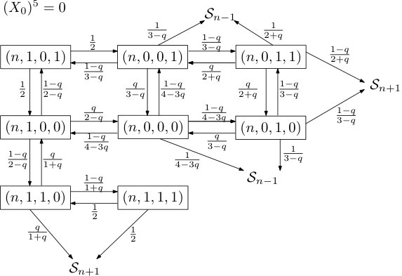 Figure 1
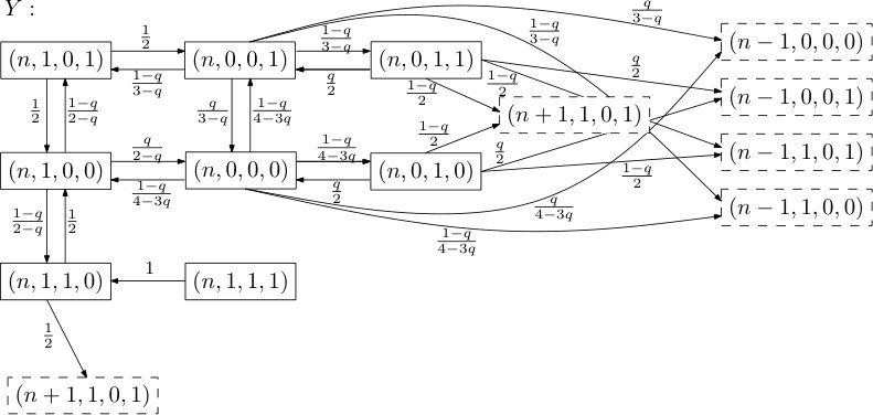 Figure 2
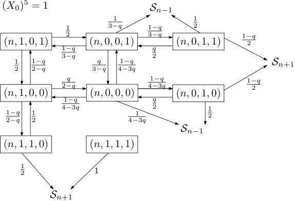 Figure 3
Peer Reviews
No public reviews on file for this paper yet. If you reviewed it on a platform where reviews are public (OpenReview, ICLR, NeurIPS, ICML), you can paste yours below so the community can read it here.
Videos
No videos yet. Explain this paper in a talk, walkthrough, or lecture? Add one.
Taxonomy
TopicsStochastic processes and statistical mechanics · Diffusion and Search Dynamics · Material Dynamics and Properties
Phase transition for a non-attractive infection process in heterogeneous environment
Marinus Gottschau
TUM School of Management and Department of Mathematics, Technische Universität München, Arcisstraße 21, 80333 München, Germany
,
Markus Heydenreich
,
Kilian Matzke
Mathematisches Institut, Ludwig-Maximilians-Universität München, Theresienstraße 39, 80333 München, Germany
[email protected], [email protected]
and
Cristina Toninelli
CNRS, Laboratoire de Probabilités et Modèles Aléatoires, Univ. Paris VI et VII, Bâtiment Sophie Germain, Case courrier 7012, 75205 Paris Cedex 13, France
Abstract.
We consider a non-attractive three state contact process on and prove that there exists a regime of survival as well as a regime of extinction. In more detail, the process can be regarded as an infection process in a dynamic environment, where non-infected sites are either healthy or passive. Infected sites can recover only if they have a healthy site nearby, whereas non-infected sites may become infected only if there is no healthy and at least one infected site nearby. The transition probabilities are governed by a global parameter : for large , the infection dies out, and for small enough , we observe its survival. The result is obtained by a coupling to a discrete time Markov chain, using its drift properties in the respective regimes.
Key words and phrases:
Contact process, phase transition, survival versus extinction
2010 Mathematics Subject Classification:
82C22, 82C26
C.Toninelli acknowledges the support by the ERC Starting Grant 680275 MALIG and ANR-15-CE40-0020-03
1. Introduction
1.1. History
The classical contact process, as introduced by Harris in 1974 [10], has been a central topic of research in interacting particle systems. It is formally defined as -valued spin system, where 1’s flip to 0’s at rate 1, and flips from 0 to 1 occur at rate times the number of neighbors in state 1, where is a parameter of the model. Commonly, the lattice sites are called ‘individuals’, which are either infected (i.e., in state 1) or healthy (i.e., in state 0). Many fundamental questions have been settled for this model, the results are summarized in the monographs by Liggett and Durrett in [7, 12, 13].
Among the most important results are the existence of a phase transition for survival of a single infected particle, the complete convergence theorem, and extinction of the critical contact process. Much more refined results have appeared in recent years. In view of these successes, it may seem surprising that results are considerably sparse as soon as multitype contact processes are considered. Results have only be achieved in very specific situations, examples are the articles by Cox and Schinazi [4], Durrett and Neuhauser [5], Durrett and Swindle [6], Konno et al. [11], Neuhauser [14], and Remenik [15] for various models.
Our focus here is on the contact process with three types, and this carries already severe complications. A fair number of models considered in the literature stems from a biological context (either evolvement of biological species or vegetation models); typical questions that have been considered are coexistence versus extinction and phase transitions. Examples are the work of Broman [3] and Remenik [15].
There are two features that are shared by all of these models: they are monotonic and they are (self-)dual (we refer to [13] for a definition of these terms). These two properties are crucial ingredients in the analysis; if they fail, then most of the known tools fail. This might be illustrated by looking at Model A in [1], which is a certain 3-type contact process. Even though there are positive rates for transitions between the various states of this model and apparent monotonicity, the lack of any usable duality relation prevented all efforts in proving convergence to equilibrium for that model.
For the model considered in the present paper, it appears that there is no duality relation that we can exploit and monotonicity is restricted to a very particular situation only. Yet we are able to prove the occurrence of a phase transition by means of coupling to certain discrete-time Markov chains and analyzing drift properties of these chains. We believe that the technique presented here is useful in greater generality. A motivation for studying this process stems from the connection with the out of equilibrium dynamics of kinetically constrained models, as we will explain in detail in Section 1.3. We believe that the proof techniques apply in similar situations.
1.2. The model
Our state space is , equipped with the product topology (which makes compact). Further, is a parameter and is a Markov process on . We say that at time ,
[TABLE]
Informally, we can describe the process as follows. Each site independently waits an exponential time with intensity 1 and then updates its state according to the following rules:
- •
If at least one neighboring site is healthy, then becomes healthy with probability and passive w.p. .
- •
If at least one neighbor is infected and none is healthy, then a previously healthy becomes infected w.p. , a previously passive becomes infected w.p. and remains in its state otherwise.
For a more formal description, the process can be characterized by its probability generator, which is the closure of the operator
[TABLE]
[TABLE]
Here, and . Furthermore, is the configuration where for all and , .
For an initial configuration , we denote by the corresponding probability measure. This superscript will be dropped for the sake of convenience if context permits.
As we wrote earlier, monotonicity is an important tool in the analysis of such processes. One monotonicity property the process exhibits is the following.
Claim 1**.**
For arbitrary and , we have that
[TABLE]
where and .
In words, additional infected sites cannot decrease the chance of the infection’s survival. However, the same is not necessarily true anymore for and .
Proof.
If we couple the two processes with respective initial measures, we claim that, almost surely, for all and . This is a consequence of the definition of the dynamics and corresponding transition rates. ∎
1.3. Results and discussion
Our main result is a phase transition for in the parameter : if is very close to [math], then any number of initially infected sites survives with positive probability, whereas if is close to , then the infection dies out with probability .
Theorem 2**.**
There exist values such that
- (i)
for any initial configuration , we have
[TABLE] 2. (ii)
and for any initial configuration with , we have
[TABLE]
We thus prove the existence of different regimes without relying on duality properties. Since there is no monotonicity that can be exploited here, we can not rule out that there are more than one transitions between the regimes “the infection dies out” and “the infection survives”. However, we conjecture the following statement to be true.
Conjecture**.**
The function is decreasing in .
This would imply a critical value such that if the infection survives with positive probability, while if the infection dies out with probability .
Note that the case is degenerate and of little interest, as it admits traps: If there is a site and a time such that we exhibit , then this triple will remain fixed for all .
A very related process to the one just introduced is the simpler version for which, informally, the second condition is altered to: “If at least one neighbor of is infected and none is healthy, then becomes infected.” It is clear that the set of infected sites in this version dominates our process. However, the same proof techniques used below yield similar results to Theorem 2 (namely, also a phase transition).
Connections to kinetically constrained models.
This model has an indirect connection with Frederickson-Andersen 1 spin facilitated model (FA1f) [2, 8, 9]. In this case, the configuration space is and the dynamics are defined as follows: a site with occupation variable [math] flips to at rate iff at least one among its nearest neighbors is in state zero; a site with occupation variable flips to [math] at rate iff at least one among its nearest neighbors is in state zero. Note that the constraint for the and the updates are the same and the dynamics satisfies detailed balance w.r.t. the product measure with . Note also that the dynamics of our contact process coincide with the FA1f dynamics if we start from a configuration which does not contain infected sites.
A non trivial problem for FA1f dynamics is to determine convergence to the equilibrium measure for some reasonable initial measure, e.g. an initial product measure with density of healthy sites different from [2]. We will now explain how our results provide an alternative approach to prove convergence to equilibrium in a restricted density regime. A possible strategy to prove convergence to equilibrium for FA1f dynamics started from an initial configuration is to couple it with some distributed according to . This gives rise to a process with 4 states . Here, [math] represent sites where both configurations are [math]; sites where both configurations are ; sites where is [math] and is 1; and sites where is and is [math]. If we now denote the union of sites in state and as ”infected sites”, then if infection dies out, the original process started in is distributed with the equilibrium measure (since there are no more discrepancies with the process evolved from which is at equilibrium at any time). It is not difficult to verify that the dynamics of the state contact process induced by the standard coupling among two configurations evolving with FA1f dynamics are such that the union of sites in state and is dominated by the infected sites of our -state contact process. Thus when infection dies out for our process it also dies out for the -state contact process and from our Theorem 2 (ii) we get convergence to equilibrium for for the FA1f dynamics. This result was already proven by a completely different technique in Blondel et al. [2] for parameter . Notice that convergence to equilibrium is expected to hold for FA1f dynamics at all starting from satisfying the hypothesis of our Theorem 2 (ii), namely infection should always disappear in the state contact process. This is certainly not the case for our state contact process which has a survival extinction transition, as proved by Theorem 2 (i).
2. The small regime
In this section, we prove assertion (i) of Theorem 2. First, We define
[TABLE]
the set of configurations where infected sites form a finite, nonempty interval.
Proposition 3**.**
Consider some . Then there exists such that
[TABLE]
For the proof, we observe first that the set of sites in state 2, which we call the infected cluster, is always connected. We would like to focus on the behavior of the infected boundary sites and so, due to symmetry, on
[TABLE]
the position of the rightmost infected site. If there is only one infected site (thus, leftmost and rightmost infected site coincide), both with positive probability the next change in number of infected sites might result in zero (extinction of the infection) or two infected sites. If the number of infected sites is at least two, only the status on the sites to the right of the rightmost infected site have direct influence on the ‘movement’ of .
In (an informal) summary, if the infection shrinks to size one, it recovers with positive probability to size at least two. If we show that from there, infection spreads with positive probability, we obtain our result. Therefore, we focus on this latter regime in the following.
With this in mind, we now introduce a Markov chain, which can be interpreted as a simplified model of the rightmost infected site and its local right neighborhood, and prove a drift property for it. This shall turn out to be useful when coupling this auxiliary Markov chain to our original process in section 2.2.
2.1. An auxiliary Markov chain
We define a Markov chain living in the (countable) state space . We denote its first coordinate as the chain’s level or state and thus can partition into its -states
[TABLE]
for any integer . The Markov chain is defined by its transition graph shown in Figure 1. The subgraphs induced by are isomorphic, and furthermore, two states from and for have transition probability zero. Hence, for simplicity, we can restrict ourselves to depicting the transition graph induced by , with additional states in along with their respective transition probabilities. We denote the probability measure of this Markov chain by (we trust that this causes no confusion with the measure of the interacting particle system).
We define the stopping time to be the first time the Markov chain changes its level:
[TABLE]
Using (for ) to access the th component of the state which is in at time , say that is a progressive step (progress) if and similarly call a regressive step (regress) if . We say that a natural number is a step time (step) if is either a progressive or a regressive step.
Lemma 4**.**
Let and . Then there exists such that
[TABLE]
for all .
Proof.
The proof proceeds by counting paths in the transition graph. We define
[TABLE]
We also set to be the weight of the 2-cycle between states and . The weight of a cycle is the probability that the Markov chain transitions along this cycle in the transition graph. As a path may use this cycle arbitrarily often, we have
[TABLE]
using the strong Markov property. This leads to the explicit lower bounds
[TABLE]
For small , all of these values are strictly larger than , except for , where we have as . Finally set to be the weight of a 2-cycle between states and and observe that, by counting paths ending in , we have
[TABLE]
In the first parenthesis, the first term comes from paths ending in and , whereas the second terms comes from paths ending in as well as . The lemma follows for sufficiently small.
∎
Lemma 5**.**
There exists such that for all , we have
[TABLE]
Proof.
We start by defining
[TABLE]
to be the first level change after and actually prove . Noting that after two level changes, will either have increased or decreased by 2 or not changed at all, the lemma follows from proving
[TABLE]
for any integer . To this end, we make the following observation, which is an immediate consequence of the definition of the Markov chain dynamics.
Observation 1**.**
Let . Then from , it follows that . On the other hand, if , then , with probability , is one of the two states and, with probability , is one of the two states .
We can thus restrict ourselves to proving (1) for being one of the two ‘good’ -states , as we are allowed to choose sufficiently small. Combining Observation 1 with Lemma 4, we have
[TABLE]
for some and appropriately small. Recalling that was the weight of a 2-cycle between states and and the value of a 2-cycle between states and , and setting , as well as , we have
[TABLE]
with the bound obtained simply by counting paths from to which pass through in their second to last step. With small enough ( say), we are now able to bound , the probability of double regress from , as follows:
[TABLE]
Rearranging by defining and and observing that the event implies that , we continue to find that
[TABLE]
for our chosen and sufficiently small, where have been defined in the proof of Lemma 4. Note that again we make heavy use of the strong Markov property as well as the bounds from Lemma 4. ∎
2.2. The coupling
We are now ready to return to our process. Recall that should be thought of as a model of the right neighborhood of the rightmost infected site in the original process. Intuitively speaking, we want to find a coupling such that at any given time—this, however, is ill-defined. To make it more precise, let us first formally build towards the discrete version of the segment of the process that is of interest (i.e., the right neighborhood of the rightmost infected site). For a realization of the process in , we define the map as
[TABLE]
Hence, is the segment of the process we are interested in. Let be the sequence of clock rings for site . That is, and for all . This allows us to define , the sequence of times of clock rings of the process restricted to , as and
[TABLE]
for all . We are interested in the process , a subset of , where and
[TABLE]
for all . In words, is the embedded discrete time chain of , and is the chain obtained from by removing all of the self-loops. Process is the one which, in certain time windows, behaves very much like . To make this precise, we define with and
[TABLE]
to be the times when either the position of the rightmost infected particle changes or the clock at the site determining the boundary condition, , rings. We call the stable windows for all . A stable window closes whenever the boundary site rings or the infected site moves. We can now proceed to describe the behavior of in a stable window. As we did for , we can partition the state space of into its levels and, as no confusion arises this way, call them as well. The dynamics within depend only on , namely the initial state also encoding the boundary conditions, and are therefore Markovian. Given this initial state for , we can depict the transition graph in a very similar way as the one for , as the subgraphs induced by the levels are again isomorphic, the states in neighboring levels are terminal as they ‘close’ the window . Conditional on the boundary conditions, the two transition graphs are shown in Figures 2 and 3.
Lemma 6**.**
We have that for any
[TABLE]
for any integer . In words, conditioned on closing due to a level change, the probability of progress in is bounded from below by the probability of progress in .
Proof.
Knowing that does not change its fifth coordinate (its boundary conditions as a clock ring would close the window) within allows us to couple the first four coordinates of with while considering both cases of ’s boundary conditions and aim for the desired domination. It is not hard to see that dominates under passive boundary conditions: Note that the transition probabilities as well as the states one ends up in after regress are the same except for state , which only slows the progress of .
Let us justify why the same holds for healthy boundary conditions by showing that for any path leading to progress in , we can find a union of heavier paths in (with those unions being disjoint). It is clear that for all and any progressive path in last visiting , we can find a heavier one in using the edges between states and .
Next, observe that for with healthy boundary conditions, we have additional edges between states and . So any path in leading to progress and last visiting either one of these two states may make use of these edges and then progress in . Defining to be the weight of a 2-cycle between these states we have that, starting from state ,
[TABLE]
so these extra paths add up precisely to the weight of the edges from to . An analogous computation gives the same result when starting from state . ∎
Proof of Proposition 3.
Lemma 6 is valid regardless of the boundary condition, so we can glue together stable windows until the event is satisfied—that is, until a window ends with a level change. In this case, there are two possibilities, namely (progress) or (regress).
In the canonical coupling of the first four coordinates of and within , we obtain that after regress, and end up in the same state (w.r.t. to the first four coordinates of ), whereas after progress, is in one of the states or (with determining the new boundary condition), while will find itself in . So in any case, is in a state from which progress in less likely.
In summary, Lemma 5 shows that dominates a random walk on with positive drift and so has a positive drift. Due to the coupling obtained from Lemma 6, this drift carries over to . Hence, the law or large number for a random walk with drift yields the claimed statement. Finally, Theorem 2 (i) follows from Proposition 3 via Claim 1. ∎
3. Extinction for large
We import some notation from Section 2. Namely, let be the discrete time process describing the rightmost infected site and its neighbors and let denote all -levels of its state space. Similar to how and were defined for the Markov chain in that section, we define for as
[TABLE]
where we set , to be the sequence of level changes of . We abbreviate when it is convenient. We next define two stopping times describing the length of consecutive progressive and regressive steps, respectively. That is, we set
[TABLE]
and call a progressive and a regressive interval, respectively. It is clear that we can partition into alternating progressive and regressive intervals. Our aim is to prove that the length of a progressive interval is, in expectation, less than the length of a regressive one. Note that if is a regressive step, then for some integer , where
[TABLE]
Similarly, if is a progressive step, then for some , with
[TABLE]
The following lemma is the main step in the proof of Theorem 2 (ii).
Lemma 7**.**
In the above notation, we have that
[TABLE]
for und sufficiently large.
Proof of Theorem 2 (ii).
As observed above, starting at , any progressive interval must start from a state, whereas any regressive interval must start from a state. Hence, the conditioning in Lemma 7 is not a restriction and the rightmost infected site is dominated by a -valued random walk with negative drift, which yields the claimed result.
∎
Turning towards the proof of Lemma 7, a key observation is the fact that, when is sufficiently large, healthy sites drift towards each other. More precisely, given a connected set of passive sites with healthy boundary conditions, we expect the size of this set to decrease with time. With this in mind we define
[TABLE]
for some and , i.e. the distance of to the next healthy site in .
Lemma 8**.**
Let . Given any initial distribution taking values in . Assume that for some site . Then for the process with , we have
[TABLE]
Proof.
Let be state of the process at time [math]. Due to translation invariance and symmetry, we shall consider site and assume the closest healthy site is located at for all times . Since we are only interested in an upper bound, we always assume that . In doing this, we obtain a process whose -value dominates the original one. We thus end up with the following simplification:
- •
If site updates, then with probability , it becomes passive and ,
- •
if site updates, then with probability , it becomes healthy and ,
and those are the only updates changing the position of . Hence, the expected change of after an update is . The number of updates in of these two sites is -distributed, and with probability , an update yields a change of position, so , the number of position changes in , is -distributed. Hence, as all of this remains true for , the statement follows by Wald’s lemma. ∎
Note that Lemma 8 is very much in the spirit of Proposition 4.1 in [2], even though we need a much weaker statement to prove Lemma 7, namely that is not increasing.
Proof of Lemma 7.
We begin by considering and noting that, no matter the boundary conditions,
[TABLE]
In words, following a regressive step, we witness another regressive step with probability at least . That is because from , ends up in another regressive step within three steps or less, regardless of a change of boundary conditions during that time. As a direct consequence, gets arbitrarily large for . On the other hand, we have that there exists such that
[TABLE]
for all not too small ( say), and thus
[TABLE]
So if we can bound the last quantity by some constant, we are done. This is where Lemma 8 comes in. We bound this expectation by “jumping” to the closest healthy site, infecting all passive sites on the way. More precisely, we progress the infection by force until reaching a state in .
[TABLE]
which is bounded by a constant, combining Lemma 8 with the fact that the second term goes to [math] as . ∎
The reference list from the paper itself. Each links out to its DOI / PubMed record.
- 1[1] J. van den Berg, J.E. Björnberg, and M. Heydenreich, Sharpness versus robustness of the percolation transition in 2d contact processes. , Stochastic Process. Appl. 125 (2015), no. 2, 513–537.
- 2[2] O. Blondel, N. Cancrini, F. Martinelli, C. Roberto, and C. Toninelli, Fredrickson-Andersen one spin facilitated model out of equilibrium , Markov Process. Related Fields 19 (2013), no. 3, 383–406. MR 3156958
- 3[3] E. I. Broman, Stochastic domination for a hidden Markov chain with applications to the contact process in a randomly evolving environment , Ann. Probab. 35 (2007), no. 6, 2263–2293. MR 2353388 (2009 a:60118)
- 4[4] J. T. Cox and R. B Schinazi, Survival and coexistence for a multitype contact process , Ann. Probab. 37 (2009), no. 3, 853–876.
- 5[5] R. Durrett and C. Neuhauser, Coexistence results for some competition models , Ann. Appl. Probab. 7 (1997), no. 1, 10–45. MR 1428748 (98g:60178)
- 6[6] R. Durrett and G. Swindle, Are there bushes in a forest? , Stochastic Process. Appl. 37 (1991), no. 1, 19–31.
- 7[7] Richard Durrett, Lecture notes on particle systems and percolation , The Wadsworth & Brooks/Cole Statistics/Probability Series, Wadsworth & Brooks/Cole Advanced Books & Software, Pacific Grove, CA, 1988. MR 940469
- 8[8] Glenn H. Fredrickson and Hans C. Andersen, Kinetic Ising model of the glass transition , Phys. Rev. Lett. 53 (1984), 1244–1247.