Exotic matter on singular divisors in F-theory
Denis Klevers, David R. Morrison, Nikhil Raghuram, Washington Taylor

TL;DR
This paper investigates exotic matter representations on singular divisors in F-theory, providing a framework for their analysis and explicit models, revealing new insights into geometric constraints and the swampland.
Contribution
It introduces a general method for analyzing exotic matter in F-theory on singular divisors, including explicit descriptions for symmetric representations and their algebraic structures.
Findings
Explicit models for symmetric matter representations in F-theory.
Identification of geometric constraints affecting low-energy spectra.
Examples of theories in the swampland with no F-theory realization.
Abstract
We analyze exotic matter representations that arise on singular seven-brane configurations in F-theory. We develop a general framework for analyzing such representations, and work out explicit descriptions for models with matter in the 2-index and 3-index symmetric representations of SU() and SU(2) respectively, associated with double and triple point singularities in the seven-brane locus. These matter representations are associated with Weierstrass models whose discriminants vanish to high order thanks to nontrivial cancellations possible only in the presence of a non-UFD algebraic structure. This structure can be described using the normalization of the ring of intrinsic local functions on a singular divisor. We consider the connection between geometric constraints on singular curves and corresponding constraints on the low-energy spectrum of 6D theories, identifying some new…
Click any figure to enlarge with its caption.
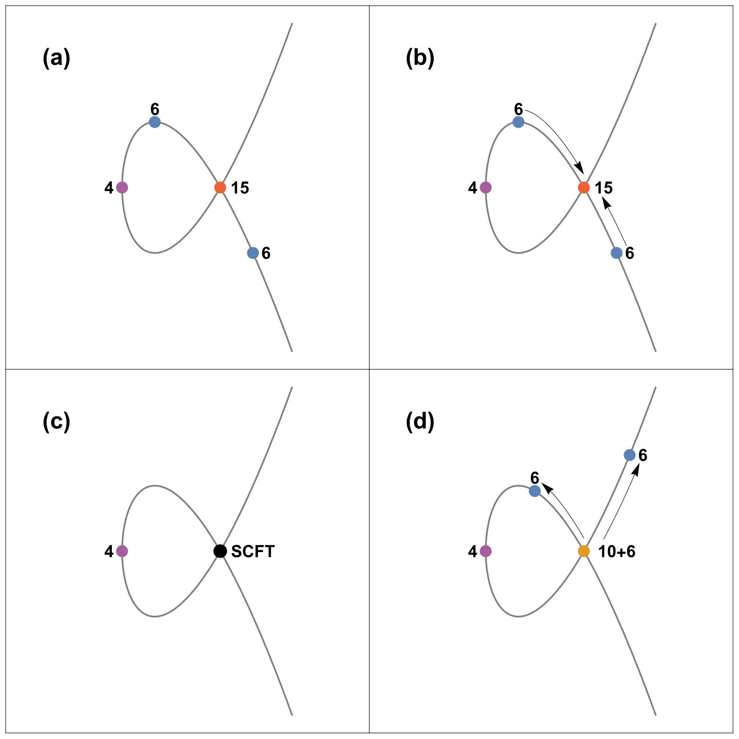 Figure 1
| Representation | Dimension | ||||
| 1 [] | 0 | [] | 0 | ||
| 4 | 0 | 8 | 1 | ||
| 10 [5] | 0 | 41 | 6 [3] | ||
| 20 | 0 | 136 | 21 |
| Base | ||
|---|---|---|
| Number of Tensors | 0 | 1 |
| Divisor Class of Curve | ||
| Genus | ||
| Multiplicity | ||
| Adjoint Multiplicity | ||
| Fundamental Multiplicity | ||
| Singlet Multiplicity |
| Representation | Dimension | ||||
|---|---|---|---|---|---|
| 6 | 0 | 9 | 1 | ||
| 1 | 0 | 0 | |||
| 5 | 0 | 1 | |||
| 15 | 0 | 7 |
| Parameter | Homology Class |
|---|---|
| SU(3)-rep | Multiplicity | Fiber | Locus |
|---|---|---|---|
| SU(4)-rep | Multiplicity | Fiber | Locus |
|---|---|---|---|
| Parameter | Homology Class | Equivalent Symbol in [11] |
|---|---|---|
| SU(2)-rep | Multiplicity | Fiber | Locus |
|---|---|---|---|
Peer Reviews
No public reviews on file for this paper yet. If you reviewed it on a platform where reviews are public (OpenReview, ICLR, NeurIPS, ICML), you can paste yours below so the community can read it here.
Videos
No videos yet. Explain this paper in a talk, walkthrough, or lecture? Add one.
Exotic matter on singular divisors in F-theory
Denis Klevers
David R. Morrison
Nikhil Raghuram
and
Washington Taylor
Abstract
We analyze exotic matter representations that arise on singular seven-brane configurations in F-theory. We develop a general framework for analyzing such representations, and work out explicit descriptions for models with matter in the 2-index and 3-index symmetric representations of SU() and SU(2) respectively, associated with double and triple point singularities in the seven-brane locus. These matter representations are associated with Weierstrass models whose discriminants vanish to high order thanks to nontrivial cancellations possible only in the presence of a non-UFD algebraic structure. This structure can be described using the normalization of the ring of intrinsic local functions on a singular divisor. We consider the connection between geometric constraints on singular curves and corresponding constraints on the low-energy spectrum of 6D theories, identifying some new examples of apparent “swampland” theories that cannot be realized in F-theory but have no apparent low-energy inconsistency.
1 Introduction
The relationship between geometric structure and the physical content of quantum field theories and gravity theories has been a theme in string theory and related research for several decades. The formulation of F-theory [1, 2, 3] has given perhaps the most general geometric approach yet to the construction of physical theories with varied gauge groups and matter content. While the F-theory “dictionary” that relates geometry and gauge symmetry is well understood both mathematically and physically, the corresponding connection between geometric structure and the representation theory content of matter fields is still under development. In this paper we analyze some new aspects of the geometry-matter F-theory correspondence, associated with nonperturbative features of singular seven-brane configurations that carry exotic matter representations in the associated physical picture.
In standard perturbative type II string theory, a stack of D-branes carries a U() gauge symmetry, and only certain relatively simple matter representations can arise. In particular, on supersymmetric branes in flat space, intersecting branes carrying U() and U() gauge groups give rise to bifundamental and matter fields. The two-index nature of the matter fields in perturbative type II constructions comes from the realization of these matter fields through strings, where the Chan-Paton factors on the two ends of the string correspond to the two indices on the matter fields. In the nonperturbative framework of F-theory, the range of matter fields that can be realized is much broader. In F-theory compactifications where an SU() gauge group is realized (e.g. via a type Kodaira singular fiber) over a smooth 7-brane locus, the generic types of matter that arise are adjoint (), fundamental (), and two-index antisymmetric () matter fields. These correspond again to two-index representations with origins common to those in the perturbative formulation of the theory. Another set of matter fields that can arise in F-theory are the 3-index antisymmetric representations (20, 35, 56) of SU(6), SU(7), and SU(8), which can arise through nonperturbative F-theory constructions over a smooth seven-brane locus [4, 5, 6, 7]. These antisymmetric representations can be realized explicitly through relatively standard Weierstrass models in F-theory.
A more exotic set of SU() representations in F-theory are those for which the Young diagram has more than one column, corresponding to some indices over which the representation is symmetric. Such representations can only arise over seven-brane configurations that are singular [8]. The possibility of a two-index symmetric representation arising at a double point singularity was suggested by Sadov [9], and considered further in [5], but can only be distinguished from an adjoint through global geometric considerations. Explicit examples of such two-index symmetric representations of SU(3) were found and explored in [10, 7]. These explicit models exhibit rather subtle structure in the Weierstrass model involving a nontrivial cancellation in the ring of functions on the divisor carrying the gauge group, which depends crucially on the structure of the singularity. Similar explicit representations of 3-index symmetric representations of SU(2) were found in [11] to have a related structure. In this paper we develop a systematic approach to understanding these kinds of representations, using the non-UFD (UFD = unique factorization domain) nature of the ring of functions on singular seven-brane loci.
The structure of this paper is as follows: In §2 we review some basic relevant background on F-theory constructions and low-energy 6D supergravity theories. Most of the explicit examples in the paper are given in the context of 6D models, where the understanding is most complete, though the same principles will apply for 4D F-theory models. In §3 we give two very simple examples of the kinds of construction needed to realize exotic non-UFD matter realizations, to illustrate the general structure of these models. In §4 we give a concise description of the mathematical framework needed to describe the Weierstrass models for these kinds of constructions. In §5 we go into detail in analyzing the general construction of models with two-index symmetric matter at double points, and in §6 we describe the construction of models with three-index symmetric matter at triple points. In §7 we show how these geometric constructions are connected to more standard matter constructions through “matter transitions” analogous to those studied in [7]. We then in §8 consider how the configurations that contain these exotic matter fields are constrained both in F-theory and from low-energy considerations, and identify cases where the F-theory constraints are stronger than those that are known in the low-energy theory, giving some new examples of theories in the 6D supergravity “swampland”. In §9 we consider the more general question of what exotic matter representations are allowed in any F-theory models, and conclude that those studied here seem to essentially exhaust the interesting possibilities for matter charged under nonabelian gauge groups, though some more complicated representations are not ruled out from low-energy considerations and currently lie in the swampland. §10 contains some concluding remarks.
2 Background on F-theory and 6D supergravity
We review here very briefly some basics of F-theory and summarize the important features of the 6D supergravity theories that are the focus of the explicit examples in this paper. Further background on F-theory can be found in [1, 2, 3] or in the review notes [12, 13].
2.1 SU() gauge factors in F-theory
We will consider F-theory models on a base , defined by a Weierstrass model
[TABLE]
Here are functions depending on local coordinates in that define an elliptic curve at each point in . More formally, these are sections of line bundles , , where is the canonical class of the base; this fixes the total space of the elliptic fibration over to be an elliptic Calabi-Yau manifold. The elliptic fibration is singular along the seven-brane locus defined by the discriminant
[TABLE]
We will focus here primarily on type Kodaira singularities, which locally are like perturbative stacks of D7-branes. Such a singularity occurs when the discriminant vanishes to order in a local coordinate . In a local expansion in ,
[TABLE]
To realize an SU(2) gauge symmetry along , we must then have . For vanishing at order 0, we have , which can be satisfied if for some . For vanishing at order 1 we then have , which can be solved by . This gives a local construction of the Weierstrass model with an SU(2) gauge symmetry over the locus .
This analysis is extended to higher order in in [5]. To get an SU(3) gauge group, there are several conditions. First, the “split” condition states that must be a perfect square . Second, the vanishing of at order 2 gives the further conditions that for some function and that .
One of the principal goals of this paper is to generalize this kind of analysis to situations where the SU() gauge group is realized on a general divisor that can have singularities. In such a situation the local coordinate is replaced by the section , where the equation defines the divisor .111Thus, is a Cartier divisor. We assume in this paper that the base is nonsingular, which implies that all divisors are Cartier divisors.
2.2 Anomaly cancellation conditions and SU() spectra
In a 6D supergravity theory there are strong consistency conditions on the massless spectrum from anomaly constraints [14, 15]. Using the notation and formalism of [16], the gauge and gauge-gravitational anomaly cancellation conditions can in general be written as
[TABLE]
Here are Green-Schwarz coefficients that live in a lattice of signature and are group theory coefficients defined in e.g. [17], while is the number of matter (hypermultiplet) fields in the representation . There is also the gravitational anomaly constraint
[TABLE]
where is the number of tensor multiplets, is the number of vector multiplets, and is the total number of hypermultiplets. In a model that comes from F-theory, represents the divisor class of the seven-brane curve carrying the gauge group and is the canonical class of . In this case, the genus of the curve satisfies . We can take this more generally as the definition of a quantity in the low-energy theory for any choice of , and an associated simple gauge factor satisfying the anomaly conditions.
For the explicit models in this paper we focus primarily on theories with gauge group SU(2) and SU(3). For each of these gauge groups there is no quartic invariant, so and (2.6) is satisfied automatically. Furthermore, for each of these groups global anomaly conditions constrain and to be integers. We discuss models with each of these gauge groups in turn, and then briefly describe the story for SU() for general .
The anomaly coefficients for are given in Table 1. If we assume that the only representations that arise are the fundamental, adjoint, and 3-index symmetric, then Equations (2.5) and (2.7) can be solved to find:
[TABLE]
The gravitational anomaly constraint then gives
[TABLE]
These are the spectra for the models we wish to describe explicitly here through F-theory by explicit Weierstrass constructions. The multiplicities for such tunings on the simplest base surfaces and are given in Table 2.
One way of understanding the spectrum (2.9) is to note that the most generic model (having the largest number of uncharged scalar fields) with given in most cases corresponds to the model, with adjoint representations and fundamental representations. Because there are only two independent anomaly coefficients , the contribution of any other representation can be described in terms of the fundamental and adjoint, giving an anomaly equivalence [5, 6] such as
[TABLE]
This means that, at least as far as anomalies are concerned, 3 adjoints and 7 uncharged scalars can be exchanged for a half hypermultiplet in the 3-index symmetric () representation and 7 fundamental fields. In [7], it was shown that -index antisymmetric matter representations of SU() that are anomaly equivalent to simpler matter fields can be connected explicitly to more generic fields through unusual “matter transitions” in which the gauge group and tensor content stay unchanged but the matter representations change. In §7 we show that in a similar fashion the transition (2.11) can be realized explicitly as a continuous phase transition between distinct Weierstrass models. Note that for some choices of there are no allowed models with . For example, if in a model with tensor multiplets, then the number of fundamentals being nonnegative implies that there are at least 3-index symmetric representations in any valid model. Such examples have been encountered in [11, 18] and are discussed further in §8.2.
Note that there is also an anomaly equivalence in the low-energy theory
[TABLE]
From this we can see that there are low-energy 6D supergravity models that contain 4-index symmetric representations of SU(2) that satisfy all the anomaly constraints including the gravitational anomaly [8]. For example, the generic model with has 21 adjoints, 64 fundamental representations, and 82 uncharged scalars. This is anomaly-equivalent to a model with 128 fundamentals, a single 5 and 12 uncharged scalars. As discussed further in §9, we do not believe however that this model has an F-theory realization.
A similar story holds for SU(3) models. The anomaly coefficients of the simplest representations are given in Table 3. A generic model has adjoints and fundamental representations. There is an anomaly equivalence for every SU(), that relates an adjoint (plus an uncharged scalar) to a combination of symmetric and antisymmetric two-index tensors
[TABLE]
This enables the exchange of adjoints and symmetric matter while maintaining the total value of , to which each contributes one. For SU(3), the two-index antisymmetric representation is equivalent to the antifundamental, so this simply gives a fundamental hypermultiplet, and the anomaly equivalence is . Note that there are anomaly-consistent SU(3) spectra with choices of that must have two-index symmetric representations. For example, for at the generic model has 28 adjoint fields and 0 fundamentals. At , there is an anomaly-allowed model with 6 adjoints and 30 ’s, along with 45 uncharged scalar fields. There are no fundamentals, however, so despite the anomaly equivalence the ’s cannot be exchanged for adjoints. We return to these models in §8.1.2.
The story is similar for SU(), except that there are three independent representations since generically . Generic models will have adjoints, fundamental matter fields, and two-index antisymmetric matter fields. Adjoints can then be exchanged for symmetric plus antisymmetric fields through (2.13). Finally, note that there is an anomaly equivalence for SU(3) representations in the low-energy theory , so there are anomaly-consistent low-energy models with a three-index symmetric tensor () representation, such as the model with 3 adjoints, 81 fundamentals, one 3-index symmetric, and 56 uncharged scalar fields. Again, we argue in §9 that such models cannot be realized in F-theory.
This completes the overview of the low-energy theories that we encounter in the various constructions later in this paper. Before moving on, we note that the anomaly equations suggest that, at least for 6D theories, gravity cannot be decoupled if certain representations are present. If a representation has a larger than , Equation (2.7) implies that must be positive if there are any hypermultiplets in the representation . (If half-hypermultiplets are possible, this scenario occurs when .) Recall that the Green-Schwarz coefficients live in a lattice of signature . The negative part of the signature corresponds to tensors living in tensor multiplets, whereas the positive part corresponds to the tensor living in the graviton multiplet. A positive indicates that the tensor field in the graviton multiplet participates non-trivially in the Green-Schwarz mechanism. Thus, if gravity is decoupled, one cannot cancel anomalies if there are any representations with (or for representations with half-hypermultiplets). The representation of has a that leads to positive , as do the of and the of . While these representations occur in known 6D supergravity theories coming from F-theory, they cannot be part of a 6D theory without gravity, explaining their absence from the classification in [19]. The representation of and the representation of , both of which we believe cannot be realized in F-theory, also have . It may be interesting to further explore whether this fact gives new physical insights into these representations.
3 Tuning with a non-UFD ring: examples
Before getting into technical details, to give a sense of the spirit of the constructions needed we give a pair of simple examples of how nontrivial cancellations can arise in the Weierstrass models realizing and singularities when the divisor supporting the gauge group is itself singular. We take to be a section of the line bundle associated with , so that in local coordinates denotes the locus of points in .
3.1 Triple points and SU() 3-symmetric matter
As a simplest example, we want to tune on . Here , , and are some functions (sections) that do not admit any factorization. In general, cannot be factorized and defines a divisor that is singular at the locus of points . For example, if , and are respectively irreducible quadratic, linear, and cubic functions in some local coordinates, then gives a pair of triple point singularities. The general idea is that we want to expand the ring of functions on to allow to be factorized. Formally this is done using the mathematical notion of the normalized intrinsic ring, which is developed in detail in the following section. More informally, the idea is that to generalize the expansions (2.3, 2.4) for instead of , the coefficients must be in the natural ring of functions on . The auxiliary function from §2.1, however, can be in a larger ring that is given by adjoining an element such that ; note that solves the cubic equation . This gives the normalized intrinsic ring for , which has somewhat the flavor of a Galois field extension. For the cubic we choose an element , the analogue of ,222We have changed the symbol to agree with the notation used later: parameters that are well-defined only in the normalized intrinsic ring are capitalized and have a tilde. to be the following element of the normalized intrinsic ring
[TABLE]
We can then define the leading terms of and in terms of
[TABLE]
and note that they are restrictions of functions on the F-theory base, as indicated by the righthand side of the above expressions. We then have
[TABLE]
We thus have a nontrivial cancellation in the discriminant made possible by the form of . At the next order we have
[TABLE]
This can be made to vanish by taking, for example, for some . Then . We then have the expansion
[TABLE]
This gives an SU(2) on the divisor , which has triple points at the loci in a nonstandard Weierstrass form.
3.2 Double points and SU() symmetric matter
Now consider SU(3) with a double point associated with
[TABLE]
Again, the normalized intrinsic ring is given by adjoining such that ; this time, we have , which solves the quadratic equation . Working in the normalized intrinsic ring, we have proportional to and proportional to , but because the split condition must be enforced to obtain , we must take . As a possible solution not in standard form, we choose in the normalized intrinsic ring, so that
[TABLE]
is well-defined in the ring of functions on .
At leading order, . Cancelling we have
[TABLE]
At the next order, we have
[TABLE]
so we wish to solve
[TABLE]
in the normalized intrinsic ring. Since , for any solution we must be able to write
[TABLE]
where is in the normalized intrinsic ring. We then take
[TABLE]
The challenge is to ensure that and lie in the appropriate ring of functions on .
If we choose then and we have
[TABLE]
ensuring gauge symmetry.
4 Mathematical description of the normalized intrinsic ring
Let us review the history of how our understanding of the singular fibers in F-theory fibrations has evolved over time. The first step was Kodaira’s classification [20], which related specific geometric singular fibers to specific choices of monodromy on the homology of elliptic curves along loops in the base surrounding the singular fiber. (In F-theory terms, this classifies singular fibers according to the ways in which they source the scalar field in type IIB supergravity [21].) The total space of the corresponding Weierstrass model has an ADE singularity, and this – together with the known gauge theory behavior for perturbative IIB 7-branes – allowed the association of a gauge algebra to each codimension one singularity (for eight-dimensional theories). A straightforward method to “read off” the type of Kodaira singular fiber from a Weierstrass equation is also known, in terms of the orders of vanishing of the Weierstrass coefficients and as well as the discriminant .
The second step was the realization that in lower dimensional compactifications, another kind of monodromy comes into play: monodromy could act as automorphisms of the Kodaira singular fibers themselves [22]. We refer to this as “Tate monodromy” to distinguish it from the original “Kodaira monodromy” because Tate’s algorithm [23] (a refinement of the Kodaira classification) allows one to fully classify gauge algebras in lower dimension, including monodromy considerations.333From Tate’s point of view, this arises because the function field of the F-theory base is not algebraically closed. This was spelled out in [4], with some clarifications in [6].
Tate’s algorithm also allows one to “read off” the matter content from certain codimension two singular loci, but it was realized in [5] and [24] that the analysis from [4] was not complete, and that analysis was reexamined in those two papers.444Ref. [5] had the goal of describing as many matter configurations as possible, whereas Ref. [24] was devoted to exploring to what extent the original Tate algorithm was predictive in codimension two. The term “Tate form” has come to mean a model whose gauge algebra is determined by an equation in one of the forms studied in [4, 24]; the goal of this paper is to begin a systematic study of models that are not in Tate form.
The key technique in both [5] and [24] was to find expansions for the Weierstrass coefficients and as finite power series in , when defines a component of the discriminant locus of the fibration. More precisely, sequences of functions , , …, and , , …, were found such that
[TABLE]
and satisfying other properties that clarify the structure of the corresponding singularities. Each function or is chosen for its properties as an intrinsic function on . That is, if we introduce the algebraic coordinate ring555This algebraic coordinate ring need only contain functions defined in a neighborhood of the point being studied, and for example might take the form for appropriate local coordinates and . of (an open subset of) the F-theory base with , then the key properties of these functions are determined by their images in . We can think of as the ring of intrinsic local functions on .666A note about terminology: every affine algebraic variety has an associated “coordinate ring;” this applies equally well to open subsets of the F-theory base and as well as to open subsets of the divisor on . This terminology can be confusing when more than one algebraic variety is under discussion, so we shall use the word “intrinsic” to emphasize that the functions in question need only be defined on the divisor .
In both [5] and [24], a condition was imposed that this ring of intrinsic local functions on should be a unique factorization domain (UFD), and that property was used extensively in analyzing the expansion. In this paper, we will go beyond that assumption, and consider divisors whose ring of intrinsic local functions is not a UFD.
A fundamental result in algebraic geometry says that any algebraic variety has a “normalization” that is nonsingular in codimension one. (If has dimension one, then is in fact nonsingular.) The functions on are described by the “normalization” of the ring . We shall refer to this normalization as the normalized intrinsic ring.
A key property that holds when has dimension one is that the normalized intrinsic ring is a UFD. This means that, at least for 6D theories, we will be able to use aspects of the UFD analysis from [5] but applied to elements of the normalized intrinsic ring rather than elements of the intrinsic ring itself. For all divisors studied in this paper (of whatever dimension), we will assume that the normalized intrinsic ring is a UFD.
Algebraically, the normalized intrinsic ring is what is known as the “integral closure of in its field of fractions.” Algorithms are known for computing this normalization in very general settings: we refer the reader to Chapter 1 of [25] for a very readable account of this. In this paper, we will focus on examples that are closely connected to interesting matter representations in F-theory.
We begin with a simple example of a normalized intrinsic ring: a cusp singularity on . That is, we assume that has a local equation of the form . The corresponding intrinsic ring takes the form
[TABLE]
and is visibly not a UFD, since in that ring.
The algebraic prescription for finding the normalized intrinsic ring is to add elements in the field of fractions of that satisfy a monic polynomial with coefficients in . (In general it may be necessary to shrink the open set in order to find such elements, and the systematic algorithm can be complicated: see [25].) In this particular case, we only need to adjoin the element , which satisfies two equations:
[TABLE]
That is, we have
[TABLE]
which can be rewritten in the form since can be eliminated using and then can be eliminated using .
The geometric interpretation is this: the function is well-defined away from the cusp and has a well-defined limit on the smooth divisor , so it should be added to the ring of functions. Note that adding this function resolves the UFD issue, since in the larger ring.
This structure now gives us some additional flexibility in building F-theory models. For to be contained in the discriminant locus, we need to be identically zero. If the ring of intrinsic functions is itself a UFD, this implies that there is a function such that777We are following the normalization used in [5]. and . In the case of a cusp singularity, although the ring of intrinsic functions is not a UFD, the normalized intrinsic ring is a UFD. We will get a solution to the problem of putting into the discriminant locus if we can find a function with the property that and both lie in the subring of functions coming by restriction from the F-theory base. Choosing satisfies this property without itself being the restriction of a function from . Thus, we can take and to obtain a solution.
This is a gratifying result, since one of the first observations one makes about F-theory in dimension six or lower is that the multiplicity one part of the discriminant almost always contains cusp singularities, at points where and both vanish. Here we see this arising from a local analysis in a non-UFD case. While in this situation the discriminant generically does not support a gauge group and there is no charged matter, the non-UFD structure here is a simple example of the kind of thing that we encounter in the cases here with matter at double point and triple point singularities.
The examples in §3 were also phrased in terms of the normalized intrinsic ring. We will be more systematic about the structure of that ring in subsequent sections. We will also use a notation aimed at distinguishing between elements of the various rings. Variables that are well-defined only in the normalized intrinsic ring are capitalized and marked with a tilde. For the most part, variables that are in either the coordinate ring or the ring of intrinsic local functions are lowercase; the main exceptions are the discriminant and variables related to it (such as terms in a power series expansion of ).
5 Detailed analyses of constructions: double points
In this section, we describe how to derive more general tunings using the normalized intrinsic ring techniques. Specifically, we focus on tuning on curves of the form
[TABLE]
with symmetric matter localized at the double points. The previously derived models with symmetric matter use curves that can be written in this form, making this case an important one to consider. Before performing the tuning, we describe some of the physical and conceptual ideas behind the tuning. These conceptual insights in fact foreshadow some of the features of the Weierstrass model. We then give the algebraic derivation of the tuning and discuss the resulting matter spectrum. The final tunings are also given in Appendix A.
The quantities , , , , and are all elements of the coordinate ring of the F-theory base. However, for some purposes it is convenient to work with (5.1) more abstractly, and to do computations in an auxiliary ring and to regard as an element of that ring.
5.1 Geometry, monodromy and symmetric matter
In field theory, one can Higgs an gauge group to by giving a VEV to an antisymmetric hypermultiplet. The corresponding branching rules for the representations are
[TABLE]
From §2.2, there are anomaly-equivalent matter spectra related by the exchange
[TABLE]
The branching rules in (5.2) imply that both sides of (5.3) branch to the same representations. In other words, two anomaly-equivalent models Higgs down to the same model, even though the two models initially have different matter spectra. A similar story holds for . Giving a VEV to two fundamental hypermultiplets Higgses down to , with the branching rules given by
[TABLE]
There are anomaly equivalent spectra related by the exchange
[TABLE]
Again, both sides of the exchange branch to the same representations, implying that the anomaly-equivalent models Higgs down to the same model.
An F-theory model with symmetric matter should have a non-UFD Weierstrass tuning. This follows for from the fact that a UFD Weierstrass tuning always has a Tate description [24] and has only the generic fundamental, adjoint, and two-index antisymmetric matter representations. After Higgsing, the model contains no exotic matter and would presumably not require non-UFD structure. Therefore, the Weierstrass model deformation corresponding to the Higgsing process should remove non-UFD structure. If we know the specifics of the deformation, we may be able to guess where non-UFD structure appears in the tuning.
Fortunately, the Higgsing process is part of the well-known story of the split condition. In six and fewer dimensions, the singularity type of a codimension-one singularity may not fully specify the gauge group. Suppose the discriminant vanishes to order along some codimension-one locus , while and do not vanish along the locus. The resulting gauge group can be either or . To distinguish between the two possibilities, one must consider Tate monodromy. When one goes around a closed loop in the gauge divisor, exceptional curves in the resolved fiber may or may not be interchanged. If no interchange occurs, the gauge group is ; otherwise, the gauge group is . At the level of the Weierstrass model, information about the monodromy is encoded in the split condition, namely, whether there exists defined on such that
[TABLE]
Essentially, the condition asks whether is a perfect square along . If the condition is satisfied, the gauge group is ; otherwise, monodromy effects are present, and the gauge group is .
When is even, the standard UFD tunings for and are identical except for the split condition. From the arguments above, any non-UFD structure in the model with symmetrics must disappear after Higgsing. Therefore, non-UFD structure can only appear at the level of the split condition when is even. The split condition is evaluated only on , so one needs to consider only the leading terms and in and . In both the UFD and non-UFD tunings, and will respectively be proportional to and , and will be proportional to . For the UFD case, the only way to satisfy the split condition is for to be a perfect square. The non-UFD case allows for more possibilities. If , the choice satisfies the split condition on , as
[TABLE]
These observations suggest the form that the non-UFD tunings should take. For even , one starts with the non-split UFD tuning and implements the split condition in a non-UFD fashion. Importantly, all of the discriminant cancellations occur exactly, and all of the non-UFD structure is contained in the split condition. For odd , there are minor differences between the split and non-split UFD tunings, so the prescription for the non-UFD tunings is more complicated. Nevertheless, the odd tunings implement that split condition in a non-UFD fashion, and there are only relatively minor changes from the UFD tuning. In the remainder of this section, we show via direct calculation that these insights hold in the tunings and tunings. The explicit formulas for higher are described in §5.4.5.
This picture also explains from a geometric perspective why the non-UFD tunings give the symmetric matter representation. As described in [5], the difference between the adjoint and the symmetric + antisymmetric matter representations at a double point of a divisor supporting an singularity comes from the two distinct ways in which the two copies of associated with the gauge factors on the two branches of the divisor are embedded into the Dynkin diagram associated with ’s in the resolution of the singularity in the total space of the fibration over the double point. When is a perfect square, so lives in the ring of intrinsic local functions as in the UFD case, this embedding gives the adjoint representation of SU(N). When, on the other hand, lives only in the normalized intrinsic ring , which is a quadratic extension of , there is a change of sign between the two branches of the divisor that intersect at the double point, which flips the orientation of one of the Dynkin diagrams relative to the other, giving the symmetric + antisymmetric representations of SU(N). An example of how this works is given explicitly in Appendix C.
5.2 Generators of the normalized intrinsic ring
To find the generators that must be added to the ring of intrinsic local functions in order to obtain the normalized intrinsic ring, it is helpful to rewrite the expression (5.1) in the more suggestive form
[TABLE]
Thus, in the field of fractions we have two expressions for a single element :
[TABLE]
Moreover, we can see that
[TABLE]
so that satisfies the monic polynomial in
[TABLE]
If denotes the ring of intrinsic local functions, then the normalized intrinsic ring is888We have actually only established that is an element of this ring, not that it is the only element that needs to be added. However, that will be true if everything else about and the elements , is sufficiently general.
[TABLE]
Note that
[TABLE]
so that vanishes in , as expected. Note also that is the discriminant of the quadratic (5.1) considered as a function of . Thus, extending the ring by is closely related to the natural extension by the root of the quadratic . Using , however, gives a particularly simple and clear way to understand the algebraic structure of the models. Our discussion of triple points in §6 takes a similar form.
5.3 Monomials and polynomials in the normalized intrinsic ring
To perform the Weierstrass tunings, we need to determine when a product of polynomials in lies in . It is helpful to first focus on individual monomials before turning to polynomials. Consider a monomial in of the form . Monomials for which is even are automatically in , as are monomials with . Thus, the only monomials potentially not in are those with , where is odd. Given a monomial with odd , we can repeatedly convert factors to until we are left with a single factor of . Therefore, all monomials in that do not lie in can be written as times an expression in .
A generic polynomial in thus takes the form
[TABLE]
where and are polynomials in . We will be interested in situations where has at least one term that is not proportional to either or . This condition in turn implies that is not in , as will be necessary for a non-Tate Weierstrass tuning.
We now consider the product of two polynomials
[TABLE]
To ensure that this product lies in , we need to be a linear combination of and . The general solution to this999Assuming that all polynomials are sufficiently general: see footnote 8. takes the form
[TABLE]
where and are parts of and which are not divisible by or (which implies that and both lie in ). We would then have that
[TABLE]
which we see lies in after canceling the terms. Note that if then must be [math].
5.4 Tuning process
We start by expanding and as
[TABLE]
In other words, we find an algebraic function101010Ideally, this would be a polynomial in some projective or affine coordinate ring, in practice it may be easier to treat it as a rational function in some situations. such that is divisible by , and then an algebraic function such that is divisible by , and so on. The functions and are not unique, and in fact may not exist on the entire base: they might only exist in open subsets [24].
For any choice of such an expansion, the discriminant can be expanded as
[TABLE]
Although the and are not unique, their images in the quotient ring have important properties which are independent of choices.
5.4.1 Tuning
For the singularity, we require that
[TABLE]
Thanks to unique factorization in the normalized intrinsic ring, there must exist an element in that ring such that
[TABLE]
In principle, might not be well-defined as an element of . However, if we write then having both and in implies that is in (since by the argument above only contains terms proportional to ), so that (and hence ) is a combination of and . That in turn implies that itself lies in . We can therefore solve (5.21) with , i.e., we can choose an algebraic function that solves (5.21) (mod ) and then define
[TABLE]
With such a choice, the zeroth order term of the discriminant vanishes exactly:
[TABLE]
This may naively seem to imply that and lack any non-Tate structure. There is a remaining condition yet to be implemented, however: the split condition. Since our focus is on tuning gauge groups with , we must satisfy the split condition by letting
[TABLE]
Here, is an element of , while must be an element of . From the discussion in §5.3, can therefore be written as
[TABLE]
with , , and all algebraic functions in . is now given by
[TABLE]
5.4.2 Tuning
The discriminant now reads
[TABLE]
To remove the order one term, we simply let
[TABLE]
The order one term of now vanishes exactly, leaving an singularity on the locus .
5.4.3 Tuning to obtain
is now given by
[TABLE]
To tune an singularity and obtain an model, we must have that
[TABLE]
Working in , we have the condition
[TABLE]
The UFD nature of implies that we should tune and as
[TABLE]
where .
Of course, the expressions for and should be well-defined in . To ensure Equation (5.32) is consistent with this requirement, should be expanded as
[TABLE]
From the analysis of §5.3, and can now be written as
[TABLE]
and
[TABLE]
After these expressions are plugged in, Equation (5.29) takes the form
[TABLE]
We will refer to one-sixteenth of the quantity in square brackets as . is proportional to , and we have an singularity and an gauge group. Importantly, this is the first step with non-trivial cancellations in the discriminant.
Before proceeding to higher orders, let us summarize the model. The Weierstrass model is described by
[TABLE]
with , , and given respectively by Equations (5.26), (5.34), and (5.35). Full, expanded expressions for and are given in Appendix A. The homology classes of the parameters are given in Table 4. For some choices of , , , and , certain parameters may have ineffective homology classes. It might be possible to obtain a valid model in such situations by setting the ineffective parameters to zero. In many cases, setting a parameter to zero has only benign effects, giving a valid model. For example, if is set to zero, the model does not change significantly and is free of problems. Other cases may lead to an invalid model, however. There are situations in which and are ineffective and are forced to be zero; then vanish to orders at the loci. Meanwhile, if , , , , and are all set to zero, the discriminant vanishes exactly. The effectiveness of the various parameters therefore constrains the set of possible models. In particular, this Weierstrass tuning cannot realize certain matter spectra, as discussed further in §8.1.
Table 4 also gives the map from the model considered here to the two previous models with symmetric matter [10, 7]. In order to obtain either of the two previous models, one of the parameters, either or , must be set to a constant. This restriction suggests that both of the previous models are in fact specializations of the model derived here. In particular, setting a parameter to a constant forces a relationship between the three unspecified homology classes in Table 4. If is set to as in [10], the homology class of the curve is fixed:
[TABLE]
Likewise, forcing to be a constant, as in [7] leads to the constraint that
[TABLE]
As a result, the two previous models have only two unspecified homology classes, and the model given here has an extra degree of freedom. The extra unspecified homology class is important physically, as it allows for matter spectra not possible with the previous two models. Making a parameter constant also affects matter transitions that exchange adjoints for symmetric matter, as discussed in §7.
5.4.4 Tuning to obtain
For the discriminant to be proportional to , we require that
[TABLE]
Working in and using (5.21), (5.28), and (5.32), this condition can be written as
[TABLE]
We therefore need to be proportional to , which can be accomplished by letting
[TABLE]
for some (i.e., we are solving (5.42) in , not in ). With these redefinitions, is now zero, and (5.41) is now
[TABLE]
We thus redefine as
[TABLE]
is now proportional to , and we have an singularity. Note that in this discussion since is untuned, we could in principle set to vanish by setting , but we have left the appearances of explicit for clarity.
To summarize the model, the and for the Weierstrass model are given by
[TABLE]
with given by Equation (5.26). The homology classes for the parameters are given in Table 5. As before, ineffective parameters should be set to zero, which may lead to an invalid model.
The tuning is essentially a UFD non-split tuning with a specialized non-UFD tuning for . As mentioned in §5.1, this result matches the expectation that, for symmetric representations, the only non-UFD structure should appear when implementing the split condition.
5.4.5 Tuning higher
The tunings for larger symmetries with symmetric matter follow from the general principles described in §5.1. In fact, the procedure requires only small modifications of the known UFD tunings. Note that we only discuss models with fundamental, two-index antisymmetric, adjoint, and two-index symmetric matter; the strategies we discuss may not apply to situations with three-index antisymmetric matter, for example. The tuning for even is less complicated than the odd tuning, so we first focus on the even case.
An gauge group with symmetric matter can be Higgsed down to an model without any singular higher-genus matter. For the , we therefore start with the UFD tuning for a non-split singularity tuned on the curve . As discussed in [5], this tuning takes the form111111Note that, for clarity, we have used different variables and notations than [5].
[TABLE]
with
[TABLE]
We now specify that has the quadratic form given in (5.1). To enhance the gauge symmetry to , we must perform further tunings to satisfy the split condition. In the UFD case, this is accomplished by letting . But for the non-UFD situation we are interested in here, we use instead of , where is an element of as in Equation (5.25). therefore takes the form of Equation (5.26):
[TABLE]
The split condition is satisfied and the gauge symmetry is enhanced to . The double points at now contribute symmetric matter.
For the tunings, we start with the UFD tuning of a split singularity, which is also given in [5]:
[TABLE]
with
[TABLE]
We assume that the singularity is tuned on a curve as in Equation (5.1). To convert the UFD model to one with symmetric matter, we consider and , elements of that are expanded as
[TABLE]
We then replace , , and with the well-defined expressions for , , and in :
[TABLE]
The replacements give an model in which both the discriminant cancellations and the split condition involve non-Tate structure.
5.5 The matter spectrum
Finally, we determine the structure of codimension two singularities and the associated matter spectrum of F-theory models with gauge symmetry from Kodaira singularities over divisors with double point singularities. We explicitly analyze the resulting matter spectrum for SU(3) and SU(4), while our general techniques are readily applicable to SU(N) for general .
We will focus in the following on two-dimensional base manifolds of the elliptic fibration corresponding to 6D F-theory models. While in principle the matter spectrum for 6D models is essentially determined by anomaly constraints once the symmetric matter content is known, for the non-Tate models constructed here explicitly identifying the structure of the algebra-geometric loci and multiplicity of the matter fields is much more subtle than in the simpler case of the UFD-based constructions. We note that the results obtained for the matter representations and the homology class of their corresponding codimension two loci in are the same for F-theory compactifications to 4D with three-dimensional base manifolds ; in fact, following the analysis of [26], in much of the discussion here we use a language more appropriate for four dimensions, where each matter type is associated with an irreducible codimension two locus.
5.5.1 General comments
We begin with some general facts and observations on the determination of the matter loci and spectrum in F-theory models that is common to both examples discussed in the following. We recall that in general the matter content of F-theory (except for adjoint matter) is encoded in the singularities of the elliptic fibration at codimension two in the base . The variety in defined in this way is in general reducible with each of its irreducible components yielding a particular enhancement of the singularity type of the elliptic fibration, which corresponds to a particular matter representation. Each matter representation can, in principle, occur on multiple irreducible components, and all of those representations must be collected together to describe the entire matter content of the model. Note that for compactifications to 6D there are typically many such components for each representation (since irreducible components are points), while for compactifications to 4D each representation might be associated to only one irreducible component.121212But note that even in this case, it is possible for there to be more than one component associated to a given matter representation.
More explicitly, in the examples at hand, we have two types of codimension two singularities. We have a factorization of the discriminant as
[TABLE]
with and singular at .131313The case is special as there is no codimension one singularity giving rise to gauge symmetry, despite the appearance of a codimension two symmetry of type .
- •
The first type of codimension two singularities are the common zeros at codimension two in of . These contain the conventional matter representations of SU(N), i.e. the fundamental representation and, for , also the two-index anti-symmetric tensor representation of SU(N).
- •
Second, there are codimension two singularities from the singularities at of . The discriminant vanishes to order at these loci. They support the two-index symmetric tensor representations of SU(N). In general, singularities of this type could also support localized adjoint matter, as discussed in more detail in §7; we assume in the analysis here that we have a non-UFD Weierstrass model where all the double point singularities in the discriminant locus support symmetric matter through the kind of mechanism analyzed explicitly in Appendix C.
From a technical perspective, the determination of the irreducible components of the codimension two loci described by the ideal is the most challenging. In simple situations, such as local analyses with being a normal coordinate to a smooth divisor, which is assumed for example in the standard analysis of Tate forms, can simply be inserted into . In particular, in the UFD-based analysis of [5], the structure of clearly decomposes into a contribution from corresponding to antisymmetric matter fields, and a residual discriminant component capturing the fundamental matter fields. However, in the situation at hand, with given by (5.1), we can not solve globally. This poses a problem if we want to compute the homology classes of the codimension two matter loci. One way to circumvent this problem is introduced in [26] to which we refer for further details. There, a general primary decomposition of the locus is performed, yielding its associated prime ideals, each of which corresponds to an irreducible component of the codimension two singularities of the elliptic fibration. Then, one determines the homology class of each of these irreducible components using their respective prime ideals. (If we can, it is desirable to only partially decompose the prime ideal, grouping various irreducible components together when they correspond to the same matter representation.)
Note that part of the challenge in identifying the irreducible components of the codimension two locus arises from the non-UFD structure of the ring of intrinsic local functions. We could in principle analyze the codimension two structure in the normalized intrinsic ring, in which we could write e.g. . Since the vanishing locus of is the same as that of , and the latter is in the ring of intrinsic local functions, we can identify in a fairly direct fashion the geometric locus of vanishing , which will support fundamental matter. In the analysis of this section, however, we work more generally in the geometry of the ring of intrinsic local functions, which will in principle automatically handle issues such as multiplicity. These analyses should agree; the results of this section should in part be interpreted as a confirmation of the structure of the matter spectrum that can be derived more directly through anomaly analysis or other approaches.
We now outline the procedure described above in the context of the two F-theory models with SU(3) and SU(4) gauge symmetry.
5.5.2 Matter spectrum of SU(3) models
We consider the F-theory model with singularity over the divisor defined in (5.1). It is specified by the non-Tate Weierstrass form in (5.37) with the tunings (5.34) and (5.35). We refer to Appendix A for a concise summary of the Weierstrass model. The discriminant, given by Equation (A.7), is proportional to , so that we have in our notation from (5.56)
[TABLE]
For the convenience of the reader, we begin by summarizing the findings of the determination of matter content based on the analysis of codimension two singularities of this model along with the corresponding 6D matter content of F-theory in Table 6. Note that in the absence of exotic (symmetric) matter, these multiplicities can be understood directly from the UFD Weierstrass expansion in e.g. [5], where the discriminant takes the form and fundamental matter arises at the zeros of , which is in the class since . This direct interpretation is more difficult to make, however, in the more intricate non-UFD models we have constructed here, as discussed above, although from the point of view of the “matter transitions” described in §7 the multiplicities in this table can also be reproduced by starting with a UFD construction and trading adjoint matter for symmetric matter through matter transitions.
We begin with the discussion of the adjoint as well as the matter localized at the singularities of . As pointed out in [9, 5], both representations arise from the arithmetic genus of the curve . Decomposing the genus of into its geometric genus and contributions from the double point singularities, we obtain
[TABLE]
Here we employ that a double point contributes to the arithmetic genus , which we compute via adjunction in the second equality. As has been shown in [27], there are hypermultiplets in the adjoint where is the geometric genus of the curve, i.e., the genus of its normalization. As discussed above, we assume that we have a construction where all double points correspond to the two-index symmetric tensor of SU(3). For the constructions of this paper, this follows from the geometric logic described earlier, is confirmed in §7 via a matter transition argument, and is shown explicitly through resolution in an example in Appendix C. Thus, we identify the intersection number as the multiplicity of matter fields in the representation , and we arrive at the matter multiplicities in the first and second lines in Table 6.
We note that each double point contributes also one hypermultiplet in the of SU(3) as noticed in [10]. There this was shown by Higgsing the model to an Abelian model with two U(1)’s. The presence of an additional can be motivated by viewing the double points locally as the collision of two different 7-branes carrying an SU(3) gauge group; the intersection points support matter in the bi-fundamental representation .141414It is the non-trivial point of our analysis that the relevant representation is and not . As the two 7-branes are really part of one single brane in the global geometry, we have to identify them and view the bi-fundamental as the reducible representation , which exhibits the group theory decomposition in the non-Tate situation where a symmetric matter representation is present.
Next we turn to the conventional matter localized at the intersection loci . We first gain some intuition about the possible matter loci by solving locally and away from its double point singularities and inserting the solution into . We immediately observe a factorization of into two components, which indicates the existence of two irreducible varieties inside .
In order to find the varieties inside which correspond to different types of matter, we make a computation in the auxiliary ring . We have performed a rigorous primary decomposition of in that ring using Singular [28], obtaining two prime ideals denoted by and . (Note that these ideals are prime in although they may factor further once specific elements of the ring are chosen to represent the variables in the auxiliary ring. For compactifications to 6D, they will almost certainly factor further since each codimension two prime ideal is supported at a single point of the F-theory base.)
Explicitly, we find
[TABLE]
where we have to quotient by the ideals
[TABLE]
in order to obtain a prime ideal. The prime ideal is too lengthy to be reproduced here; it is generated by several large polynomials in the parameters in and . It can be obtained by computing the saturation of the ideal w.r.t. the ideal , i.e. the repeated quotient ideal
[TABLE]
Next we analyze the singularity type of the elliptic fibration along the varieties , defined by the vanishing loci of , inside the variety . By investigation of the orders of vanishing of , we find that
[TABLE]
which indicates Kodaira singularities of type and respectively [20, 23]. This means that the variety supports matter in the fundamental of SU(3) [4], whereas is the locus of a degeneration of an singularity to type . This does not correspond to the emergence of additional physical degrees of freedom due to the lack of new holomorphic curves to be wrapped by M2-branes.
Finally, for the computation of the matter multiplicity of fundamentals, we need to know the homology class of . As we are on a two-dimensional base , the variety is just a collection of points and its homology class is simply the number of such points. We start by computing the multiplicities of , inside . Using the resultant technique discussed in [26], we find the multiplicities to be and , respectively, i.e. we obtain the following relation in homology:
[TABLE]
The homology class of the left hand side of this equation is readily computed using the explicit expression for in (5.1) and in (5.40). We then compute using its definition (5.59) as being contained in a complete intersection among the additional components specified by the complete intersection ideals in (5.60). The homology classes of the latter are easily computed noting their definition as irreducible complete intersections. Their multiplicities inside the complete intersection in (5.59) are computed using the resultant as and , respectively. Thus, we obtain
[TABLE]
where we used the homology classes of all relevant sections given in Table 4. The first term in the first equality is the homology class of the complete intersection in (5.59) and the second and third terms are the homology classes of the varieties corresponding to the ideals in (5.60). Putting everything together, we obtain the homology class of using the homology relation (5.63) as
[TABLE]
The first term in the first equality is the homology class of and the second term is (5.64). We also double check the result for by directly working with the lengthy ideal , i.e. by finding a suitable complete intersection containing among with other “auxiliary” varieties given as complete intersections. We then just have to compute the homology class of the complete intersection and subtract the homology classes of the auxiliary varieties with their appropriate multiplicities inside , which we compute using the resultant.
In summary, we obtain the contribution (5.65) from Kodaira singularities of type over the component inside to the multiplicity of matter fields. As noted earlier, there are additional matter fields in the representation for each ordinary double point singularity [10]. The combined results leads to the full matter multiplicity in the last line of Table 6.
We conclude by checking the consistency of the derived SU(3) matter spectrum by testing anomaly freedom of the 6D theory. Following the discussion of §2.2, we identify and . We then see that anomaly cancellation follows immediately for the spectrum in Table 6 upon the identification , .
5.5.3 Matter spectrum of SU(4) models
Next, we consider an F-theory model with SU(4) gauge algebra arising from a Kodaira singularity of type over the divisor defined in (5.1). The non-Tate Weierstrass form is given in (5.45) with a discriminant as in (5.56) of the form
[TABLE]
with given in (A.10) in Appendix A. We again first summarize the matter content of the 6D F-theory in Table 7.
As in the previous discussion of SU(3), the adjoint matter arises from the geometric genus given by the general formula (5.58) while the symmetric matter arises from the double point singularities on . Thus, we arrive at the matter multiplicities in the first and third lines in Table 7.
We note that, as in the SU(3) case, each double point contributes also one hypermultiplet in the of SU(4), which we can understand by decomposing the bi-fundamental as at the double points.
Next, we discuss the emergence of conventional matter localized at the intersection loci . Performing a primary decomposition in the auxiliary ring , we immediately obtain two prime ideals denoted by and corresponding to two irreducible varieties inside . Explicitly, we find
[TABLE]
where we have to quotient by the ideals
[TABLE]
in order to obtain a prime ideal, as in (5.59). The prime ideal is once again too lengthy to be reproduced here. It can be obtained by computing the saturation of the ideal w.r.t. the ideal , or as the quotient ideal
[TABLE]
The singularity type of the elliptic fibration along the two varieties , is readily analyzed by investigation of the orders of vanishing of . They are given by
[TABLE]
respectively, indicating Kodaira singularities of type and respectively [20, 23]. This means that the variety supports matter in the fundamental of SU(4), indicated by a local enhancement to SU(5), while the variety , in contrast to the SU() case with , supports matter in the anti-symmetric representation , indicated by the enhancement to SO. We note that this is completely analogous to the SU(5) case discussed, for example, in great detail in [29].
Finally, the matter multiplicities of fundamentals and require the knowledge of the homology classes of and . The multiplicities of , inside are computed with the resultant technique of [26] to be and , respectively, resulting in the homology relation
[TABLE]
The homology class of the complete intersection on the left hand side is readily computed using the explicit expression for in (5.1) and in (A.10). We then cross-check our computations for and using their respective definitions (5.69) and (5.67). Indeed, we find
[TABLE]
and
[TABLE]
which obey this consistency check. Here we used the homology classes of all relevant sections given in Table 5. The numerical prefactors in front of the terms that are subtracted are the multiplicities of the redundant components (5.68) and computed using the resultant.
In summary, we obtain that the number of fundamental hypermultiplets is given by (5.72) and the number of hypermultiplets in the contributed from fibers is given by (5.73). Together with the additional matter fields in the representation at each each ordinary double point singularity we obtain the third and last lines of Table 7.
We conclude with the consistency check on the derived SU(4) matter spectrum via 6D anomalies. Following the discussion of §2.2, we again set and . We then see that anomaly cancellation follows immediately for the spectrum in Table 7 upon the identification and .
The upshot of the analysis in this subsection is that we can explicitly determine the loci where the distinct matter representation types are localized, even in the more subtle non-Tate non-UFD cases studied earlier in this section.
6 Detailed analyses of constructions: triple points
In this section, we describe how to derive models with three-index symmetric matter using the normalized intrinsic ring techniques. We focus on tuning the singularity on curves of the form
[TABLE]
with the matter localized at the triple points. This form of the gauge curve agrees with that used in [11]. However, the tuning derived here is more general than the one in [11], even though both models use the same form of the gauge curve. We first describe the normalized intrinsic ring and give an algebraic derivation of the tuning. We then discuss the resulting matter spectrum. The final model is summarized in Appendix B. Note that this construction can also be used to describe tri-fundamental matter fields, by choosing a cubic form that explicitly factorizes. There is a corresponding auxiliary ring in which some of our computations are done.
6.1 Description of the normalized intrinsic ring
Notice that because is a homogeneous polynomial of degree , the equation can be written in the form
[TABLE]
Thus, in the field of fractions of we have two expressions for a single element :
[TABLE]
which leads us to relations and to be used in the normalized intrinsic ring. For ease of notation, we introduce
[TABLE]
so that the relations can be written and .
Furthermore,
[TABLE]
where
[TABLE]
so that is also a relation in the normalized intrinsic ring. In fact, if all parameters are generic, we can define the normalized intrinsic ring as
[TABLE]
We will later need an expression for in this ring, which we derive by writing
[TABLE]
where
[TABLE]
Then
[TABLE]
We denote the right hand side of the previous equation by .
Note that is in the intrinsic local ring , so that we are really only carrying out an extension by a quadratic element of the ring. This construction is parallel to the ring we found in the double point case in §5.
6.2 Tuning process
We start by expanding and as
[TABLE]
just as done in §5.4. The discriminant is then given by
[TABLE]
6.2.1 Tuning
For an singularity, the zeroth order term of the discriminant must be proportional to :
[TABLE]
Because the normalized intrinsic ring is a UFD, there must be some element in such that
[TABLE]
Of course, and must have well defined expressions in , which places restrictions on the form of . We start by expanding as
[TABLE]
where and have well-defined expressions in . Focusing first on , the only potentially problematic term in
[TABLE]
is the term. To ensure that this term lies in , should take the form
[TABLE]
(Note that cannot take this form if we want a non-UFD Weierstrass tuning.)
can then be defined as
[TABLE]
Essentially, we have replaced the terms in involving with the corresponding expressions in . also lies in after the redefinition of , and can now be defined as
[TABLE]
We now have
[TABLE]
and the discriminant is proportional to . has a lengthy expression that we do not give here.
6.2.2 Tuning to obtain
For an singularity, the discriminant must be proportional to , and
[TABLE]
must be proportional to . In other words
[TABLE]
Let us first focus on the term. It is easiest to work with the field of fractions of , in which is equivalent to
[TABLE]
If were allowed to be an element in the field of fractions, we could immediately determine how should be defined to cancel the contributions. But is an element of the coordinate ring, and the terms in Equation (6.25) cannot be fully canceled using . In particular, the and terms in the square brackets are not proportional to and cannot be canceled. To proceed further, and must be tuned so that
[TABLE]
where and are some expressions in the coordinate ring. Considering the situations in which either or leads to the conditions that
[TABLE]
These conditions suggest that and should be defined as
[TABLE]
With these definitions, takes the form
[TABLE]
where all terms above are well defined in . We now define to be
[TABLE]
leaving
[TABLE]
We now turn to the term. Working in , the condition for the singularity is now
[TABLE]
should therefore be identified with
[TABLE]
must lie in , which implies that must take the form
[TABLE]
should in turn be defined as
[TABLE]
With these redefinitions, the discriminant is now proportional to , indicating we have successfully tuned an model. To summarize, and are now given by
[TABLE]
with
[TABLE]
The homology classes of the various parameters are given in Table 8.
Table 8 also gives the dictionary between this model and the previous model given in [11]. The key difference between these models is that is forced to be a constant in [11]. This restricts the homology classes: for to be a constant,
[TABLE]
The model of [11] thus has only two unspecified homology classes, whereas the model derived using the normalized intrinsic ring techniques has three unspecified homology classes. This extra freedom has physical consequences. In particular, the model derived here can support a wider array of matter spectra than the model in [11]. Otherwise, the two models are fairly similar. In fact, if and are set to zero and is set to a constant, the two models are equivalent.
6.3 The matter spectrum
Equipped with the general non-Tate Weierstrass model described by (6.36) through (6.40), we proceed with the determination of the singular locus and corresponding matter spectrum of the corresponding F-theory model. As before, we will focus on two-dimensional base manifolds of the elliptic fibration yielding a 6D supergravity theory, although the following results also carry over to non-chiral F-theory compactifications to 4D. The discussion will be very similar to the one in §5.5.
We recall that the matter content of F-theory (except for the adjoint matter) is encoded in the codimension two singularities of the elliptic fibration specified by the Weierstrass model (6.36)-(6.40). In the case at hand, we have two types of codimension two singularities. First, there are the common zeros at codimension two in of with being defined via . These contain, as we demonstrate below, the conventional matter representations of SU(2), i.e. the representation. Second, there are codimension two singularities from the singularities of at , which support the triple symmetric matter representations of SU(2). As before in §5.5, the determination of the irreducible components of the codimension two loci in is the most challenging, and in general involves performing a primary decomposition following the procedure outlined in [26] to which we refer for further details.
Before going into the details of this computation, we summarize the found matter content based on the analysis of codimension two singularities of the general non-Tate Weierstrass form (6.36)-(6.40) along with the corresponding 6D matter content of F-theory in Table 9.
We begin with the discussion of the non-localized matter, i.e. the adjoint matter, as well as the matter localized at the singularities of . The geometric genus of , which counts adjoints, is given by the arithmetic genus corrected by the contribution from the triple point singularities:
[TABLE]
Here we employ that every triple point contributes to the arithmetic genus , which we compute via adjunction in the second equality. We assume in analogy to the discussion of matter with double point singularities that we are working with a construction in which all the triple points contribute 3-symmetric matter representations. Identifying as the multiplicity of matter fields in the representation , we thus arrive at the matter multiplicities in the first and third lines in Table 9. We note that each triple point contributes only one half-hypermultiplet as the representation is pseudo-real.
Next we turn to the conventional matter localized at the intersection loci . We first gain some intuition about the possible matter loci by solving locally away from its triple point singularities and inserting the solution into . We immediately observe a factorization of into two components, which indicates the existence of two irreducible varieties inside .
Indeed, we can perform a rigorous primary decomposition of in the auxiliary ring using Singular [28] to obtain two prime ideals denoted by and .151515As before, these ideals may factor further once specific elements of the ring are chosen to represent the variables in the auxiliary ring. Explicitly, we find
[TABLE]
where we have to quotient by the ideals
[TABLE]
in order to obtain a prime ideal. The prime ideal is too lengthy to be reproduced here; it is generated by several large polynomials in the parameters in and . It can be obtained by computing the saturation ideal of the ideal w.r.t. the ideal : 161616Due to the complexity of the involved algebra and the limited available computing power, we were only able to determine the ideal in the case where is a random rational number between and .
[TABLE]
Next we analyze the singularity type of the elliptic fibration along the varieties , defined by the vanishing loci of , inside the variety . By investigation of the orders of vanishing of , we find that
[TABLE]
which indicates a singularity of type and respectively [20, 23]. This means that the variety supports matter in the fundamental of SU(2) [4], whereas is the locus of a degeneration of an singularity to ,. This does not correspond to the emergence of additional physical degrees of freedom due to the lack of new holomorphic curves to be wrapped by M2-branes.
Finally, for the computation of the matter multiplicity of doublets, we need to know the multiplicities of , inside . Using the resultant technique discussed in [26], we find the multiplicities to be and , respectively, i.e. we obtain the following relation in homology
[TABLE]
The homology class of the left hand side of this equation is readily computed using the explicit expression for in (6.1) and as it follows from (6.37). We then compute using its definition (6.3) as being contained in a complete intersection among the additional components specified by the ideals in (6.44). The homology classes of the latter are easily computed noting their definition as irreducible complete intersections. Their multiplicities inside the complete intersection in (6.3) is computed using the resultant as and , respectively. Thus, we obtain
[TABLE]
where we used the homology classes of all relevant sections given in Table 8. The first term in the first equality is the homology class of the complete intersection in (6.3) and the second and third terms are the homology classes of the varieties corresponding to the ideals in (6.44). Putting everything together, we obtain the homology class of as
[TABLE]
The first term in the first equality is the homology class of and the second term is (6.48), which has to be subtracted with the correct multiplicity . We also double check the result for by directly working with the lengthy ideal .
We thus obtain the contribution from loci inside to the multiplicity of matter fields as shown in the first term of the fourth line of Table 9. We note that there are additional matter fields in the representation from the ordinary triple point singularities as noted in [11]: group-theoretically, the representation arises in the decomposition at each ordinary triple point of . This shows that each triple point also supports one full hypermultiplet in the representation , which leads to the second contribution in the last line of Table 9.
We conclude by double-checking the derived SU(2) matter spectrum by testing anomaly freedom of the 6D theory. Following the discussion of §2.2, we identify and . We then see that anomaly cancellation follows immediately for the spectrum in Table 9 upon the identification , .
7 Matter transitions
In many situations, the 6D anomaly conditions specify a unique charged matter content given a few parameters. But for the models considered here, these same parameters are not enough to fully determine the matter spectrum, as mentioned in §2.2. Even if , , the gauge group, and the representations are fixed, the 6D anomaly cancellation conditions still admit multiple solutions for the matter multiplicities. Given a particular spectrum, one can find another consistent spectrum through the exchange (2.11)
[TABLE]
The models with meanwhile admit multiple spectra related by the exchanges (2.13)
[TABLE]
The “anomaly equivalent” theories related by the exchanges have the same number of tensor and vector multiplets. From the perspective of the Weierstrass tunings, the homology classes of the various parameters are not fully fixed by the gauge curve homology class and . In turn, there may be multiple charged matter spectra for a given base and gauge curve homology class.
A natural next step is to ask how these anomaly equivalent models fit into the space of vacua. Specifically, is there a process to move between the anomaly equivalent models? As discussed in [7], there are a number of possible ways to connect 6D models. The simplest of these, which can be seen as a purely field-theoretic phenomena, is the Higgs mechanism: there can be a theory with a larger gauge group whose Higgs branch contains both of the models in question. A more exotic type of transition, known since [30, 3], is the tensionless string or small instanton transition in which the number of tensor multiplets in the theory changes. The theory is superconformal at the transition point. A third possibility was raised in [7], where it was shown that anomaly equivalent models for a variety of gauge groups, such as and , are connected by “matter transitions” that occur within the Higgs branch of a superconformal theory. As in the case of a Higgs transition, the original gauge theory must be enhanced, but to a superconformal theory rather than to a theory with larger gauge group. In the context of F-theory, this occurs through a series of tunings and deformations of the Weierstrass model. In field theoretic terms, such transitions relate two theories with the same gauge group and the same number of tensor multiplets via an intermediate superconformal theory which contains both of them in its Higgs branch. The models derived here have similar matter transitions. In addition to being interesting phenomena in their own right, the matter transitions clarify the relationships between exotic higher-genus matter, curve singularities, and non-Tate tuning structures.
Before turning to the matter transitions in specific models, let us first describe how these transitions work in general. The process is illustrated in Figure 1 for . We assume we are working with a 6D F-theory model, although the transitions may occur in 4D models as well. Initially, the F-theory model will have matter located at several codimension two loci. The first step of the transition is to tune the Weierstrass model so that a collection of these loci are moved to a single point. and now vanish to at least orders and at this point, signaling the appearance of a superconformal sector [3, 31, 32]. Next, the Weierstrass model is deformed, separating the superconformal locus again into multiple codimension-two matter loci. The representations supported at these new points are different from those at the beginning of the transition. The SCFT in this example is the “single E-string theory” [33, 34, 30] corresponding to a curve in F-theory. It has a Higgs branch of dimension 29 with a variety of gauge groups and matter representations realized at different points of that Higgs branch.
Overall, the setup can be described in terms of the Higgs branch of a fixed SCFT, within which one finds several distinct loci with a previously selected gauge group, although the matter spectra may differ among the loci. (There are two loci for the example illustrated in Figure 1 below.) The initial tuning moves us from the first locus to the SCFT. One could then, in principle, move onto the tensor branch through a blow-up on the base. Instead, we follow Weierstrass deformations that move us to a new locus within the Higgs branch with the same gauge group but a different matter spectrum. In the simplest cases, the SCFT at the transition point is an E-string theory consisting of a single curve on the tensor branch. The SCFTs for some of the transitions considered here may have extra gauge groups tuned on the curve. However, the simplest transitions do not have additional tensor branch gauge symmetries, suggesting that these gauge groups are not a general requirement for transitions.
Finally, we note a few general observations about the transitions. First, progress through the transition can be described using a single parameter. This may not be immediately obvious from the general discussion or from the detailed analysis of models below. But the transition can be thought of as moving through a single parameter family of models. If desired, one can even write the deformations and tunings explicitly in terms of a single parameter, as done in [7]. Second, the description of the transition process above did not mention introducing or deforming singularities along the gauge curve. This omission is a reflection of an important point regarding singular matter: gauge curve singularities do not automatically contribute exotic matter. In particular, introducing a curve singularity only localizes adjoints at the singular point and does not change the matter content. To make the singular points support exotic matter, the theory must additionally undergo a more dramatic change, such as obtaining a superconformal sector at the transition point. In the examples considered here, the tunings and deformations of the transition that actually change the matter content do not affect the number of singular points along the gauge curve. The elliptic curve singularity type at a double point or triple point may change during the course of the transition. However, the gauge curve singularity is present through the core part of the transition.
7.1 Model with Symmetric Matter
In order to make the discussion more concrete, we first focus on the model with symmetric matter. Recall that if the singularity is tuned on the curve
[TABLE]
the Weierstrass model is described by
[TABLE]
with
[TABLE]
This model admits transitions that cause a net exchange of matter of
[TABLE]
For this discussion, we focus on the transitions that exchange an adjoint and a singlet for . These transitions involve three basic steps described in more detail below:
Introduce a new double point along the gauge curve , localizing adjoint matter at the double point. As mentioned previously, this step does not change the matter content of the theory and thus should not be considered as a core part of the transition. 2. 2.
Further tune the Weierstrass model to obtain an SCFT at the double point. 3. 3.
Deform the Weierstrass model in a different way to remove the SCFT, leading to a model with a different matter spectrum.
The transitions that cause the opposite exchange of matter () can be obtained by inverting the above three steps.
Step 1: Introduce a new double point.
Symmetric matter can occur only at double point singularities along the gauge curve. To convert adjoint matter into symmetric matter, we therefore must first introduce a new double point singularity along the curve. This can be done through the tunings
[TABLE]
, now given by
[TABLE]
has double point singularities at . The tuning introduces a total of double points; in the minimal case, , and there is only one new double point. Note that this tuning does not change the matter spectrum. A double point singularity along an curve can correspond to either or matter [5]. The locus currently supports localized adjoints, as these double points can be deformed away. Thus, while the tunings in (7.9) localize adjoints that previously could propagate throughout the gauge curve, there is no change in the matter spectrum. In other words, one cannot introduce symmetric matter simply by tuning more double points. Changing the matter spectrum requires a more dramatic change, which here entails passing through a superconformal point.
Note that in the description here we have assumed the initial curve has the form (7.3) and already contains some double points. More generally, this need not be the case. An arbitrary smooth curve could be put in this form where so there are no initial double point singularities; in this case, for example, we could tune a single double point singularity from a smooth curve with none by starting with and taking .
Step 2: Move to the SCFT.
Currently, symmetric matter (if present) resides at the locus. To convert the localized adjoints at into symmetric matter, one would like to perform a deformation such as . At this point in the transition, such a deformation is not possible: there are factors of in the Weierstrass model (7.3-7.7) without corresponding factors of . We therefore need to perform the additional tunings
[TABLE]
These tunings make and vanish to orders 4 and 6 at , signaling the presence of an SCFT. In order to produce this superconformal matter, the tuning must have pushed other matter loci to the double points. Prior to the tunings in Equations (7.9) and (7.11), the discriminant takes the form
[TABLE]
where is equivalent to in the normalized intrinsic ring. The discriminant locus contributes fundamentals. After the tunings, vanishes to order 3 on the locus, while vanishes to order 2. Since the locus now supports an SCFT, it should be subtracted out when counting the number of fundamentals after the transition. For each point, fundamentals therefore disappear as a result of the tunings in Equations (7.9) and (7.11). A careful consideration of the available degrees of freedom and redundancies in the Weierstrass model indicates that in the tuning (7.11) two singlets are fixed for each point. This missing matter corresponds exactly to the loci that were pushed to in order to form the SCFT. The effect of this second step can therefore be summarized as
[TABLE]
The SCFT at the transition point is an E-string theory. On the tensor branch, where the singularity is resolved by a blowup on the base, there is a single curve with no additional gauge groups. The gravitational anomaly condition therefore suggests that exactly 29 hypermultiplets should be removed at the transition point in order to produce the SCFT. Indeed, exactly 29 hypermultiplets participate in this step for each point, as seen in the left-hand side of (7.13).
Step 3: Deform the SCFT.
There are now enough factors of in the Weierstrass model to absorb into . However, there will be factors of remaining after such an association. The model at the end of the transition should have the same basic structure as before, suggesting that a tuning with remaining factors of is a specialized model that can be further deformed. To remove the extra factors of , we must perform the deformations
[TABLE]
After this deformation, and are not proportional to . There is no longer an SCFT, as there is no codimension two locus where and vanish to orders 4 and 6. The six fundamentals and two singlets that had disappeared are now restored, and the double points introduced by Equation (7.9) now contribute matter. Every factor of is accompanied by exactly one factor of , so we can now perform the redefinition
[TABLE]
and remove all factors of . The transition is now complete, with a total change of matter of the form
[TABLE]
The net effect of the transition is therefore to exchange for , as expected from the anomaly cancellation conditions. We can also exchange for by inverting the steps in the transition.
The Weierstrass model in fact allows for a second type of transition, although this transition will have the same physical effect. This second transition involves transferring factors into rather than into . To convert adjoints into symmetrics, we initially perform the tunings
[TABLE]
thereby introducing new double points at the loci. The additional tunings
[TABLE]
take us to a superconformal point. The transition is completed with the deformations
[TABLE]
In total, the transition exchanges adjoints for symmetrics through a process identical to that in Equation (7.16). Of course, one can perform the transition in the opposite direction by reverting the steps.
As mentioned in §5.4.3, the previously derived models with symmetric matter are specializations of the ones derived here. In particular, these previous models restrict homology classes by setting certain parameters to constants. These models will not exhibit all of the possible transitions laid out here, but they may still allow some subset of the transitions. For example, the model in [7] essentially forces to be a constant, so transitions where changes are not possible. The transitions where changes, however, are still possible. For the model in [10], is set to one, while both of the transitions considered here change the homology class of . These transitions are therefore not possible in this model. This model has other transitions that connect the different matter spectra, but the theory undergoes more extreme changes during the transition. For instance, when the gauge curve factorizes at the transition point. As a result, the transition point theory has a new gauge group in addition to the SCFT.
Finally, let us examine how non-Tate structure appears as part of the transition. Consider a situation where is initially set to
- There are no double points, so the Weierstrass model has Tate structure. For instance, , which has non-Tate structure in general, can be written as
[TABLE]
when is set to . Since the second term on the right-hand side is proportional to , we could move it to , leaving the Tate form expression where factors into two components. Now imagine performing the transition using the steps in Equations (7.9), (7.11), and (7.14). In the and parts of the first term, there would not be enough factors of to absorb into and , and the term would seem to develop factors. The Tate-form expression for is thus no longer valid after the transition. However, the second term in (7.20) would also have parts with factors. In fact, all the parts cancel between the first and second terms of (7.20). As long as we keep the second term as part of , we can maintain a valid expression for . is therefore forced to have non-Tate structure after the transition. The terms proportional to in when , which were “optional” before the transition, are necessary after the transition. In this way, the transition generates the expected non-Tate structure from a Tate-form model.
7.2 Model with Symmetric Matter for
In general, models with symmetric matter should admit transitions that cause the net exchange
[TABLE]
While the net exchange during the transition should be the same regardless of whether is even or odd, the Weierstrass models for the two cases are somewhat different. In turn, the details of the transitions will be slightly different for even and odd ; in particular, the transition for is a Higgsed version of the transition. We first focus on the case where is even before turning to the odd case.
The Weierstrass model for is described by
[TABLE]
with
[TABLE]
As mentioned in §5.1 and §5.4.5, the only non-UFD structure is contained within , and all discriminant cancellations are exact. The discriminant takes the form
[TABLE]
with the loci contributing fundamental matter.
Let us consider the analogue of the transition, where we convert adjoint matter into symmetric matter by transferring a factor into . As before, we introduce a new double point by tuning
[TABLE]
Again, this tuning does not actually change the matter content of the theory; instead, it localizes an adjoint at each double point and fixes one singlet per double point. We then perform the tuning
[TABLE]
to take us to the SCFT. After this tuning, vanishes to order 2 at the loci. Combined with the fact that vanishes to order 2 wherever , this indicates that two loci have been moved to each point. Additionally, the tuning removes one singlet for each point. Note that does not vanish at loci where , and no fundamental loci are moved to the points. To move to the branch with symmetric matter, we perform the deformations
[TABLE]
These deformations move away two antisymmetric loci and restore a singlet for each double point, leaving at the double points.
The full transition can therefore be summarized as
[TABLE]
As expected, the net change in matter is
[TABLE]
A total of hypermultiplets participate in the transition per double point. For , this number is 29. Blowing up the singular point gives a single curve with no additional gauge groups tuned, indicating the appearance of a new tensor multiplet. Therefore, the gravitational anomaly constraint suggests that 29 hypermultiplets should disappear at the transition point, as observed. For general , the number of hypermultiplets will not be a multiple of 29. However, one should still be able to move to the tensor branch at the superconformal point and introduce new tensor multiplets. If there is no change in the number of vector multiplets, 29 hypermultiplets should be lost for each new tensor multiplet. Since the number of hypermultiplets participating in the transition is not a multiple of 29, the tensor branch of the SCFT must also include additional gauge symmetry. In fact, performing the blow up explicitly shows that, on the tensor branch, an gauge group is tuned on the curve. There are also fundamentals charged under this group. Accounting for this new gauge group, the expected change in the number of hypermultiplets is , in agreement with the number of hypermultiplets participating in (7.30).
For , the Weierstrass model is described by
[TABLE]
with
[TABLE]
The transition follows three steps similar to those of the transition. First, we introduce new double points at through the tunings
[TABLE]
At this point in the transition, each new double point corresponds to an adjoint and a singlet of matter. We then perform the further tunings
[TABLE]
taking us to the SCFT. The tunings move two loci and four fundamental loci to each double point while fixing two singlets per double point. Finally, the SCFT is removed by the Weierstrass deformations
[TABLE]
Two loci and four fundamental loci are pushed from each double point, and two singlets are reintroduced per double point. This leaves at each double point.
The full transition can be summarized as
[TABLE]
The net change in matter is therefore
[TABLE]
as expected. Note that this transition is essentially a Higgsed version of the transition in (7.30). Specifically, one can break the representations in (7.30) to representations to obtain (7.41). There are still hypermultiplets that participate in the transition. Additionally, the transition point SCFT is the same as the SCFT: the tensor branch consists of a single curve with a tuned gauge group.
7.3 with Triple-Index Symmetric Matter
From the anomaly cancellation conditions, there are anomaly equivalent matter spectra related by the exchanges
[TABLE]
The corresponding F-theory tunings admit transitions between models with these different spectra. Transitions in these models follow a similar set of steps as the models with symmetric matter. For concreteness, suppose the singularity occurs on a curve
[TABLE]
The Weierstrass model for this case is given in Appendix B. To exchange adjoint matter for matter, one
introduces a new triple point in the curve, 2. 2.
performs additional tunings to reach an SCFT, and 3. 3.
performs deformations to move away from the SCFT.
As before, simply introducing a triple point does not change the matter content. Before the theory passes through the SCFT, the triple point supports three adjoint hypermultiplets, not matter. To exchange matter for adjoint matter, the steps should be performed in reverse.
To see how these transitions work at the level of the Weierstrass model, consider exchanging adjoint matter for matter. The first step is to introduce new triple points through the tunings
[TABLE]
, now given by
[TABLE]
has new triple point singularities at . Each of the newly introduced triple points supports 3 localized adjoints and 4 singlets.
To convert the adjoints into symmetric matter, we next need to perform tunings to reach the superconformal point. For the Weierstrass model, the specific tunings are
[TABLE]
With these tunings, and now vanish to orders at , indicating the appearance of a superconformal sector. The additional tunings move six fundamental loci to each triple point while fixing four singlets per triple point. Combined with the three adjoints and four singlets from the first step, there are now a total of 29 hypermultiplets associated with each new triple point. Again, this number matches the number of hypermultiplets expected from the gravitational anomaly constraint. The SCFT at transition point is the same as that for and : the tensor branch consists of a single curve with no additional gauge symmetry.
We now need to deform the Weierstrass model to get to the model with new multiplets. The specific deformations needed are
[TABLE]
The introduced triple points at are now part of the full triple point locus described by . Each of these triple points supports a half-multiplet of matter and two fundamental hypermultiplets. The deformations additionally move away eleven fundamental loci and introduce a new singlet for each triple point. Thus, the total matter change in the transition can be written as
[TABLE]
The net change of matter in the transition is therefore
[TABLE]
in agreement with the expectations from anomaly cancellation.
8 Allowed and disallowed matter combinations
We have shown that the two- and three-index representations of SU() and SU(2) can be realized in F-theory when the gauge group lives on a divisor with a double or triple point singularity. Even for these representations that can be realized locally, there is a more general question, which pertains to the combinations of matter representations that can appear together in a given model. We now focus on this question, first for symmetric matter representations of SU(), and then for triple-symmetric representations of SU(2). We consider in particular the case of models with , corresponding to F-theory models on , where the existence of a global model in F-theory depends at least in part on the geometric question of whether a curve exists with a given combination of singularity types.
8.1 SU() symmetric matter
We now investigate the question of which combinations of adjoint and two-index symmetric SU() matter fields can be realized geometrically in F-theory. We investigate this question at two levels. First, whether the corresponding combination of singularity types is geometrically allowed at the level of curves on . Second, whether explicit Weierstrass models can be identified for the geometrically allowed configurations of singularity types.
8.1.1 Geometry of double points on curves
For an arbitrary number () of symmetric representations of SU() that is allowed in the low-energy theory to be possible in F-theory, it is necessary that a generic curve of arithmetic genus can be tuned by fixing moduli so that the resulting curve has simple double point singularities and geometric genus . For the simplest case, , this corresponds to the existence of a plane cubic with a single double point. This can easily be arranged, for example through the cubic
[TABLE]
The next case is a plane quartic with up to three double points. Any of the possibilities can be realized simply by choosing a quartic where all terms constant and linear in pairs of homogeneous coordinates are set to vanish; i.e. for we have the general quartic
[TABLE]
More generally, it is possible for a curve of degree on to realize any number of double points [35].171717Note that the arithmetic genus of a curve of degree is . A simple argument for this conclusion in the case (i.e., ) proceeds as follows: consider the map from to given by
[TABLE]
We then map by taking the projection onto a generic subplane, e.g.
[TABLE]
This gives a well-defined map from , since for generic , no point in maps to a point in with . The image curve is algebraic since it is explicitly parameterized by algebraic functions. And the curve has degree , since the intersection with the line gives a generic th degree polynomial in with roots. Thus, the image in is a genus 0 curve of degree . The singularities in this curve are generically double point singularities, giving the desired curve with simple double points.
More generally given any F-theory base surface , we can ask whether it is possible to tune a generic curve of arithmetic genus to produce an arbitrary number of double point singularities up to the limit of available moduli. As in the case of , the technical challenge is to ensure that the condition for imposing each double point is independent of the others. We are unaware of any general results of this kind in the mathematics literature.
8.1.2 Explicit Weierstrass models with multiple double points
Constructing an explicit global Weierstrass model for a theory with an arbitrary number of two-index SU() representations presents a nontrivial challenge. While many cases are covered by the explicit constructions in [10, 7] and in §5.2–§5.4, there are also cases that cannot be realized directly in this way. In particular, these approaches give SU(N) models realized on a divisor of the form
[TABLE]
This constrains the range of possible combinations of singularities that may be realized. We do not attempt to give a completely general analysis here but consider various cases for and small degree . We focus on the models, although similar phenomena can be seen in higher models.
For the case of degree , a single () double point can be easily realized through (8.5) through , which is compatible with a divisor of degree .
For the case of a quartic, , we can realize or through (8.5) by taking , but this does not work for . Thus, the general classes of explicit constructions do not provide a Weierstrass model for the quartic with three double points on . From the analysis of the previous subsection we know that such a quartic exists, and in §8.1.3 we give an explicit demonstration that a Weierstrass model can be found where all three double points in this quartic support symmetric + antisymmetric SU(3) representations.
For , , the curve (8.5) can realize or double points. These three cases can be constructed from the Weierstrass tunings in §5. The cases, however, would require a more general construction.
For , there are consistent spectra that cannot be realized using the Weierstrass models developed here, even if the curve (8.5) can support the appropriate number of double points. As the degree increases, parameters in the Weierstrass model are more likely to become ineffective. While one can address this by setting an ineffective parameter to zero, there may be issues with the resulting Weierstrass model. If and are ineffective, vanish to orders at the double points that should give symmetric matter. This implies, for example, that the models for cannot be realized using the constructions here. In other cases, enough parameters may be ineffective to force the discriminant to vanish exactly. An example of this occurs when and . While such models cannot be constructed using the tunings presented here, it may be possible that some alternative Weierstrass tuning can realize these models.
Finally, recall from §2.2 that there are cases such as those on with where the choice of , associated with the topology of the curve , seem to force the presence of symmetric SU() matter representations. Specifically, the anomaly conditions imply that the number of fundamentals should be negative unless there is symmetric matter. Thus, in these cases there is no “generic” Weierstrass model on without non-UFD structure at some double points. While this may seem surprising, it can be seen directly from the UFD Weierstrass models. The discriminant of the UFD model takes the form
[TABLE]
where the loci support fundamental matter. On , and are respectively sections of and . For , is ineffective, as are the higher-order coefficients in the discriminant. The discriminant is therefore forced to vanish identically, which is clearly problematic.181818Alternatively, this can be seen in Tate form from the fact that the Tate coefficient [4] is of degree 9 for SU(3), and would vanish identically as would all the other Tate coefficients for an SU(3) tuning on a curve of degree . Thus, there is no “generic” Tate model for SU(3) on a degree curve in , which agrees with the observation that there is no 6D supergravity model with and an SU(3) with and only adjoint and fundamental matter.
While the models with only adjoint and fundamental charged matter are inconsistent, the anomaly conditions suggest there are anomaly-equivalent models with symmetric matter that are consistent. From the analysis of §2.2, there is a seemingly consistent model with 30 symmetrics, 6 adjoints, and zero fundamentals of SU(3). Additional spectra can be generated by exchanging an adjoint for a symmetric and a fundamental. (For , the number of symmetrics required is greater than the genus of the curve, so there are no consistent models with ). However, none of these models seem to have corresponding Weierstrass models. Recall that a double point singularity that supports a symmetric hypermultiplet also supports a fundamental hypermultiplet. Any Weierstrass model with some number of symmetric hypermultiplets should therefore have at least as many fundamental hypermultiplets. But the supposedly consistent models all have fewer fundamentals than symmetric hypermultiplets, suggesting that such models cannot be realized using double point singularities. This behavior can be seen directly in the Weierstrass models in §5, as the discriminant vanishes just as in the Tate model even when there are double points. Note that the general argument is fairly independent of the specific Weierstrass tuning; the key issue is the singularity type, specifically that any double point that supports symmetric matter should also support a fundamental hypermultiplet. One might hope that some singularity type may contribute symmetric matter without the corresponding fundamental hypermultiplet; if this is the case, one could potentially construct the spectra from some alternative Weierstrass tuning. But without such a development, it seems unlikely that any Weierstrass model, not just the one described in §5, could give the supposedly consistent spectra.
The upshot is that the Weierstrass models developed in §5 do not realize all of the models with SU() gauge groups and two-index symmetric representations that look consistent from the low-energy anomaly perspective. Some of these models may be realizable in F-theory through a different Weierstrass tuning than the one described here. However, the models described above seem to be difficult to obtain in F-theory and may be candidates for the F-theory “swampland.” It would be interesting to investigate these models further in future work.
8.1.3 Example: quartics with 3 double points
A quartic on has genus 3 and should be able to support three double points. As mentioned previously, the form of the curve used in §5 does not allow a quartic to have more than 2 double points. It is, however, possible to construct a quartic with three double points if one goes beyond the structure used earlier. Specifically, the curve
[TABLE]
has double point singularities at , , and . If the through coefficients are constants and if , is a quartic curve with three double points.
Identifying the curve is only the first part of the tuning. To proceed further, we must describe the normalized intrinsic ring . In fact, resembles the normalized intrinsic ring used in §5. We introduce three parameters, , , and , described by the relations
[TABLE]
These relations are analogous to the expressions
[TABLE]
used in §5. Moreover, , , and satisfy the relations
[TABLE]
just as satisfied the relation .
The general tuning process proceeds as before. We expand and as
[TABLE]
and impose conditions on the and to force the discriminant to vanish to certain orders. To obtain an gauge group in an UFD model, and would take the form
[TABLE]
As in §5, we use the UFD tunings, but we let and be elements of . Instead of expanding and as in Equations (5.25) and (5.33), we use
[TABLE]
The products , , and now lie in . The explicit expressions are lengthy, so we do not write them here; however, they can be found by expanding out the products and using relations (8.8) through (8.17) to remove all occurrences of , , and . We can now plug in the expressions for , and into (8.19) and (8.20), giving valid expressions for and . Note that a product of two distinct ’s in these expressions is always accompanied by the appropriate factors to immediately put the term in . The zeroth and first order terms of the discriminant vanish exactly, while the second order term is proportional to an additional factor of . Therefore, we have a non-Tate model in which the discriminant is proportional to . The , , and double points cannot be deformed away, and they support matter.
Note that if we let either , , or be a constant, we recover expressions nearly identical to those in the Weierstrass model of §5. This behavior should be expected. If, say, is set to a constant, the only remaining double points occur at the loci. This is exactly the situation encountered in §5, and we expect that the models should be identical up to trivial shifts and scalings of the parameters, as observed.
8.2 Triple points on
We now consider the general question of how many triple-symmetric representations of SU(2) can be realized in a given class of models. In this case, there are nontrivial constraints from geometry, associated with the inability to tune curves with certain combinations of singularities. These correspond to theories in the apparent swampland [36, 37], which look acceptable from the low-energy point of view but cannot be realized in F-theory.
8.2.1 Triple points on curves
We investigate whether arbitrary numbers of triple points can be realized on curves, specializing for simplicity to the case of the base .
The simplest example is a quartic, with genus . It is straightforward to choose a quartic with a simple triple point singularity, taking
[TABLE]
with linear functions of the homogeneous coordinates .
Next consider a quintic, with genus . We can ask whether a quintic can be tuned with two triple point singularities. This is not possible. Were this possible, without loss of generality we could put both triple points on the line . Then a quintic restricted to would have to vanish to third order at two points, e.g. , but this cannot happen since a quintic only has five roots. So there cannot be a quintic with two triple points. This represents an interesting contribution to the apparent F-theory swampland; there is an apparent low-energy model with and an SU(2) gauge group with anomaly coefficient and two triple-symmetric matter fields, but this cannot be realized in F-theory. It would be nice to understand if there is some nontrivial low-energy explanation for the inconsistency of this theory.
Continuing, for a degree curve we have . We can check the existence of such a curve with three triple points by performing a Cremona transformation. In a Cremona transformation on the plane we blow up three points and then blow down the three -1 curves associated with the lines . Assuming the existence of a degree 6 curve with three triple points at we perform the Cremona transformation. Each blow-up removes a triple point singularity and drops the self-intersection of the curve by , so the resulting curve has self-intersection . The lines etc. do not intersect anywhere except at , so blowing down these lines does not affect the self-intersection and the final curve after the Cremona transformation is a cubic with no self-intersections, which is certainly allowed. We simply invert this process to create the desired curve , i.e. we perform a Cremona transformation on the plane carrying a smooth cubic where all three points are disjoint from .
In a similar way we can check the possibilities for up to . For . Starting with the hypothetical maximum configuration of five triple points on a curve , the Cremona transformation on three of the triple points gives a curve of self-intersection , i.e. a quintic with two triple points, which is not allowed as discussed above, so the maximal configuration with five triple points is also not allowed. Note that here the extra 3 in the self-intersection comes from the fact that each of the lines blown down intersects the original septic once, so blowing each down raises the self-intersection by 1. For , we can do a Cremona transformation on three triple points, giving three double points, so in the maximum case of degree 8 curve with 7 triple points this gives a degree 7 curve with 4 triple points and three double points. Iterating this process shows that this is allowed.
Further arguments are needed to go to and beyond, but this analysis shows that there are cases, like the situations of a degree 5 curve with two triple points and a degree 7 curve with five triple points, which appear acceptable from anomaly considerations but are not allowed simply from the geometry of singularities on the F-theory side.
8.2.2 Explicit Weierstrass models with triple points
From the general cubic construction with as described in [11] and in §6, we can only have certain combinations of triple points for each degree of . Denoting as the number of triple points, we have:
For a quartic with : , so this possibility has an explicit F-theory realization.
For a quintic with : . We cannot realize two triple points, which matches with the analysis above.
For : , , we can have but not 3 triple-symmetric representations. Thus, while as discussed above there is a sextic with 3 triple points, a more sophisticated analysis, likely along the lines of §8.1.3, is needed to determine if a Weierstrass model can be realized with triple-symmetric representations at each of these singular points.
For , we can realize . As discussed above the case is not allowed by geometry, so the only open case is .
For , the largest allowed value of for a model with no 3-index symmetric representations of SU(2) is . In this case, there are 55 adjoints and 111 neutral scalar fields, which can be read off from Table 2. This is only enough neutral scalar fields to convert 45 of the adjoints to triple-symmetric representations. This matches with the observation that the Tate form for SU(2) on is only possible up to (since is of degree 12).191919Alternatively, the discriminant for the Tate model takes the form , and is ineffective for . As discussed in §2.2, however, there are allowed low-energy models with that must have triple-symmetric matter. Some of these can be realized through the general cubic Weierstrass construction. For example (see Table (3.22) in [11]), there is a model with which has as matter content (from 12 triple points) . The anomaly equivalence would only allow the number of ’s to be reduced by 4 before running out of fundamental representations needed to make the transformation, leaving at least 2 ( half-hypermultiplet) 3-index symmetric matter representations in any valid model. Another example from [11] has , with a total matter content of . Of the 18 3-index symmetric representations, only 5/2 can be removed through anomaly-equivalent transitions. We speculate that the required presence of 3-index symmetric matter may be related to the tallness constraints that force matter in some models [38]; however, we leave a full analysis of any possible connection to future work.
The upshot of this analysis is that there are some cases that appear allowed from low-energy anomaly considerations that definitely do not have F-theory models since the required singularity combinations are not allowed. In other cases it remains to be shown whether an explicit Weierstrass model can be realized even when the geometry allows the singularity combination. There is no general obstruction, however to finding Weierstrass models in those cases where the generic matter content must contain 3-index symmetric matter of SU(2).
9 Allowed and disallowed representations
So far in this paper we have focused on two- and three-index representations of SU(), associated with double and triple intersection points on the divisor carrying the gauge group. In this section we consider more generally what other kinds of exotic representations and associated singularities may be allowed in F-theory. We begin with some comments on the generalization of the algebraic analysis to quadruple point singularities and then consider the constraints from F-theory geometry more generally.
9.1 Higher singularities
It is natural to ask whether a similar construction to those described above could be carried out for higher singularities, such as a quadruple intersection point. Following the spirit of the simple examples in §3, for example, we can try to identify a simple tuning of SU(2) on the divisor . In a similar fashion to §3.1, we can adjoin the element satisfying to form the normalized intrinsic ring and then can try various monomials such as . With this Ansatz, we have
[TABLE]
and
[TABLE]
At the next order, however, we have
[TABLE]
This cannot be solved for as there are not enough powers of in the last term on the RHS. So this Ansatz for the monomial does not work. The possibility also leads to similar problems. While the tuning can be completed for , the resulting and vanish to orders (4,6) on , and the quadruple points seem to support superconformal matter rather than a standard representation.
One might be interested in searching for a geometric realization of some specific more complicated representation such as the four-symmetric representation of SU(2) in a fashion analogous to the realizations discussed here of the two- and three-symmetric representations. This immediately presents some issues, however. To begin with, the genus that would be needed for the four-symmetric representation) would seem to be 21. This does not match at all the pattern of the two- and three-symmetric representations that are realized at double and triple points, since a quadruple point has arithmetic genus of only 6. While we do not have a direct conclusive argument that no singularity type can be constructed that carries this representation, we now argue that F-theory cannot realize the four-index symmetric representation of SU(2) or other more exotic representations on more general grounds, which explains the difficulties that would seem to be present in any direct attempt at algebraic construction.
9.2 Dynkin diagrams and higher representations
One way of understanding the representations we have described so far is in terms of the Dynkin diagrams associated with the Kodaira singularity types on the divisor carrying the gauge group and at the singular point. In the simplest cases where the rank is enhanced by one and the Katz-Vafa analysis [39] applies, an singularity associated with SU() is enhanced to to give a fundamental representation, to give the two-index antisymmetric tensor representation, and to give the three-index antisymmetric tensor representation. In the case of the two-index symmetric representation of SU() studied in §5, the Dynkin diagram is embedded twice in the Dynkin diagram [5]. Similarly, in the case of the three-index symmetric representation of SU(2) studied in §6, the Dynkin diagram is embedded three times in [11]. Both of these situations are illustrated in Figure 2 and represent embeddings of Dynkin diagrams that can be realized through singularities in valid F-theory models.
The geometric interpretation of this embedding, following [39], is that the discriminant locus is being sliced by a 1-parameter family of parallel curves. Over the central curve, one finds a singularity represented by the enlarged Dynkin diagram. When the curve moves to a nearby, parallel curve, the singularities present correspond to the subdiagram which has been embedded. For example, over a generic curve passing through the triple point of the discriminant corresponding to a three-index symmetric representation of we find a singularity of type , but when that curve is moved to a nearby parallel curve, it meets the discriminant locus in three separate points, each corresponding to an singularity.
We now consider, however, what a Dynkin diagram embedding would look like for representations that go beyond those considered here. A triple-symmetric representation of SU(3) would correspond to an embedding of into a Dynkin diagram of rank , but no such Dynkin diagram exists. It is tempting to instead try to use the extended Dynkin diagram , and the embedding of illustrated in Figure 3. (Similarly, one could try to use an embedding of into the extended Dynkin diagram , also illustrated in Figure 3.) The flaw here is that the extended diagram can never correspond to a singularity (over a curve on the base): since an extended Dynkin diagram does not have a negative-definite intersection matrix, it is not possible to contract all of its curves simultaneously to a single point. In fact, since the linear combination of curves corresponding to the maximal root of the associated Lie algebra is linearly equivalent to the fiber of the elliptic fibration, if we shrink all of the curves in the extended diagram to zero area, we necessarily shrink the elliptic fiber itself to zero area (giving the F-theory limit of M-theory).
Thus, we argue that none of these embeddings are allowed as singularities producing the desired matter representation. Similar considerations rule out the exotic 4-index antisymmetric (70) representation of SU(8) and the “box” (20’) representation of SU(4), as discussed in [5]. Despite some effort (see e.g. [7]), no F-theory Weierstrass model for either of these representations has been found.
Note that this analysis suggests a number of nontrivial matter configurations that are charged under two SU() groups. For example, we could embed SU(2) SU(3)2 into or SU(2) SU(4)2 into to realize matter charged under the fundamental of the SU(2) and the two-index symmetric representation of the other SU() group.
One might ask whether other gauge groups besides SU() can give analogous exotic matter representations in F-theory associated with singularities on the divisor supporting the gauge group. In general, this does not seem to be possible. For all gauge groups other than SU() and Sp() the Kodaira singularity involves a vanishing of the Weierstrass coefficients to at least degrees . Even a double point or cusp singularity at such a point thus would involve a vanishing of to at least degrees . This implies that outside of the context of 6D SCFT’s [31, 32] no higher gauge group can be supported on a divisor with an intrinsic singularity. So in a supergravity model without a superconformal sector associated with a codimension two (4, 6) locus, we do not expect exotic matter of the type considered in this paper for any gauge groups other than SU() and Sp(). For Sp(1) the gauge group is equivalent to SU(2), and the exotic matter is the 3-index symmetric matter representation. For Sp(2) and higher, the symmetric matter representation is indistinguishable from the adjoint representation, so this does not represent exotic matter. This matches with the discussion in §5.1, where we identified the role of the non-UFD structure in SU() symmetric representations in terms of the field appearing as the square root in the split condition; if this root can be defined near a given singularity in terms of the ring of functions on the divisor then the associated model has an adjoint matter representation, while if the root lives in an extension associated with the normalized intrinsic ring, then the model has a symmetric representation.
The upshot of this analysis is that we expect that the only exotic representations associated with singular divisors in supergravity theories without superconformal sectors are the 3-index symmetric representation of SU(2) and the 2-index symmetric representation of SU() that we have studied here. It may be interesting to try to understand better to what extent this constraint on matter fields is special to F-theory or may be more general. Certainly from the point of view of the low-energy theory, as discussed in [8] and in §2, there are anomaly-consistent models that contain higher exotic matter representations such as the 4-index symmetric representation of SU(2), and there are also anomaly-consistent models that contain exotic matter representations of higher Kodaira groups such as .202020Thanks to Andrew Turner for discussions and identifying some models of this type. It would be nice to understand whether these are actually inconsistent models or part of the “swampland”. For example, heterotic constructions may be able to give rise to theories with the 4-index symmetric SU(2) representation and exotic representations of e.g. SU(5) and SU(6) with higher-level constructions [40], although it is not clear if such constructions can preserve supersymmetry. It would be nice to understand whether such constructions are indeed possible in consistent supersymmetric theories in 6D and/or 4D, and whether they can be related to or bounded by the physics of F-theory models.
10 Conclusions
In this paper we have developed a general approach to analyzing exotic matter representations that can appear in F-theory when the gauge group lives on a singular divisor . We analyzed symmetric representations of SU() and 3-index symmetric representations of SU(2), and argued that these are the only exotic representations of a single simple gauge factor that can arise in this context. These representations are realized through unusual Weierstrass models in which the cancellation of the discriminant to guarantee the Kodaira singularity type over is realized in a nontrivial way that is only possible when the ring of functions on is not a unique factorization domain. These results extend further the known correspondence between the geometry of elliptic fibrations at codimension two singularities in the base and the representation theory of matter in the associated F-theory model.
We have used a variety of approaches to confirm the matter content in the non-UFD constructions presented here. In the examples studied in previous work [10, 7, 11] the symmetric SU() matter content of the non-UFD Weierstrass models was determined implicitly by connecting to other abelian or nonabelian models through Higgsing and unHiggsing transitions. Here we have shown more explicitly how the structure of the non-UFD models relates to the resolved geometry describing these matter contents, with full details of the resolution worked out for a concrete example in Appendix C. It would be interesting to understand these structures better from the geometric point of view, possibly also using the string junction motivated approach of deformations explored in [41, 42].
While the constructions of non-UFD models we have carried out here are much more general than those encountered previously, it would be good to have a more complete picture of the range of possibilities. In particular, this could be done by removing redundancies in the Weierstrass models for these compactifications and explicitly determining the number of independent degrees of freedom and comparing to anomaly cancellation.
Among other things, the analysis presented here gives a clear picture of which spectra that appear to be allowed from low-energy anomaly constraint considerations can be realized in F-theory. This has allowed us to identify a specific subset of models that are in the apparent “swampland” with no string realization and no clear low-energy inconsistency. Further study of these models could lead to an improved understanding of quantum consistency conditions for supergravity, and to a better understanding of whether string theory is in fact universal for 6D supergravity theories [37].
The analysis done here of possible matter content for nonabelian factors in 6D F-theory models also fits into the general program of systematically classifying all elliptic Calabi-Yau threefolds by identifying all allowed bases [43, 44, 45, 46] and then carrying out all possible tunings of Weierstrass models over each base [47, 48]. In particular, the analysis here seems to complete the picture of what possible codimension two singularities may arise in principle from nonabelian charged matter, associated with distinct Calabi-Yau threefold tunings over a given base. The detailed questions, however, of which anomaly-allowed combinations of two- and three-index symmetric matter can be explicitly realized in F-theory, however, must also be addressed to complete the classification of associated Calabi-Yau threefold geometries.
Acknowledgements: We would like to thank Lara Anderson, Keith Dienes, Iñaki Etxebarria, James Gray, and Andrew Turner for helpful discussions. DRM and WT thank the Aspen Center for Physics, which is supported by National Science Foundation grant PHY-1607611, and the Institut Henri Poincaré for hospitality during various stages of this project. The work of DRM was supported in part by National Science Foundation grants PHY-1307513 and PHY-1620842 (USA) and by the Centre National de la Recherche Scientifique (France). The work of NR and WT was supported by the DOE under contract #DE-SC00012567, and was also supported in part by the National Science Foundation under Grant No. PHY-1066293.
Appendix A Weierstrass models with symmetric matter
For the Weierstrass models that admit symmetric matter summarized below, we assume the gauge group is tuned on a curve of form
[TABLE]
The double points at support symmetric matter.
Below we give the tunings for , , and . The and tunings can be generated from the expressions for and . However, since and are referenced frequently, we include the explicit expressions for convenience.
A.1 with symmetric matter
and are given by
[TABLE]
, and are given by
[TABLE]
[TABLE]
and
[TABLE]
Other parameters are untuned. The leading order term in the discriminant is given by
[TABLE]
A.2 with symmetric matter
and are given by
[TABLE]
Here, is as given in (A.4) and all other parameters are untuned. The leading order term in the discriminant is given by
[TABLE]
A.3 with symmetric matter
and are given by
[TABLE]
with
[TABLE]
is again as given in (A.4) and all other parameters are untuned.
A.4 with symmetric matter
and are given by
[TABLE]
with
[TABLE]
is again as given in (A.4), and and are given by
[TABLE]
and
[TABLE]
Other parameters are untuned.
Appendix B Weierstrass model with three-index symmetric matter
The gauge group is tuned on a curve of form
[TABLE]
The triple points support three-index symmetric matter. and are given by
[TABLE]
with
[TABLE]
[TABLE]
[TABLE]
, , and are defined as
[TABLE]
All other parameters are untuned.
Appendix C Symmetric matter and resolutions
The non-UFD nature of the split condition plays a key role in the singularity structure for symmetric matter. To see this, we must analyze the resolution of elliptic fibration singularities at double points, which is described in [5]. Consider an model with symmetric matter located at double points, where the gauge singularity enhances to a codimension-two singularity. For simplicity, we assume we are working in six dimensions. Near a double point, the gauge curve will appear to consist of two components. The global structure of the gauge curve connects these two components, but if one focuses on a sufficiently small region near the double point, the two components look disconnected except for their intersection at the double point. For the purposes of the resolution, it is therefore sufficient to consider the limit in which the gauge curve factorizes. Suppose the curve takes the form
[TABLE]
as in §3. To analyze the double points at , we can consider the case where becomes a perfect square:
[TABLE]
Then, the gauge curve factorizes into two components, given by
[TABLE]
Of course, we eventually have to account for the fact that these two components are in fact connected. The details of this connection determine whether the double point contributes symmetric or adjoint matter.
Before turning to the specific way in which the split condition affects the resolution, let us outline the basic resolution procedure. There are singularities along the two components. These singularities are resolved via blow-ups that introduce three exceptional ’s per component, giving six exceptional curves in total. The intersection pattern of the three exceptional curves forms an Dynkin diagram, and the three curves correspond to the positive simple roots of . Other curves, given by linear combinations of the three exceptional curves, correspond to the other roots. At the double point, the singularity type enhances from to . There are now seven exceptional curves forming an Dynkin diagram, and appropriate linear combinations of these curves fill out the roots. Some of these curves correspond to the roots for the two components. The remaining curves correspond to the weights of charged matter localized at the double point. The intersection numbers of these remaining curves with the exceptional curves give (the negative of) the Dynkin indices for the weights. From this information, one can read off the representations supported at the double point. As described so far, this process would seem to give representations, such as or . Based on the global structure of the curve, an exceptional curve for one component can be identified with an exceptional curve in the other component. The identification then allows one to convert the representations into representations such as the symmetric or adjoint representations.
To proceed further, we consider the standard Weierstrass model
[TABLE]
with
[TABLE]
If we define
[TABLE]
the Weierstrass model can be written as
[TABLE]
We let factorize into the two components in Equation (C.3). In addition, we assume the split condition is satisfied with . For now, we do not specify the form of , although we will return to this issue shortly. Up to the inclusion of higher order terms in and , this model is similar to that in [5]. However, and were set to constants in [5]. Thus, the expressions for the exceptional curves given there have a hidden dependence on . This dependence on must be considered to obtain a full understanding of the double points. Nevertheless, the steps of the resolution are identical, so we do not describe the full resolution procedure. Below, we discuss the end result of the resolution, focusing in particular on how parameters such as and affect the exceptional curves.
Along either of the two components, the blow-ups introduce three exceptional curves that form an Dynkin diagram, as illustrated in Figure 4. For one of the components, we label the exceptional curves , , and . The plus and minus subscripts describe the dependence of the exceptional curves on . The explicit expressions for and are nearly identical, except for the replacement of with . As a result, sending to while leaving the other parameters unchanged exchanges and . In , only appears in even powers, so there is no exchange involving when . For the second component, the resolution produces three different exceptional curves, , , and , that form a distinct Dynkin diagram. The have similar expressions related by and are thus exchanged when the sign of is flipped. Moreover, the and expressions are nearly identical, except for the fact that they are associated with different components. If one were to exchange the two components by sending (while keeping other parameters fixed), and would then be exchanged. The same is true for and .
At the points, the singularity type enhances to . We now have seven exceptional curves, denoted by the symbol , whose intersections are summarized by the Dynkin diagram in Figure 5. These curves, together with other curves given by linear combinations of the ’s, fill out the 28 positive roots of . Some of these positive roots correspond to the exceptional curves from before. In particular, the and exceptional curves become linear combinations of the curves at the double point:
[TABLE]
Likewise, the other roots, formed by linear combinations of the ’s and ’s, become linear combinations of the ’s at the double point. Thus, 12 of the 28 positive roots represent the positive roots from before. The remaining positive roots correspond to the weights of the charged matter localized at the double point. One can calculate the intersection numbers of these curves with those in Equation (C.9) to obtain the (negative of) the Dynkin indices of the weights. An explicit analysis of the weights shows that the charged matter consists of bifundamentals; since we are essentially dealing with an gauge group, this is the expected result. In particular, the curve has the intersection numbers
[TABLE]
The corresponding root therefore has Dynkin indices and , which are those for the highest weight of the bifundamental.
Now, we can return to the situation where the gauge curve does not factorize. Near the double point, the curve still appears to consist of two distinct components, but the two components are connected by the global structure of the curve. The two ’s from the two components should therefore be identified with each other. In particular, an exceptional curve for one component should be identified with a specific exceptional curve for the other branch. In the setup described above, the two components are essentially identical except for the sign of . We therefore need to examine how the forms of the exceptional curves change when is sent to while other parameters are unchanged. Suppose we have a standard, UFD tuning, where does not depend on . Then, when , the curve becomes , indicating that and should be identified. Importantly, was unaffected by letting , implying that should be identified with and not . The curve corresponding to the highest weight intersects two curves that are not identified, and . Once the global structure of the gauge curve is accounted for, the Dynkin index is , that for the highest weight for adjoint matter. This implies that in the UFD situation, the double point contributes adjoint matter.
For the non-UFD tuning from §3, is proportional to . Note that in some sense plays the same role as , so is essentially proportional to . Taking therefore changes the sign of as well. is now identified with , not with . Since intersects both and , the highest weight now has Dynkin indices , signaling the appearance of symmetric matter. This alternative identification relies crucially on the fact that has a particular structure based on the form of the gauge curve. An arbitrary , such as that in the UFD tuning, leads to an identification corresponding to adjoint matter. The non-UFD implementation of the split condition is thus a vital feature of the models with symmetric matter.
The reference list from the paper itself. Each links out to its DOI / PubMed record.
- 1[1] C. Vafa, “Evidence for F-Theory,” Nucl. Phys. B 469 , 403 (1996) ar Xiv:hep-th/9602022 .
- 2[2] D. R. Morrison and C. Vafa, “Compactifications of F-Theory on Calabi–Yau Threefolds – I,” Nucl. Phys. B 473 , 74 (1996) ar Xiv:hep-th/9602114 .
- 3[3] D. R. Morrison and C. Vafa, “Compactifications of F-Theory on Calabi–Yau Threefolds – II,” Nucl. Phys. B 476 , 437 (1996) ar Xiv:hep-th/9603161 .
- 4[4] M. Bershadsky, K. A. Intriligator, S. Kachru, D. R. Morrison, V. Sadov and C. Vafa, “Geometric singularities and enhanced gauge symmetries,” Nucl. Phys. B 481 , 215 (1996) hep-th/9605200 .
- 5[5] D. R. Morrison and W. Taylor, “Matter and singularities,” JHEP 1201 , 022 (2012) ar Xiv:1106.3563 [hep-th] .
- 6[6] A. Grassi and D. R. Morrison, “Anomalies and the Euler characteristic of elliptic Calabi-Yau threefolds,” Commun. Num. Theor. Phys. 6 , 51 (2012) ar Xiv:1109.0042 [hep-th] .
- 7[7] L. Anderson, J. Gray,N. Raghuram and W. Taylor, “Matter in Transition,” JHEP 1604 , 080 (2016). ar Xiv:1512.05791 [hep-th]
- 8[8] V. Kumar, D. S. Park and W. Taylor “6D supergravity without tensor multiplets,” JHEP 1104 , 080 (2011). ar Xiv:1011.0726 [hep-th] .