A Variational EM Method for Pole-Zero Modeling of Speech with Mixed Block Sparse and Gaussian Excitation
Liming Shi, Jesper Kj{\ae}r Nielsen, Jesper Rindom Jensen, Mads, Gr{\ae}sb{\o}ll Christensen

TL;DR
This paper introduces a novel pole-zero speech modeling approach using a variational EM algorithm to better capture spectral features and excitation characteristics, improving speech analysis accuracy.
Contribution
It proposes a combined block sparse and Gaussian excitation model with a variational EM method for enhanced speech spectral fitting and excitation reconstruction.
Findings
Lower spectral distortion compared to traditional methods
Effective reconstruction of block sparse excitation
Improved speech spectral modeling accuracy
Abstract
The modeling of speech can be used for speech synthesis and speech recognition. We present a speech analysis method based on pole-zero modeling of speech with mixed block sparse and Gaussian excitation. By using a pole-zero model, instead of the all-pole model, a better spectral fitting can be expected. Moreover, motivated by the block sparse glottal flow excitation during voiced speech and the white noise excitation for unvoiced speech, we model the excitation sequence as a combination of block sparse signals and white noise. A variational EM (VEM) method is proposed for estimating the posterior PDFs of the block sparse residuals and point estimates of mod- elling parameters within a sparse Bayesian learning framework. Compared to conventional pole-zero and all-pole based methods, experimental results show that the proposed method has lower spectral distortion and good performance in…
Click any figure to enlarge with its caption.
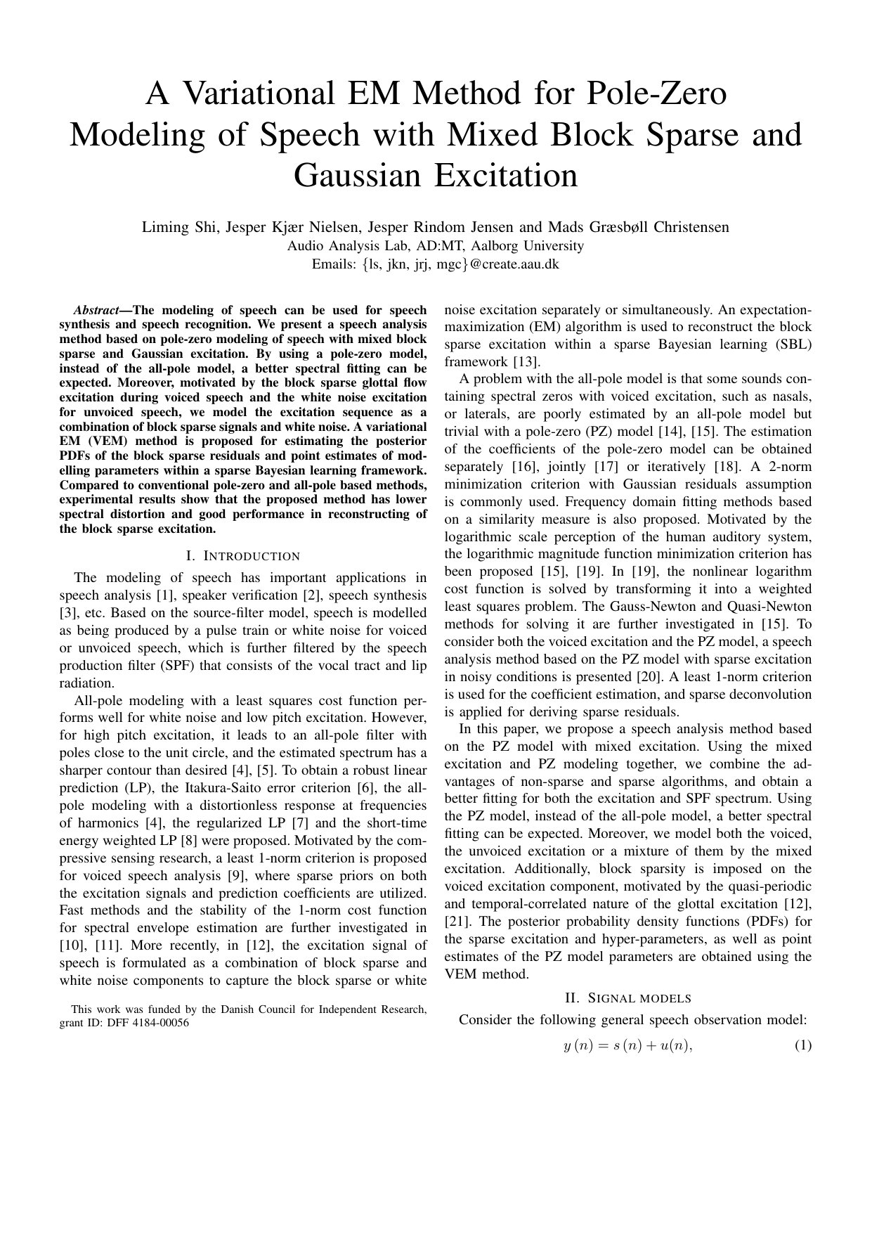 Figure 1
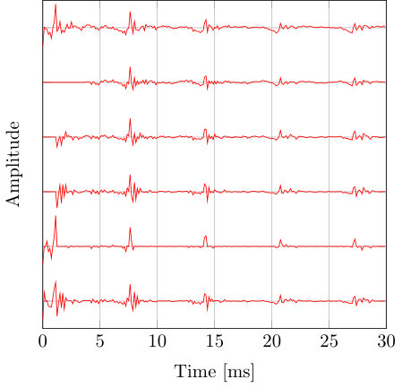 Figure 1
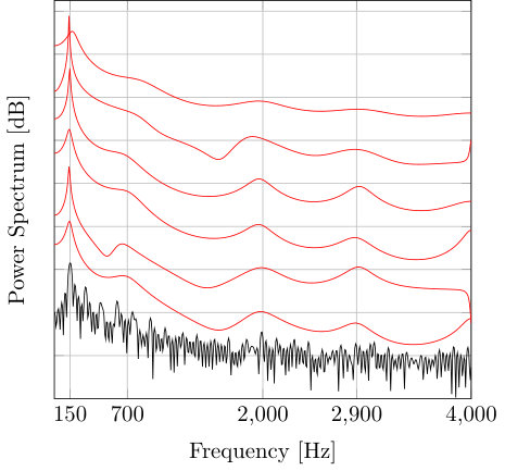 Figure 2
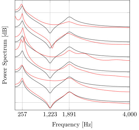 Figure 3
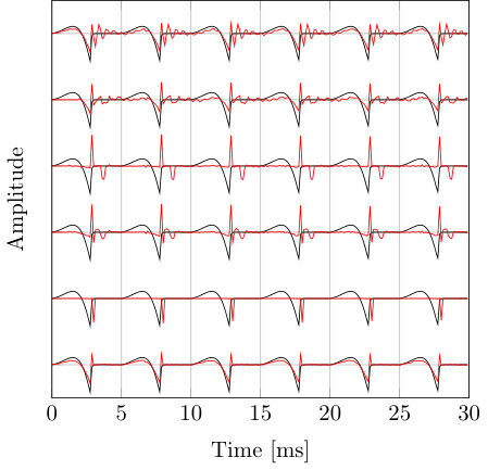 Figure 4
| F0 | 200 | 250 | 300 | 350 | 400 |
|---|---|---|---|---|---|
| 2-norm LP | 1.79 | 2.14 | 2.12 | 2.53 | 2.13 |
| TS-LS-PZ | 2.41 | 4.77 | 1.88 | 1.46 | 2.86 |
| 1-norm LP | 2.43 | 3.15 | 3.60 | 3.29 | 4.29 |
| EM-LP | 5.62 | 6.68 | 4.68 | 3.96 | 4.83 |
| VEM-PZ, D=1 | 4.50 | 7.14 | 2.29 | 1.54 | 2.31 |
| VEM-PZ, D=5 | 1.55 | 4.47 | 0.69 | 2.01 | 4.50 |
| VEM-PZ, D=7 | 2.08 | 4.07 | 2.18 | 1.41 | 1.29 |
| VEM-PZ, D=8 | 0.77 | 5.56 | 2.52 | 4.86 | 0.53 |
Peer Reviews
No public reviews on file for this paper yet. If you reviewed it on a platform where reviews are public (OpenReview, ICLR, NeurIPS, ICML), you can paste yours below so the community can read it here.
Videos
No videos yet. Explain this paper in a talk, walkthrough, or lecture? Add one.
Taxonomy
TopicsSpeech and Audio Processing · Speech Recognition and Synthesis · Blind Source Separation Techniques
A Variational EM Method for Pole-Zero
Modeling of Speech with Mixed Block Sparse and Gaussian Excitation
Liming Shi, Jesper Kjær Nielsen, Jesper Rindom Jensen and Mads Græsbøll Christensen This work was funded by the Danish Council for Independent Research, grant ID: DFF 4184-00056 Audio Analysis Lab, AD:MT, Aalborg University
Emails: {ls, jkn, jrj, mgc}@create.aau.dk
Abstract
The modeling of speech can be used for speech synthesis and speech recognition. We present a speech analysis method based on pole-zero modeling of speech with mixed block sparse and Gaussian excitation. By using a pole-zero model, instead of the all-pole model, a better spectral fitting can be expected. Moreover, motivated by the block sparse glottal flow excitation during voiced speech and the white noise excitation for unvoiced speech, we model the excitation sequence as a combination of block sparse signals and white noise. A variational EM (VEM) method is proposed for estimating the posterior PDFs of the block sparse residuals and point estimates of modelling parameters within a sparse Bayesian learning framework. Compared to conventional pole-zero and all-pole based methods, experimental results show that the proposed method has lower spectral distortion and good performance in reconstructing of the block sparse excitation.
I Introduction
The modeling of speech has important applications in speech analysis [1], speaker verification [2], speech synthesis[3], etc. Based on the source-filter model, speech is modelled as being produced by a pulse train or white noise for voiced or unvoiced speech, which is further filtered by the speech production filter (SPF) that consists of the vocal tract and lip radiation.
All-pole modeling with a least squares cost function performs well for white noise and low pitch excitation. However, for high pitch excitation, it leads to an all-pole filter with poles close to the unit circle, and the estimated spectrum has a sharper contour than desired [4, 5]. To obtain a robust linear prediction (LP), the Itakura-Saito error criterion [6], the all-pole modeling with a distortionless response at frequencies of harmonics [4], the regularized LP [7] and the short-time energy weighted LP [8] were proposed. Motivated by the compressive sensing research, a least 1-norm criterion is proposed for voiced speech analysis [9], where sparse priors on both the excitation signals and prediction coefficients are utilized. Fast methods and the stability of the 1-norm cost function for spectral envelope estimation are further investigated in [10, 11]. More recently, in [12], the excitation signal of speech is formulated as a combination of block sparse and white noise components to capture the block sparse or white noise excitation separately or simultaneously. An expectation-maximization (EM) algorithm is used to reconstruct the block sparse excitation within a sparse Bayesian learning (SBL) framework [13].
A problem with the all-pole model is that some sounds containing spectral zeros with voiced excitation, such as nasals, or laterals, are poorly estimated by an all-pole model but trivial with a pole-zero (PZ) model [14, 15]. The estimation of the coefficients of the pole-zero model can be obtained separately [16], jointly [17] or iteratively [18]. A 2-norm minimization criterion with Gaussian residuals assumption is commonly used. Frequency domain fitting methods based on a similarity measure is also proposed. Motivated by the logarithmic scale perception of the human auditory system, the logarithmic magnitude function minimization criterion has been proposed [19, 15]. In [19], the nonlinear logarithm cost function is solved by transforming it into a weighted least squares problem. The Gauss-Newton and Quasi-Newton methods for solving it are further investigated in [15]. To consider both the voiced excitation and the PZ model, a speech analysis method based on the PZ model with sparse excitation in noisy conditions is presented [20]. A least 1-norm criterion is used for the coefficient estimation, and sparse deconvolution is applied for deriving sparse residuals.
In this paper, we propose a speech analysis method based on the PZ model with mixed excitation. Using the mixed excitation and PZ modeling together, we combine the advantages of non-sparse and sparse algorithms, and obtain a better fitting for both the excitation and SPF spectrum. Using the PZ model, instead of the all-pole model, a better spectral fitting can be expected. Moreover, we model both the voiced, the unvoiced excitation or a mixture of them by the mixed excitation. Additionally, block sparsity is imposed on the voiced excitation component, motivated by the quasi-periodic and temporal-correlated nature of the glottal excitation [21, 12]. The posterior probability density functions (PDFs) for the sparse excitation and hyper-parameters, as well as point estimates of the PZ model parameters are obtained using the VEM method.
II Signal models
Consider the following general speech observation model:
[TABLE]
where is the observation signal and denotes the noise. We assume that the clean speech signal is produced by the PZ speech production model, i.e.,
[TABLE]
where and are the modeling coefficients of the PZ model with , is a sparse excitation corresponding to the voiced part and is the non-sparse Gaussian excitation component corresponding to the unvoiced part. Assuming and considering one frame of speech signals of samples, (1) and (2) can be written in matrix forms as
[TABLE]
where and are the lower triangular Toeplitz matrices with and as the first columns, respectively. The block sparse residuals are defined as , and , , and are defined similarly to . When , reduces to the identity matrix and (4) becomes the all-pole model. Combining (3) and (4), the noisy observation can be written as
[TABLE]
In [20], we assumed that only the sparse excitation was present (, but ). The sparse residuals and model parameters were estimated iteratively. The sparse residuals were obtained by solving
[TABLE]
where is a constant proportional to the variance of the noise. The model parameters was estimated using the norm of the residuals as the cost function (see [20] for details).
III Proposed Variational EM method
We now proceed to consider the noise-free scenario but with mixed excitation (, but ). We consider the pole-zero model parameters and to be deterministic but unknown. Utilizing the SBL [13] methodology, we first express the hierarchical form of the model as
[TABLE]
where is the number of blocks, , is the Kronecker product, is the block size, , denotes the multivariate normal PDF and is the Gamma PDF. The hyperparameter is the precision of the block, and when it is infinite, the block will be zero. Note that it is trivial to extend the proposed method to any . Moreover, when , each element in is inferred independently. Here, block sparsity model is used to take the quasi-periodic and temporal-correlated nature of the voiced excitation into account. The is used for capturing the white noise excitation from unvoiced speech frame or a mixture of phonations.
Our objective is to obtain the posterior densities of , and , and point estimates of the model parameters in and . First, we write the complete likelihood, i.e.,
[TABLE]
where we used when . Instead of finding the joint posterior density , which is intractable, we adopt the variational approximation [22]. Assume that is approximated by the density , which may be fully factorized as
[TABLE]
where the factors are found using an EM-like algorithm [22].
In the E-step of the VEM method, we fix the model parameters and , and re-formulate the posterior PDFs estimation problem as maximizing the variational lower bound
[TABLE]
where is the shorthand for , is defined as , and denotes the expectation of w.r.t. the random variable (i.e., ). Substituting (III) and (9) into (10), and following the derivation from [22], we obtain
[TABLE]
It is clearly seen that in (III) is a Gaussian PDF, i.e.,
[TABLE]
where and . We also define the auto-correlation matrix . The posterior PDF of in (III) is a Gamma probability density, i.e.,
[TABLE]
where , and denotes the element of . The expectation of the precision matrix is . Similar to , the posterior PDF of is
[TABLE]
where , . The expectation of can be expressed as .
In the M-step, we maximize the lower bound (10) w.r.t. the modeling parameters and , respectively. The optimization problems can be shown to be equivalent to , respectively. To obtain the estimate for , we first note that can be expressed as , where is a Toeplitz matrix of the form
[TABLE]
Using this expression and obtained in the E-step, the minimization problem w.r.t. can be re-formulated as
[TABLE]
As can be seen, (III) is the standard least squares problem and has the analytical solution as
[TABLE]
We can obtain the solution of , like , by setting the derivative of w.r.t. to zero, i.e.,
[TABLE]
where is an lower triangular Toeplitz matrix of the form
[TABLE]
From (III), we obtain the estimate of , i.e.,
[TABLE]
where is an symmetric matrix with the element given by . The can be obtained by simply replacing the stochastic variable in with the mean estimate (the element in ). The is an vector with the element given by . Note that the estimation of in (18) requires the knowledge of and vice versa (see (16)). This coupling is solved by replacing them with their estimates from previous iteration. The algorithm is initialized with , , and , and starts with the update of . We refer to the proposed variational expectation maximization pole-zero estimation algorithm as the VEM-PZ.
IV Results
In this section, we compare the performance of the proposed VEM-PZ, the two-stage least squares pole-zero (TS-LS-PZ) method [14], 2-norm linear prediction (2-norm LP) [1], 1-norm linear prediction (1-norm LP)[9] and expectation maximization based linear prediction (EM-LP) for mixed excitation [12] in both synthetic and real speech signals analysis scenarios.
IV-A Synthetic signal analysis
The reference list from the paper itself. Each links out to its DOI / PubMed record.
- 1[1] J. Makhoul, “Linear prediction: A tutorial review,” Proc. IEEE , vol. 63, no. 4, pp. 561–580, 1975.
- 2[2] J. Pohjalainen, C. Hanilci, T. Kinnunen, and P. Alku, “Mixture linear prediction in speaker verification under vocal effort mismatch,” IEEE Signal Process. Lett. , vol. 21, no. 12, pp. 1516–1520, dec 2014.
- 3[3] D. Erro, I. Sainz, E. Navas, and I. Hernaez, “Harmonics plus noise model based vocoder for statistical parametric speech synthesis,” IEEE J. Sel. Topics Signal Process. , vol. 8, no. 2, pp. 184–194, 2014.
- 4[4] M. N. Murthi and B. D. Rao, “All-pole modeling of speech based on the minimum variance distortionless response spectrum,” IEEE Trans. Speech Audio Process. , vol. 8, no. 3, pp. 221–239, 2000.
- 5[5] T. Drugman and Y. Stylianou, “Fast inter-harmonic reconstruction for spectral envelope estimation in high-pitched voices,” IEEE Signal Process. Lett. , vol. 21, no. 11, pp. 1418–1422, 2014.
- 6[6] A. El-Jaroudi and J. Makhoul, “Discrete all-pole modeling,” IEEE Trans. Signal Process. , vol. 39, no. 2, pp. 411–423, 1991.
- 7[7] L. A. Ekman, W. B. Kleijn, and M. N. Murthi, “Regularized linear prediction of speech,” vol. 16, no. 1, pp. 65–73, 2008.
- 8[8] P. Alku, J. Pohjalainen, M. Vainio, A. M. Laukkanen, and B. H. Story, “Formant frequency estimation of high-pitched vowels using weighted linear prediction.” J. Acoust. Soc. Am. , vol. 134, no. 2, pp. 1295–1313, Auguest 2013.