A practical fpt algorithm for Flow Decomposition and transcript assembly
Kyle Kloster, Philipp Kuinke, Michael P. O'Brien, Felix Reidl,, Fernando S\'anchez Villaamil, Blair D. Sullivan, and Andrew van der Poel

TL;DR
This paper introduces a practical fixed-parameter tractable algorithm for Flow Decomposition in DAGs, crucial for transcript assembly, and demonstrates its efficiency and exactness on RNA-sequence data.
Contribution
The paper presents the first practical linear FPT algorithm for Flow Decomposition, along with an implementation that outperforms heuristics in transcript assembly tasks.
Findings
The solver finds exact solutions efficiently on RNA-sequence data.
The algorithm's runtime is competitive with state-of-the-art heuristics.
Hardness results show no polynomial kernels and NP-hardness for related problems.
Abstract
The Flow Decomposition problem, which asks for the smallest set of weighted paths that "covers" a flow on a DAG, has recently been used as an important computational step in transcript assembly. We prove the problem is in FPT when parameterized by the number of paths by giving a practical linear fpt algorithm. Further, we implement and engineer a Flow Decomposition solver based on this algorithm, and evaluate its performance on RNA-sequence data. Crucially, our solver finds exact solutions while achieving runtimes competitive with a state-of-the-art heuristic. Finally, we contextualize our design choices with two hardness results related to preprocessing and weight recovery. Specifically, -Flow Decomposition does not admit polynomial kernels under standard complexity assumptions, and the related problem of assigning (known) weights to a given set of paths is NP-hard.
Click any figure to enlarge with its caption.
 Figure 1
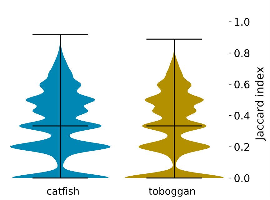 Figure 2
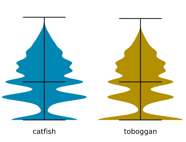 Figure 3
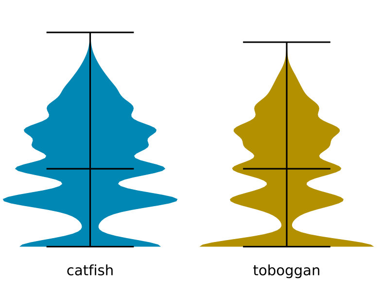 Figure 4
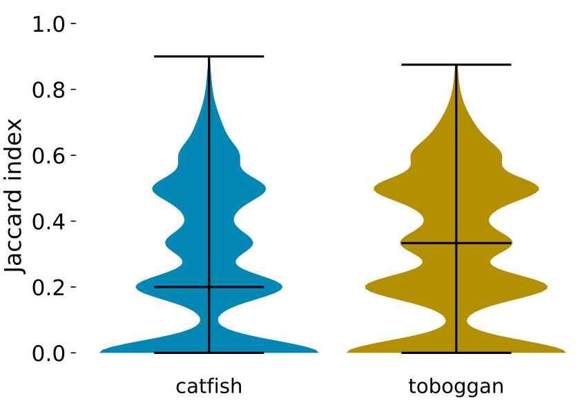 Figure 5
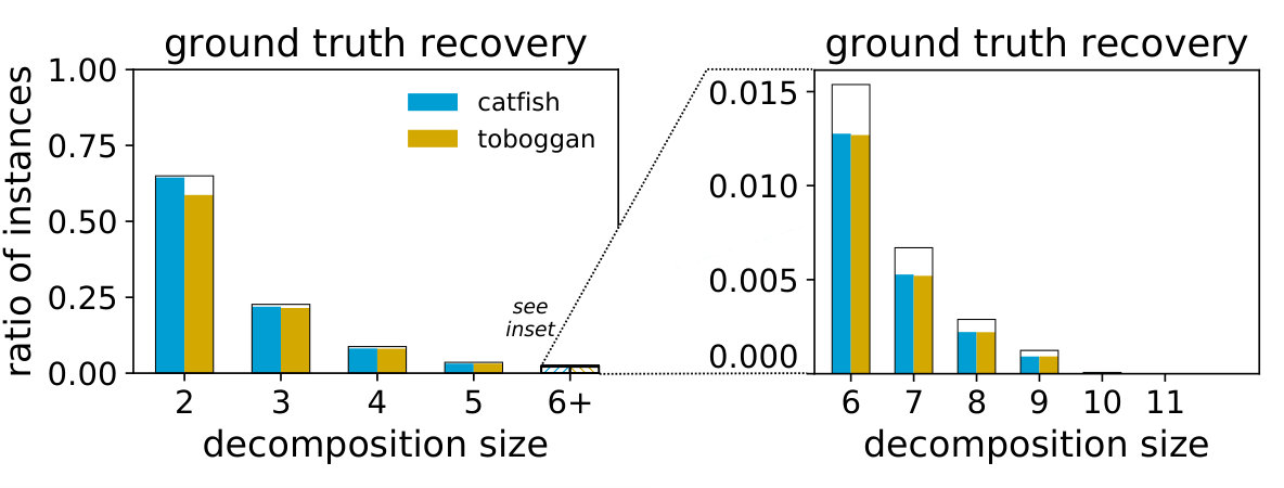 Figure 6
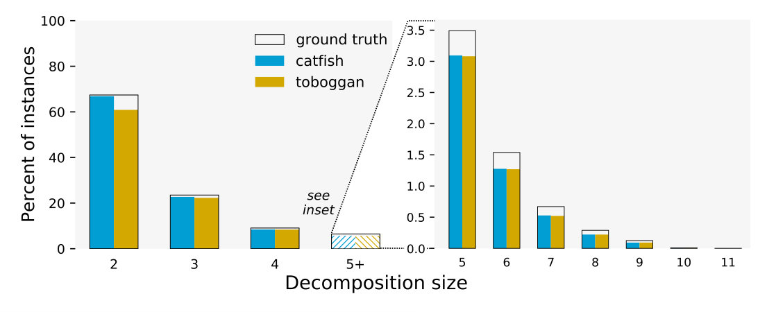 Figure 7
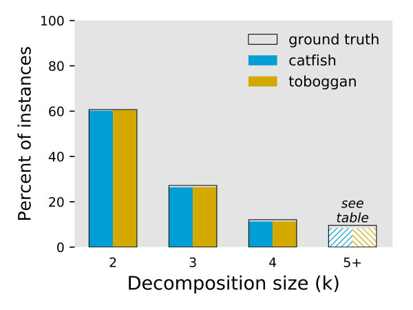 Figure 8
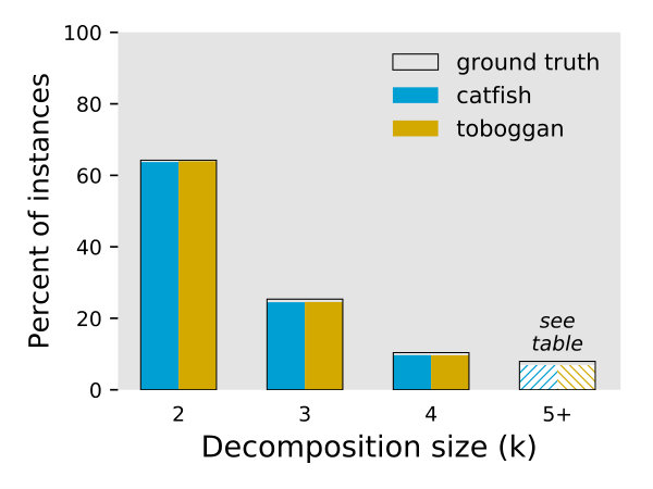 Figure 9
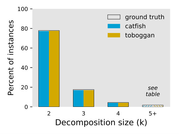 Figure 10
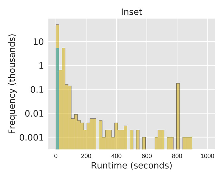 Figure 11
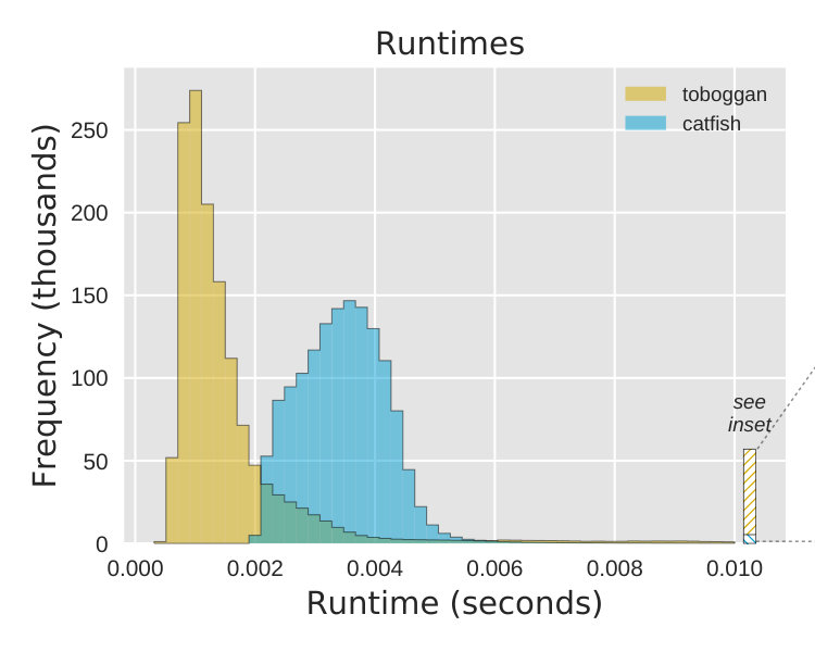 Figure 12
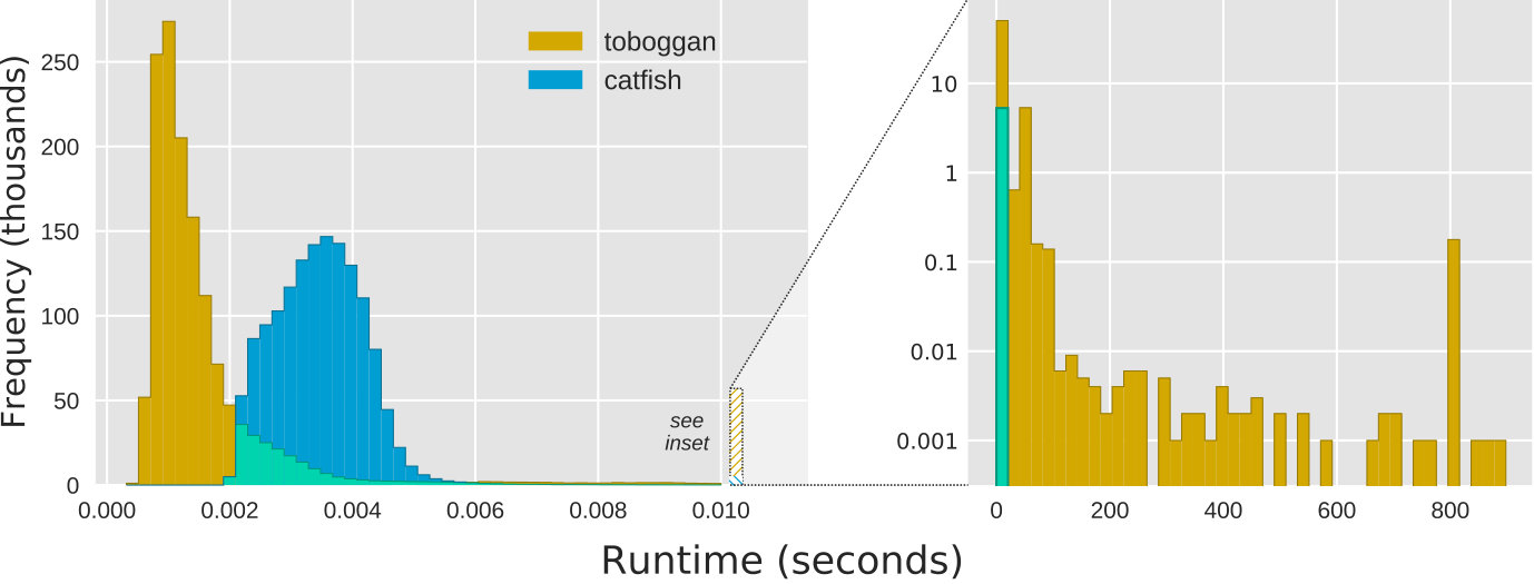 Figure 13
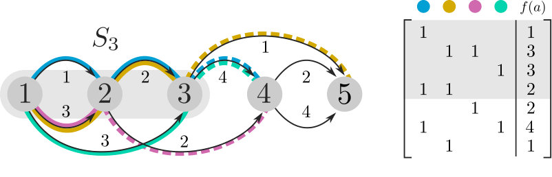 Figure 14
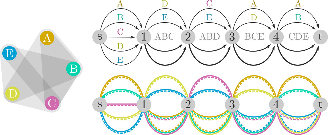 Figure 15
| dataset | instances | non-trivial | nodes | deg | optimal | non-optimal | |
|---|---|---|---|---|---|---|---|
| zebrafish | 1,549,373 | 445,880 | 18.49 | 2.27 | 2.32 | 99.91% | 0.053% |
| mouse | 1,316,058 | 473,185 | 18.67 | 2.37 | 2.75 | 99.40% | 0.074% |
| human | 1,169,083 | 529,523 | 18.79 | 2.41 | 2.83 | 99.49% | 0.043% |
| human-salmon | 13,300,893 | 7,153,472 | 20.54 | 2.55 | 3.74 | 94.39% | 0.035% |
| all | 17,335,407 | 8,602,060 | 20.22 | 2.52 | 3.55 | 95.27% | 0.039% |
Peer Reviews
No public reviews on file for this paper yet. If you reviewed it on a platform where reviews are public (OpenReview, ICLR, NeurIPS, ICML), you can paste yours below so the community can read it here.
Videos
No videos yet. Explain this paper in a talk, walkthrough, or lecture? Add one.
\reserveinserts
28
\CopyrightKyle Kloster, Philipp Kuinke, Michael O’Brien, Felix Reidl, Fernando Sánchez Villaamil,
Under Logo Blair D. Sullivan, Andrew van der Poel
A practical fpt algorithm for Flow Decomposition and transcript assembly
Kyle Kloster
North Carolina State University, USA
(kakloste|mpobrie3|blair_sullivan|ajvande4)@ncsu.edu, [email protected]
Philipp Kuinke
RWTH Aachen University, Germany
(kuinke|fernando.sanchez)@cs.rwth-aachen.de
Michael P. O’Brien
North Carolina State University, USA
(kakloste|mpobrie3|blair_sullivan|ajvande4)@ncsu.edu, [email protected]
Felix Reidl
North Carolina State University, USA
(kakloste|mpobrie3|blair_sullivan|ajvande4)@ncsu.edu, [email protected]
Fernando Sánchez Villaamil
RWTH Aachen University, Germany
(kuinke|fernando.sanchez)@cs.rwth-aachen.de
Blair D. Sullivan
North Carolina State University, USA
(kakloste|mpobrie3|blair_sullivan|ajvande4)@ncsu.edu, [email protected]
Andrew van der Poel
North Carolina State University, USA
(kakloste|mpobrie3|blair_sullivan|ajvande4)@ncsu.edu, [email protected]
Abstract.
The Flow Decomposition problem, which asks for the smallest set of weighted paths that “covers” a flow on a DAG, has recently been used as an important computational step in transcript assembly. We prove the problem is in when parameterized by the number of paths by giving a practical linear fpt algorithm. Further, we implement and engineer a Flow Decomposition solver based on this algorithm, and evaluate its performance on RNA-sequence data. Crucially, our solver finds exact solutions while achieving runtimes competitive with a state-of-the-art heuristic. Finally, we contextualize our design choices with two hardness results related to preprocessing and weight recovery. Specifically, -Flow Decomposition does not admit polynomial kernels under standard complexity assumptions, and the related problem of assigning (known) weights to a given set of paths is -hard.
Key words and phrases:
1. Introduction
We study the problem Flow Decomposition [6, 10, 16, 19] under the paradigm of parameterized complexity [4]. Motivated by the principles of algorithm engineering, we design and implement an fpt algorithm that not only solves the problem exactly but also has a run- time that is competitive with heuristics [16, 19]. Furthermore, we characterize several key aspects of the problem’s complexity. Decomposing flows is the central algorithmic problem in a recent method for analyzing high-throughput transcriptomic sequencing data, and we benchmark our implementation on data from this use case [16].
Flow Decomposition asks for the minimum number of weighted paths necessary to exactly cover a flow on a directed acyclic graph with a unique source and sink (an -–DAG). More precisely, we say a set of -–paths and corresponding weights are a flow decomposition of an -–DAG with flow if
[TABLE]
for every arc in , where is the indicator function whose output is 1 if , and [math] otherwise. Specifically, in this paper, we are concerned with -Flow Decomposition, which uses the natural parameter of the number of paths.
Problem 1.1**.**
*-Flow Decomposition (-FD) \Input& () with an -–DAG, a flow on , and a positive integer.
\Prob Is there an integral flow decomposition of using at most paths?*
Shao and Kingsford recently used flow decompositions to assemble unknown transcripts from observed subsequences of RNA called exons [16]. In this context, the input graph is a splice graph, which is constructed in one of two ways: either by contracting induced paths in a de Bruijn graph (de novo assembly) or by connecting exons inferred from an alignment process that co-occur in reads (reference-based). In both constructions, every vertex in the graph corresponds to a (partial) exon being transcribed and every arc indicates that two exons appear in sequence in one of the reads; the arcs are weighted based on abundance (frequency) in the data. If we affix a dummy source and a dummy sink to the vertices of in- and out-degree zero, respectively, the resulting labeling forms a flow111This assumes an idealized scenario with constant read coverage, but methods exist to rectify noisy data [18]. from to . As such, a transcript corresponds to a weighted -–path and we aim to recover the collection of transcripts by decomposing the flow into a minimal number of paths in the above sense.
A precursory investigation of the data used by Shao and Kingsford [16] to evaluate the performance of Flow Decomposition heuristics in RNA transcript assembly left us with three guiding observations:
- (1)
97% of instances admit decompositions into fewer than 8 paths. Our algorithm should thus exploit the small natural parameter. 2. (2)
The data set contains over 17 million mostly small instances. Our implementation should therefore be able to handle a large throughput. 3. (3)
The flow decompositions computed by our implementation should reliably recover the domain-specific solution i.e. the true transcripts.
The first point corroborates the parameterized approach. Using dynamic programming over a suitable graph decomposition, a common algorithm design technique from parameterized complexity, we show the problem can be solved in linear-fpt time (Section 3):
Theorem 1.2**.**
There is an algorithm for solving -Flow Decomposition, where is the logarithm of the largest flow value.
To address the second point, we implement a Flow Decomposition solver, Toboggan [7], based on this algorithm and compare it with the state-of-the-art heuristic Catfish (Section 5). Our results show that Toboggan’s running time is comparable to Catfish and thus suitable for high-throughput applications. With respect to the third point, using Flow Decomposition for assembly implicitly assumes that the true transcripts correspond to paths in a minimum-size flow decomposition. Prior work focuses on heuristics which cannot be used to evaluate the validity of this assumption. With Toboggan, we validate that minimum-size flow decompositions accurately recover transcripts in most instances (Section 5.3).
Toboggan incorporates several heuristic improvements (discussed in Section 4) to keep the running time and memory consumption of the core dynamic programming routine as small as possible. In particular, the simple preprocessing we employ is highly successful in solving many instances directly. A provable guarantee for this preprocessing in the form of a small kernel, however, is unlikely: we show that unless is contained in {\mathchoice{\hbox{\mathsf{coNP}}}{\hbox{\mathsf{coNP}}}{\mathsf{coNP}}{\mathsf{coNP}}}/\emph{poly}, -FD does not admit a polynomial kernel (Section 6). Further, our experimental evaluation hints at the following conjecture: for a given decomposition of an -–DAG into a minimum number of paths, there is a unique assignment of weights to those paths to achieve a flow-decomposition. If the conjecture holds, it implies a tighter bound on the running time of the algorithm in Theorem 1.2. Despite this, we prove the more general ‘weight recovery’ problem is -hard given a decomposition into an arbitrary number of paths (Section 7).
2. Preliminaries
Related work.
Flow Decomposition is known to be -complete, even when all flow values are in , and does not admit a PTAS [6, 19]. The best known approximation algorithm for the problem is based on parity-balancing path flows [10], and guarantees an approximation ratio of with a running-time of , where is the length of the longest -–path, and is the logarithm of the maximum flow value. The variant in which the decomposition approximates the original flow values to minimize a specified penalty function was studied in [17], and the authors give an fpt algorithm and FPTAS parameterized by , the largest --cut, and the maximum flow value.
Due to its practical use for sequencing data, much of the prior work on Flow Decomposition has focused on fast heuristics, including two greedy algorithms which iteratively add the remaining path which is shortest (greedy-length) or of maximum possible weight (greedy-width) [19]. Both heuristics produce solutions with at most paths and have variants [6] which decompose all but an -fraction of the flow using at most times the minimum number of paths, for any . Historically, greedy-width has provided the best performance [6, 10, 19], but the recent heuristic Catfish [16] showed significant improvements over greedy-width in accuracy and runtime.
Notation.
Given a directed acylic graph (DAG), , we say is an -–DAG if has a single source, , and a single sink, . We denote by the set of out-arcs of a node , and by the in-arcs. For a set of nodes, , we define . If is a flow on , we write for the flow value on an arc and for the total flow (the sum of flow values on the arcs in ).
Terminology.
Given a DAG, a topological ordering on the nodes is a labeling such that every arc is directed from a node with a smaller label to one with a larger label. We label the nodes of an -–DAG as corresponding to an arbitrary, fixed topological ordering of ; this implies that and . We further define the sets based on the ordering. We refer to the -–cuts as topological ordering cuts (top-cuts). Our algorithm for computing a flow decomposition will ultimately depend on tracking how the paths cross top-cuts, a notion we refer to as a routing.
Definition 2.1** (Routings and extensions).**
A surjective function is a routing out of . A routing is an extension of if for each , implies if , and for some if .
In other words, an extension of a routing takes all the integers that map to in-arcs of and maps them instead to the out-arcs of (because it is surjective) while leaving the rest of the mapping unchanged. It will be important in our analysis to differentiate arcs that occur in multiple paths from arcs that appear on only a single path: we say paths and coincide on arc if and . An arc is saturated by a path if is the only path for which .
Parameterized complexity.
A parameterized decision problem is fixed parameter tractable if there exists an algorithm that decides it in time for some computable function and a constant . When , we call such an algorithm linear fpt. A polynomial kernel is an algorithm that transforms, in polynomial time, an instance of into an equivalent instance with , meaning that if and only if . Some more advanced machinery pertaining to kernelization lower bounds will be defined in Section 6.
3. A linear fpt algorithm for -FD
We solve -FD via dynamic programming over the topological ordering: we enumerate all ways of routing -–paths over each top-cut . Each such routing determines a set of constraints for the path weights, which we encode in linear systems. For example, if paths and are routed over an arc , we add the constraint to our system.
Concretely, we keep a table for whose entries are sets of pairs , where is a routing of the paths out of and is a system of linear equations that encodes the known path weight constraints. In particular, for every arc , we write for the set of -–paths that are routed over . Each system of linear equations, , is of the form , where is a binary matrix with columns, is the solution weight vector, and is a vector containing values of . Each row of corresponds to an arc and encodes the constraint that the weights of paths routed over sum up to . The th entry of row is 1 if and only if path was routed over , and then equals the th entry of . Figure 1 illustrates an example of an entry .
We now describe how the dynamic programming tables are constructed. For ease of description, we augment to have two additional dummy arcs and , where is an in-arc of and is an out-arc of and . We begin with table that has a single entry. The routing of this entry routes all paths over and the linear system has a single row that constrains all path weights to sum to the total flow value.
For , we construct the table from . Conceptually, we “visit” node and “push” all paths routed over its in-arcs to be routed over its out-arcs. Formally, we require the routing out of to be an extension (Definition 2.1) of a routing out of . For each entry we compute an entry of for each extension of . For a given , we create by adding a row to for each arc , encoding the constraint
[TABLE]
At the conclusion of the dynamic programming, all entries of the final table will have the same routing, since has one (dummy) out-arc . This table allows us to decide whether there is a solution; is a yes-instance of -FD if and only if some has a solution whose entries are positive integers. Pseudocode for our algorithm can be found in Algorithm 1 in Appendix A.
Lemma 3.1**.**
An integer vector is a solution to if and only if there is a set of -–paths such that is a flow decomposition of .
Proof 3.2**.**
We first prove the forward direction. If we keep backpointers in our DP tables i.e. pointers from entry to the entry in the previous table for which was the extension of , we can obtain a sequence of routings that correspond to backwards traversal of the backpointers. Let . By Definition 2.1, removing the duplicate elements that appear in consecutive order from yields a series of arcs that form an -–path . Because each routing requires every arc to have a path routed over it, the system contains constraints corresponding to each arc. Thus an integer solution to corresponds to a weighting of such is a flow decomposition.
In the reverse direction, we first observe that the incidence of paths in on a top-cut corresponds to a routing out of . Let be the corresponding routing out of . For each node , the paths routed over must immediately be routed over an arc in , meaning is an extension of . Because is a flow decomposition, the paths routed over each arc will have weights summing to the flow value on that arc. Thus, any constraint in a linear system associated with the routings will have as a solution.
To analyze the running time we now derive bounds on the dynamic programming table sizes. First, we bound the number of possible routings in Lemma 3.3, then we give an upper bound on the number of linear systems in Lemma 3.5.
Lemma 3.3**.**
There are at most routings of paths over any top-cut.
Proof 3.4**.**
A routing of paths over a top-cut can be thought of as a partition of the paths into many non-empty sets along with a mapping of these sets to the arcs of . We can assume that , since a routing of paths requires every top-cut to have at most arcs. The number of ways to partition objects into non-empty sets is , the Stirling number of the second kind, and there are ways to assign each of these partitions to a specific arc. Thus, the number of routings is . To proceed, we use the upper bound due to Rennie and Dobson [12]. We also make use of the tighter version of Stirling’s approximation due to Robbins [13], which states that
[TABLE]
Hence, we have the upper bound
[TABLE]
Letting for , the above expression becomes
[TABLE]
where the constant can be derived numerically by maximizing on the interval .
Lemma 3.5**.**
Each table has at most distinct linear systems.
Proof 3.6**.**
Without loss of generality, we can ensure each linear system has at most rows by removing linearly dependent rows. We note that because there are only subsets of weights, if maps the arcs to more than unique flow values, there cannot be a flow decomposition of size . Since the elements of can thus take on at most many values, and contains binary rows of length , it follows that there are at most rows for . Accordingly, we can bound the number of possible linear systems by . By imposing an order on the rows we can remove a factor of . Because , we can apply the bound which holds [8] for ; thus, the number of linear systems is at most .
Now that we have bounded the size of the dynamic programming tables, we analyze the complexity of solving the linear systems in the final table . It has been shown that treating linear systems as integer linear programs (ILPs) produces integer solutions in fpt-time.
Proposition 3.7** ([9]).**
Finding an integer solution to a given system takes time at most , where is the encoding size of the linear system.
These results give the following upper bound on the runtime of our algorithm, proving Theorem 1.2.
Theorem 3.8**.**
Algorithm 1 solves -FD in time where is the logarithm of the largest flow value of the input.
Proof 3.9**.**
The correctness of the algorithm was already proven in Lemma 3.1, so all that remains is to bound the running time. By Lemmas 3.3 and 3.5, the total number of elements in DP table is bounded by
[TABLE]
Reducing the linear systems and checking for consistency is polynomial in the size of the matrix (which is ). Finally, we need to find a feasible solution among all the linear systems left after the last DP step. We apply Proposition 3.7 to these systems, whose encoding size is bounded by . We arrive at the desired running time of
[TABLE]
where we use the well-known bound .
4. Implementation
To establish that our exact algorithm for -FD is a viable alternative to the heuristics currently in use by the computational biology community, we implemented Algorithm 1 as the core of a Flow Decomposition solver Toboggan [7]. The solver iterates over values of in increasing order until reaching a yes-instance of -FD. Toboggan also implements backtracking to recover the -–paths. Making Toboggan’s runtime competitive with existing implementations of state-of-the-art heuristics required non-trivial algorithm engineering. Our improvements broadly fall into three categories: preprocessing, pruning, and low-memory strategies for exploring the search space. The remainder of this section describes the most noteworthy techniques implemented in Toboggan that are not captured by Algorithm 1.
4.1. Preprocessing
Toboggan implements two key preprocessing routines. The first generates an equivalent instance on a simplified graph using a series of arc contractions. The second calculates lower bounds on feasible values of to reduce the number of calls to the -FD solver.
Graph reduction.
We first reduce the graph by contracting all arcs into/out of nodes of in-/out-degree 1. We prove in Lemma 4.1 that given a flow decomposition of the contracted graph, we can efficiently recover a decomposition of the same size for the original graph.
Lemma 4.1**.**
Let be an arc for which or and the graph created by contracting . Then has a flow decomposition of size iff has a flow decomposition of size . Moreover, we can construct from in polynomial time.
Proof 4.2**.**
We first note that if is the graph formed by reversing the directions of the arcs in , any solution to can be transformed into a solution to by reversing the order of the paths and maintaining the same weights. Since this reversal is involutive, the correspondence between solutions to and is bijective, so it suffices to consider the case .
Given with a node that has , let be the graph with arc contracted. Given a flow decomposition of , we construct a corresponding decomposition for as follows. Every path containing must have as the vertex succeeding . Removing from each such will create a valid path in , since becomes part of in . Moreover, the incidence of paths on each other arc remains unchanged, so the solution covers the flows in .
In the reverse direction, consider a labeling of the arcs of such that we can distinguish among the in-arcs of those which exist in from those that result from contracting . Let be the set of latter arcs. We construct from as follows. For each path , if is routed over we modify to include the arcs and , rather than the arc , and add the modified path to . If no such arc lies in , we simply add to .
As in the forward direction, it is clear that any arcs in without as an endpoint have their flow values covered by , and that every path in is an -–path in . Since is derived from an arc , if are the paths routed over and is the set of paths corresponding to in , then exactly covers . Since every path in routed through subsequently is routed over and the flow values on the in-arcs of sum to , is also covered by . Thus is a valid solution to .
Lower bounds on .
To reduce the number of values of that Toboggan considers before reaching a yes-instance, we compute a lower bound on the optimal value of . One immediate lower bound is the size of the largest top-cut; we implement this in conjunction with the additional bound established in Lemma 4.3. Intuitively, if two top-cuts share few common flow values, many of the arcs must have multiple paths routed over them.
Lemma 4.3**.**
Given a flow , let and be any two top-cuts with . Letting be the multiset of flow values occurring in , set and . If has a flow decomposition of size , then
[TABLE]
and this lower bound is tighter than the cutset size iff .
Proof 4.4**.**
Suppose paths cross cutsets and . For every flow value in , it is possible a single path saturates the arc with that flow value in both cuts. Consider the remaining paths. To maximize the number of distinct flow values these paths produce, let each path saturate an arc in , yielding values in , and then route those paths in pairs across distinct arcs in . This produces at most new flow values in . This yields , and substituting for proves Inequality (1).
To prove the relationship between this lower bound and there are two cases. If , then by substituting we can upper bound . If instead , substituting yields .
4.2. Search Space Strategies
To reduce the memory required by dynamic programming, our implementation diverges from the pseudocode of Algorithm 1 in two ways. Specifically, we solve a restricted weight variant of -FD and use a separate phase to recover the -–paths.
Weight restriction.
Rather than making one pass through the dynamic programming that infers the solution weights from the linear systems, we employ a multi-pass strategy. Each pass restricts the potential weight vector by fixing a subset of its entries to weights chosen from flow values in the input instance while leaving the remaining values as variables to be determined by the DP routine. Since we observe that most instances in the data set (see Section 5.1) admit decompositions whose paths saturate at least one arc, we begin by enumerating potential weight-vectors whose values are all taken from flow values. If the DP routine finds no solution for any of these vectors, we enumerate vectors in which exactly one value is undetermined and all other entries are again taken from flow values, \etcIf all these attempts should fail, the final pass in our strategy will leave all weights to be determined by the DP and hence is guaranteed to find a solution, should one exist. For most instances, however, a solution vector is quickly guessed, vastly reducing the number of candidate linear systems in the DP and thus saving both time and memory.
Path recovery.
Computing the path weights requires storing only the current and previous dynamic programming tables in memory. In contrast, recovering the paths requires storing all dynamic programming tables. For this reason, we first determine the weights and then recover the paths by running the dynamic programming again with weights restricted to . This is equivalent to solving the -Flow Routing problem in Section 6.
4.3. Pruning
Within the dynamic programming we employ a number of heuristics that help recognize algorithmic states that cannot lead to a solution.
Weight bounds.
We augment the weight constraints imposed by the linear systems with a set of routing-independent constraints. These take the form of upper and lower bounds ( and , respectively) on the th smallest weight .
First, we compute by noting that for any top-cut and any arc , only paths can be routed over , i.e. . Then, we compute by finding the largest weight of any -–path. This can be done via a simple dynamic programming algorithm: for any node , an -–path with weight requires a path of equal weight to an in-neighbor such that .
To compute the bounds on the other weights, , we let be the smallest flow value and be the smallest222If no such flow value exists, set . flow value greater than . In other words, if , then must be part of a path of weight at least . Finally, we use these upper bounds to derive the s. If the weights greater than sum to , then by the pigeonhole principle , where is the total flow. Thus, .
For simplicity of implementation, we force the values of our weight vector to appear in non-decreasing order. In each dynamic programming table, for each linear system we run a linear program to see if there are any (rational) weights within the bounds that satisfy . If not, we remove the entry of the dynamic programming table containing . We also use these bounds before dynamic programming to catch partially determined weight vectors that will not be able to yield a solution. For example, the predetermined vector333A indicates an undetermined value. is incompatible with a lower bound on the third entry greater than 5.
Storing linear systems.
Within the dynamic programming we store linear systems in row-reduced echelon form (RREF). When a new row is introduced to the system, we perform Gaussian elimination to convert the new row to RREF, checking for linear dependence and inconsistency in time. The iterative row reduction also has the advantage of revealing determined path weights even if the system is not fully determined, and thus we can check whether any such values are not positive integers. Furthermore, once the system is full rank, no additional computation needs to be done to recover the weights.
5. Experimental Results
In this section we empirically evaluate the efficiency and solution quality of Toboggan by comparing with the current state-of-the-art, Catfish, on a corpus of simulated RNA sequencing data. Additionally, we use Toboggan to theoretically validate the -FD problem as a model for the transcript assembly task.
5.1. Experimental setup
Our experiments were run on a corpus of data used in previous experiments by Shao and Kingsford [15, 16]. The full data set contains over 17 million instances, each generated by simulating RNA-seq reads from a transcriptome and building the -–DAG and flow using the procedure described in Section 1. Two software packages were used to simulate reads: Flux Simulator [5], which used transcriptomes from humans, mice, and zebrafish, and Salmon [11], which only used human transcriptomes. We will refer to these four subsets as human, mouse, zebrafish, and human-salmon, respectively. The simulated reads allow us to know the true transcripts and thus the corresponding flow decomposition a priori; we will refer to this particular decomposition as the “ground truth”.
In our three experimental analyses (model validation, algorithm timing, and solution-quality) we report results on just the three smaller datasets (human, mouse, zebrafish). We terminated Toboggan on any run whose weight computation took longer than 800 seconds on zebrafish, and 50s on human and mouse 444Under these constraints, Toboggan timed out on of the 4M instances in these smaller data sets.. After performing more exhaustive computations on these smaller data sets, we then used the larger human-salmon data set (13.3M) to add one more data point for the model validation experiment. Because of the size of human-salmon, we terminated Toboggan after only 1 second. This smaller time limit resulted in Toboggan timing out on a significantly larger portion of human-salmon than the other three ( on human-salmon compared to on the other data sets), which would bias the results on human-salmon toward its simpler instances. Because of this, we omit the human-salmon results from the timing and solution-quality experiments.
For a small number of the 17M instances, the ground truth decomposition contains at least one path that appeared multiple times, corresponding to a subsequence repeated in different locations of the transcriptome. The data provides no means for mathematically or biologically distinguishing these; thus, we aggregated the duplicated paths into a single path, summing their weights. Additionally, we removed “trivial” instances in which the graph consisted of a single -–path; on such graphs Toboggan terminates during preprocessing without executing the -FD algorithm described in this paper. We remark that this is a departure from the experimental setup of Catfish, which included such graphs, explaining some slight differences in our statistics. About of the 17M graphs in the corpus are trivial in this manner. The number of non-trivial graphs for each species is summarized in Table 1. All experiments were run on a dedicated system with an Intel i7-3770 (3.40GHz, 8 cores), an 8192 KB cache, and 32 GB of RAM.
5.2. Benchmarking
We start by analyzing the efficiency of Toboggan and Catfish, noting that this compares a Python implementation [7] with C++ code [15]. Their runtimes on the 1.4M non-trivial instances in the smaller data sets are shown side-by-side in Figure 2. We observe that the two implementations are both quite fast on the vast majority of instances: their median runtimes are milliseconds (ms) (Toboggan) and ms (Catfish). However, the implementations have different runtime distributions—whereas Catfish is consistent, terminating between 2.3–4.6ms on of instances and never running longer than 1.3 seconds, Toboggan trades off faster termination, e.g. less than ms on of instances, with a higher variance and a small chance of a much longer runtime, e.g. over seconds on of instances.
5.3. Model Validation
Previous papers that use flow decompositions to recover RNA sequences [16, 18] implicitly assume that the true RNA sequences correspond to a minimum size flow decomposition, as opposed to one with an arbitrary number of paths. Because Toboggan provably finds the minimum size of a flow decomposition, our implementation enables us to investigate exactly how often this assumption holds in practice.
Table 1 gives the percentage of all non-trivial instances whose ground truth decompositions are in fact minimum decompositions, as well as the percentage of ground truth decompositions we proved have non-optimal size. We conclude from this table that the Flow Decomposition problem is in fact a useful model for transcript assembly, which underscores the need for efficient algorithms to compute minimum decompositions.
5.4. Ground Truth Recovery
Though the ground truth flow decompositions are almost always of minimum size, it is biologically desirable to find a particular minimum size decomposition rather than an arbitrary one. In this section we investigate how often the decompositions output by Toboggan and Catfish are identical to the ground truth decomposition, restricting our attention to non-trivial instances in which the ground truth decomposition is of minimum size. Additionally, for those instances where each algorithm does not exactly recover the ground truth, we analyze the similarity of the (imperfect) path set to the ground truth, using the Jaccard index.
The table in Figure 3 summarizes the performance of the Toboggan and Catfish implementations in exactly computing the ground truth decompositions. Their behavior was quite similar, with slight differences at each decomposition size, and a advantage for Toboggan overall.
For instances where an algorithm’s output is not identical to the ground truth, an output can still recover some useful information if it is highly similar to the ground truth decomposition. With this in mind, we evaluate how similar each algorithm’s output is to the ground truth when they do not exactly match555There are 43,817 such instances for Catfish and 41,783 for Toboggan.. The plot in Figure 3 shows the distribution of the Jaccard index of each algorithm’s output compared to the ground truth paths.
6. Kernelization lower bounds
As described in Section 4.1, our implementation employs a graph reduction algorithm that rapidly identifies any trivial graph and immediately solves Flow Decomposition. Out of the 17M total instances, this preprocessing solves all of the roughly 8.7M trivial instances. On non-trivial instances, Toboggan then tries to identify the correct number of paths in an optimal solution. The naïve lower bound from the largest edge cut is equal to the correct value of in of the 8.6M non-trivial instances; incorporating the bound from Lemma 4.3 brings this up to .
In the framework of parameterized complexity, it is therefore natural to ask whether -FD admits a polynomial kernel. Below we answer the question in the negative, despite the real-world success of our preprocessing. Our proof strategy requires hardness reductions involving the following restricted variants of Flow Decomposition.
Problem 6.1**.**
--Flow Decomposition* (-FD) \Input& An -–DAG, with an integral flow , an integer , and a set .
\Prob Does have a flow decomposition into paths whose weights are all members of ?*
Problem 6.2**.**
--Flow Routing* (-FR) \Input& An -–DAG, , integral flow , and integers taken from .
\Prob Is there a flow decomposition of into paths with respective weights ?*
Lemma 6.3**.**
--Flow Routing* is -complete.*
Proof 6.4**.**
Consider an instance of -FD, which is - complete [6]. Note that every -–path in a potential solution to such an instance can only take weights in . This enables us to Turing-reduce to at most instances of -FR: we simply guess how many of the -–paths use each of the three possible values. It follows that -FR is -complete.
In order to show that -FD does not admit polynomial kernels, we will provide a cross-composition from -FR. We first need the following technical definition to set up the necessary machinery:
Definition 6.5** (Polynomial equivalence relation [2]).**
An equivalence relation over is called a polynomial equivalence relation if the following hold:
- (1)
there exists an algorithm that decides for whether and are equivalent under in time polynomial in , and 2. (2)
for any finite set the index is bounded by a polynomial in .
The benefit of a polynomial equivalence relation is that we can focus on collection of instances which share certain characteristics, as long as these characteristics do not distinguish too many instances. A simple example is that we can ask for input instances in which all graphs have the same number of vertices and the values are the same.
Definition 6.6** (AND-cross-composition [2]).**
Let be a language, a polynomial equivalence relation over , and let be a parameterized problem. An AND-cross composition of into (under ) is an algorithm that, given instances of belonging to the same equivalence class of , takes time polynomial in and outputs an instance such that
- a)
the parameter is polynomially bounded in , and 2. b)
we have that if and only if all instances .
We will now use the following theorem (abridged to our needs here) and the subsequent AND-cross-composition to prove that -FD does not admit small kernels.
Proposition 6.7** (Bodlaender, Jansen, Kratsch [2]).**
If an -hard language AND-cross-composes into a parameterized problem , then does not admit a polynomial kernelization unless {\mathchoice{\hbox{\mathsf{NP}}}{\hbox{\mathsf{NP}}}{\mathsf{NP}}{\mathsf{NP}}}\subseteq{\mathchoice{\hbox{\mathsf{coNP}}}{\hbox{\mathsf{coNP}}}{\mathsf{coNP}}{\mathsf{coNP}}}/\emph{poly} and the polynomial hierarchy collapses.
Theorem 6.8**.**
-Flow Decomposition* does not admit a polynomial kernel unless {\mathchoice{\hbox{\mathsf{NP}}}{\hbox{\mathsf{NP}}}{\mathsf{NP}}{\mathsf{NP}}}\subseteq{\mathchoice{\hbox{\mathsf{coNP}}}{\hbox{\mathsf{coNP}}}{\mathsf{coNP}}{\mathsf{coNP}}}/\emph{poly} and the polynomial hierarchy collapses.*
Proof 6.9**.**
Let be the equivalence relation on instances of -FR where if and only if . Since each entry of is in , has at most equivalence classes, and is a polynomial equivalence relation.
Let be instances of -FR all contained in the same equivalence class of , with and the common prescribed path weights. We denote the source and sink of by and , respectively.
We construct an additional instance as follows: consists of two vertices , and arcs from to . The flow has value on arc . By construction is a positive instance of -FR; moreover, it has a unique decomposition into -–paths (up to isomorphism).
Before we describe the composition, we treat a technicality. If the total flow for any is different from , then is a negative instance. In this case, instead of a composition we output a trivial negative instance for -FD. Otherwise, we compose the instances into a single composite instance of -FD. To form , we chain the s together by identifying the vertex with the vertex for . The resulting is an -–DAG with source and sink . We define to label each arc in with the flow value from its original instance. Since each has the same total flow, is a flow on .
We point out that property a) of Definition 6.6 is trivially satisfied. To see that property b) holds, first assume that all instances are positive. Since all these solutions consist of -–paths with the same prescribed values , we can chain the individual flow decompositions together into -–paths in . Accordingly, is then a positive instance. In the other direction, assume that has a solution, \ie can be split into exactly -–paths. Due to our inclusion of the instance in the construction of , the respective values of the -–paths must be exactly . But then restricting this global solution to each individual instance (since all -–paths meet at the identified source/sink cut vertices) produces a solution. We conclude that therefore all must have been positive instances, as required
Finally, our construction clearly takes time polynomial in making it an AND-cross-composition of -FR into -FD. Invoking Theorem 6.7, this proves that -FD does not admit a polynomial kernel unless {\mathchoice{\hbox{\mathsf{NP}}}{\hbox{\mathsf{NP}}}{\mathsf{NP}}{\mathsf{NP}}}\subseteq{\mathchoice{\hbox{\mathsf{coNP}}}{\hbox{\mathsf{coNP}}}{\mathsf{coNP}}{\mathsf{coNP}}}/\emph{poly}.
We note that our construction in the proof of Theorem 6.8 produces an instance of -FD, which can easily be Turing reduced into an instance of -FR.
Corollary 6.10**.**
Unless {\mathchoice{\hbox{\mathsf{NP}}}{\hbox{\mathsf{NP}}}{\mathsf{NP}}{\mathsf{NP}}}\subseteq{\mathchoice{\hbox{\mathsf{coNP}}}{\hbox{\mathsf{coNP}}}{\mathsf{coNP}}{\mathsf{coNP}}}/\emph{poly}, the problems --Flow Decomposition and --Flow Routing do not admit polynomial kernels.
7. Hardness of assigning weights
Every solution computed by Toboggan in our experiments corresponded to a fully determined linear system in the final dynamic programming table. This means that we never had to run the expensive ILP solver to determine the weights; instead, they were computed in polynomial time with respect to using row reduction. This raises the question: is the linear system obtained from a decomposition into paths always fully determined? In the following we show that the answer must be ‘no’ in case of non-optimal decompositions. Not only can there be multiple weight-assignments for the same set of paths, recovering these weights is actually -hard. Formally, we consider the problem -Flow Weight Assignment.
Problem 7.1**.**
-Flow Weight Assignment* (FWA) \Input& An -–DAG with an integral flow , and a prescribed set of -–paths, .
\Prob Identify integral weights such that is a flow decomposition of .*
Our proof that FWA is -complete relies on a reduction from Exact 3-Hitting Set, which is equivalent to monotone 1-in-3-SAT and known to be -hard [14].
Problem 7.2**.**
Exact 3-Hitting Set* (X3HS) \Input& A finite universe , and a collection of subsets of of size 3.
\Prob Find a subset such that each element of intersects (“hits”) exactly once, i.e. .*
Theorem 7.3**.**
-Flow Weight Assignment* is -complete.*
Proof 7.4**.**
Given an instance of X3HS, we will construct an equivalent instance of FWA. Our approach is to encode each element of using two “partner” -–paths in an -–DAG, , whose weights sum to 3, and each triad in as a different top-cut in . We will route the partner paths and assign flow values so that the set of -–paths with weight 2 exactly correspond to elements in a solution to the hitting set problem.
We first construct . Let , where is associated with the th triad in for , and / are source/sink vertices. Our construction will be such that each vertex other than has exactly one out-neighbor: has out-neighbor and has out-neighbor . Create one arc with flow value 3 for each element of , and arcs—one each of flow values 4 and 5, and with flow value 3. We now define a set of prescribed paths . For each element , the corresponding partner -–paths and are routed over the same arc out of . This guarantees that each pair of partner paths must receive weights summing to 3. At , we route these paths to encode the corresponding triad as follows. The paths , , and are routed over the arc with flow 4 and , , and go over the arc of flow 5. Now assign each element to a unique arc of flow value 3 and route and together over . This construction is illustrated in Figure 4.
To complete the proof, we describe how a solution to this instance of FWA yields a solution to the original instance of X3HS. Consider the possible values of the weights of the paths in . By design, the out-arcs of force each pair of partner paths to have one of weight 1 and one of weight 2. Each triad is represented by two arcs out of : one with flow value 4 (), and the other with 5 (). Because exactly three prescribed -–paths are routed over , and all our paths must have weight 1 or 2, this guarantees that exactly one -–path routed over has weight 2 (and the other two must have weight 1). Thus, finding a set of weights that solve this instance of FWA is equivalent to choosing a set of paths to have weight 2 such that exactly one selected path is routed over each arc with flow value 4. But this is equivalent to choosing a set of elements (paths) such that each triad (arc) is hit by (incident to) exactly one of the chosen elements (-–paths of weight 2).
In the above reduction, we looked for a decomposition with prescribed paths. However, if we do not prescribe paths, there is a flow decomposition with paths ( of weight three, one of weight two, and one of weight one) and a corresponding linear system of full rank666This is true regardless of whether is a a yes-instance.. As such, it is possible that FWA is not difficult when the prescribed paths on a yes-instance are part of an optimal decomposition.
Conjecture 7.5**.**
If is the minimum value for which has a flow decomposition of size , then every integer-weighted solution has a corresponding linear system of rank .
A direct consequence of this conjecture would be that the running time in Theorem 3.8 immediately improves to since the ILP-solving step would never occur. In this context, we note that Vatinlen et al. [19] proved that when is minimum, every solution with real-valued weights has a corresponding linear system of full rank. However, their proof does not hold when the path weights are restricted to the integers.
8. Conclusion
We presented a holistic treatment of Flow Decomposition from the perspectives of parameterized complexity and algorithm engineering, resulting in a competitive solver, Toboggan. Our approach verifies that parameterized algorithms can (with sufficient engineering) be applied to real-world problems even in high-throughput situations. Our work also naturally leads to several practical and theoretical questions for further investigation.
On the practical side, we would like to understand the cases in which a minimal flow decomposition does not match the assembly problem’s ground truth, and how we might improve the recovery rate. The similarity in performance of Toboggan and Catfish in our experiments suggests that we need to refine either the problem formulation or our notion of minimality; in either case, more domain-specific knowledge is needed.
On the theory side, we ask whether there exists an fpt algorithm for Flow Decomposition with running time or better. In particular, it will be interesting to see whether the established techniques used to improve dynamic programming algorithms [1, 3] are applicable to our algorithm. Furthermore, if Conjecture 7.5 holds, it immediately implies a tighter upper bound on the running time of our algorithm, and might lead to further optimizations.
Acknowledgements. This work supported in part by the Gordon & Betty Moore Foundation’s Data-Driven Discovery Initiative through Grant GBMF4560 to Blair D. Sullivan.
Appendix A Pseudocode for -Flow Decomposition
Appendix B Experimental results organized by species
Following the experimental setup of [16], in this section we report our results on each of the species data sets individually. Figures 5 and 6 give this breakdown for the aggregated results shown in Figure 3.
The reference list from the paper itself. Each links out to its DOI / PubMed record.
- 1[1] H. L. Bodlaender, M. Cygan, S. Kratsch, and J. Nederlof. Deterministic single exponential time algorithms for connectivity problems parameterized by treewidth. In International Colloquium on Automata, Languages, and Programming , pages 196–207. Springer, 2013.
- 2[2] H. L. Bodlaender, B. M. Jansen, and S. Kratsch. Kernelization lower bounds by cross-composition. SIAM Journal on Discrete Mathematics , 28(1):277–305, 2014.
- 3[3] M. Cygan, J. Nederlof, M. Pilipczuk, M. Pilipczuk, J. M. van Rooij, and J. O. Wojtaszczyk. Solving connectivity problems parameterized by treewidth in single exponential time. In FOCS 2011 , pages 150–159. IEEE, 2011.
- 4[4] R. G. Downey and M. R. Fellows. Parameterized complexity . Springer, 2012.
- 5[5] T. Griebel, B. Zacher, P. Ribeca, E. Raineri, V. Lacroix, R. Guigó, and M. Sammeth. Modelling and simulating generic rna-seq experiments with the flux simulator. Nucleic Acids Research , 40(20):10073–10083, 2012.
- 6[6] T. Hartman, A. Hassidim, H. Kaplan, D. Raz, and M. Segalov. How to split a flow? In INFOCOM 2012 , pages 828–836. IEEE, 2012.
- 7[7] K. Kloster, P. Kuinke, M. P. O’Brien, F. Reidl, F. Sánchez Villaamil, B. D. Sullivan, and A. van der Poel. Toboggan: Version 1.0. http://dx.doi.org/10.5281/zenodo.821634 , June 2017. · doi ↗
- 8[8] R. J. Lipton. Bounds on binomial coefficents. https://rjlipton.wordpress.com/2014/01/15/bounds-on-binomial-coefficents/.