This paper proves that near a birth-death critical point in gradient flows, two Morse critical points are uniquely connected by a gradient trajectory, using Whitney normal form, Conley index, and adiabatic limit analysis.
Contribution
It provides a self-contained proof of the folklore theorem relating critical points and gradient trajectories near birth-death points.
Findings
01
Two Morse critical points are connected by a unique gradient trajectory.
02
The proof employs Whitney normal form, Conley index, and adiabatic limit analysis.
03
The result clarifies the structure of gradient flows near birth-death critical points.
Abstract
Near a birth-death critical point in a one-parameter family of gradient flows, there are precisely two Morse critical points of index difference one on the birth side. This paper gives a self-contained proof of the folklore theorem that these two critical points are joined by a unique gradient trajectory up to time-shift. The proof is based on the Whitney normal form, a Conley index construction, and an adiabatic limit analysis for an associated fast-slow differential equation.
No public reviews on file for this paper yet. If you reviewed it on a platform where reviews are public (OpenReview, ICLR, NeurIPS, ICML), you can paste yours below so the community can read it here.
Videos
No videos yet. Explain this paper in a talk, walkthrough, or lecture? Add one.
Full text
\origdate
Gradient Flow Line Near Birth-Death Critical Points
Charel Antony
The author was partially supported by the Swiss National
Science Foundation (grant number 200021_156000).
Abstract
Near a birth-death critical point in a one-parameter family of gradient flows, there are precisely two Morse critical points of index difference one on the birth side. This paper gives a self-contained proof of the folklore theorem that these two critical points are joined by a unique gradient trajectory up to time-shift. The proof is based on the Whitney normal form, a Conley index construction, and an adiabatic limit analysis for an associated fast-slow differential equation.
1 Introduction
Let M be a smooth n-manifold and let (Fλ)λ∈R be a smooth family of functions having p0∈M as a birth-death critical point for λ=0. This means that at the point p0, the differential of F0 vanishes, the Hessian of F0 has a one dimensional kernel, and two numbers,
the third derivative d3F0 and the mixed derivative d(∂λF∣λ=0) in the direction of the kernel of the Hessian, do not vanish. (See Definition A.1.) Assume these two latter numbers have opposite signs. Then the birth side is λ>0, i.e. for λ>0 sufficiently small, there exist precisely two critical points p±(λ) of Fλ near p0, which are Morse and have index difference one.
Main Theorem.
Assume Fλ:M→R, p0, p±(λ) are as above and let {Gλ}λ∈R be a smooth family of Riemannian metrics on M.
Then, for λ>0 sufficiently small, there exists a unique (up to time-shift) gradient trajectory Γλ:R→M solving Γ˙λ\leavevmode=\leavevmode−∇GλFλ\leavevmode∘\leavevmodeΓλ and connecting the critical points p−(λ) to p+(λ). Moreover, the unstable manifold of p−(λ) and the stable manifold of p+(λ) intersect transversally along Γλ.
This is a folklore theorem and a version of it was stated, but not proven in [8, (3.10)]. The main difficulty lies in working with general metrics, as the metric can couple the system of non-linear ODE’s. In [11, Section 3.6] to circumvent this difficulty, the author chooses a standard Euclidean metric in the chart, which represents the trivial case of our result. Our approach to the proof relies heavily on the Whitney normal form in a local coordinate chart (Appendix A). Another approach was outlined independently in an as yet unpublished paper by Suguru Ishikawa.
The Main Theorem can be seen as a converse to Smale’s Cancellation Lemma [16, 5.4], which asserts that a pair of critical points of index difference one with precisely one (transverse) gradient trajectory joining them can be eliminated. The Main Theorem says that conversely if such a pair of critical points appears in a generic family, they are necessarily joined by exactly one (transverse) gradient trajectory.
Generic families Fλ joining two Morse functions [2] are used to construct continuation morphisms between the Morse homology groups. There are two such constructions, bifurcation and cobordism, both used by A. Floer [8, 9], and a longstanding conjecture asserts that both morphisms agree [12, Remark 2.1]. In the absence of birth-death critical points a proof of them agreeing on the homology level was given by D. Komani [14]. The Main Theorem will be needed for a proof of this conjecture on the homology level in full generality.
**Constant Metric Case. **The starting point for the proof of the Main Theorem is Whitney’s normal form (Theorem A.4). This theorem says that for λ small in a smooth λ-dependent family of local coordinates, Fλ is equal to a Morse part in x plus a one dimensional birth-death family in z, i.e. in these local coordinates
[TABLE]
for (x,z)∈Rn−1×R and where A∈R(n−1)×(n−1) is an invertible symmetric matrix. This normal form also requires a λ-dependent change of coordinates on the target R which induces a rescaling in time, however this does not affect the statements in the Main Theorem. Now assume the metric is constant in these coordinates and λ>0. After ‘zooming in’ (Lemma 2.1), the gradient flow equation in local coordinates with ϵ=λ>0 becomes a fast-slow system111We denote by ⟨u,v⟩=u⊤v the standard Euclidean inner product.
[TABLE]
where A∈R(n−1)×(n−1) is a symmetric invertible matrix and b∈Rn−1 is a column vector of norm ∥b∥<1. (For general Riemannian metrics see equation (4).) The right hand side has exactly two zeroes at x=0 and z=±1. See Figure 1.
Our first step is to see what happens if we set ϵ=λ to zero in (∗ϵ). The first line becomes a constraint which can be solved for x since A is invertible. So the equation reads
[TABLE]
Substituting the first equation into the second line yields the differential equation
[TABLE]
which has the unique solution tanh((1−∥b∥2)t) (up to time-shift) under the boundary conditions limt→±∞z(t)=±1. With the corresponding x from the first line, we get a limit solution γ0:R→Rn at ϵ=λ=0.
The name adiabatic limit was introduced to mathematics by E. Witten in [22]. This method can be used to construct solutions to certain geometric differential equations; typical examples are [5], [6], [7], [10] and [19]. These equations always present a certain rescaling parameter. The leitmotif is that, as this parameter goes to zero, the underlying metric degenerates and the equations change into those of a different geometric type. A solution of the limit equations will then give an approximate solution for the original equations for small parameters. In this paper, we showcase this method in the simpler setting of ODE’s as opposed to the PDE setting of most other authors.
From the existence part of the argument (described in more details below), we will construct a solution γϵ to (∗ϵ) close to the limit solution γ0 for ϵ>0 small. Here close depends on the right choice of ϵ-weighted norms, which is dictated by the geometry of the problem. These norms are crucial to making the analysis work as we cannot expect that γϵ converges in C∞ to γ0, as ϵ tends to zero. It is worth noting that for b=0 (a metric adapted to the (x,z) splitting) γ0=(0,tanh) solves (∗ϵ) for all ϵ>0. So this case is trivial. On the other hand, for b=0, even this constant metric case is surprisingly hard to solve. The general metric case only adds error terms to (∗ϵ) which do not add any new hurdles in the proof of the Main Theorem.
**Outline Of Proof. **Let us now outline the structure of the proof of the Main Theorem. We provide an overview in Figure 2. The argument can be broadly separated into three parts: local existence/uniqueness, strong local uniqueness and global uniqueness. As stated before, the starting point are local coordinates (I) adapted to both function and metric. After zooming in (II), we can state a local version of our result (Theorem 2.3) which will imply the Main Theorem, as described below in (XV).
•
**Local Existence And Uniqueness. ** This is an adiabatic limit argument. We start from a solution γ0 of the equations for ϵ=0(III), as illustrated in Figure 1, which is interpreted as an approximate solution to the ϵ-equations. The goal is to find a true solution nearby. The key point is the correct choice of ϵ-weighted norms (IV). This also leads to ϵ-weighted norms on L2(R,Rn),W1,2(R,Rn) and L∞(R,Rn). By linearising the equations (∗ϵ) at γ0(V), we obtain a linear Fredholm operator Dϵ of index one. This operator is surjective and has a one dimensional kernel, since our equations (∗ϵ) are invariant under time-shift. The Newton iteration for (∗ϵ) requires a bijective linearised operator which is obtained by restricting the domain to the range of the ϵ- adjoint operator Dϵ∗(VIII). To establish convergence of the Newton scheme, we will require linear estimates (VI) for Dϵ and Dϵ∗ with norms depending on ϵ>0 and constants independent of ϵ. Quadratic estimates (VII) are also needed. This gives existence of a solution γϵ to (∗ϵ) near the limit solution γ0 for ϵ>0 small. Furthermore, the same estimates imply local uniqueness (IX) under the following constraints.
(C1)
The solution γ is close to γ0 in the ϵ-weighted L∞-norm, and the difference γ−γ0 satisfies a weak L2 estimate.
2. (C2)
The difference γ−γ0 belongs to the codimension one subspace imDϵ∗.
’
•
Strong Local Uniqueness. We strengthen the local uniqueness by eliminating constraints (C1) and (C2). Exponential decay at the ends (XI) will eliminate (C1), and a time-shift will deal with the constraint (C2). These results are combined in (XII) to get the desired strong local uniqueness.
’
•
**Global Uniqueness. ** We are left with proving global uniqueness. To this end we construct a Conley index pair (XIII) to go from the global problem on the manifold to a local problem in the charts (XV).
More precisely, a gradient trajectory in the unstable manifold of p−(λ) that leaves the local coordinate chart where equation (∗ϵ) is valid cannot return to p+(λ), because the value of Fλ has become too small.
Furthermore, the Conley index pair construction will also provide us with a priori estimates (XIV) on all solutions of our equations (∗ϵ). These let us apply the strong uniqueness to finish the proof of the Main Theorem.
Acknowledgements: The author thanks his adviser D.A. Salamon for all the crucial support and is also grateful to S. Trautwein for some helpful comments.
2 The Gradient Equation In Local Coordinates
In this section, we execute steps (I) and (II) as outlines in the introduction. Namely, we write out the gradient equation in adapted local coordinates. Then, we will ‘zoom in’ and derive the local set of equations (4) that we will be used throughout the rest of this paper. Thereafter, we will state a local version of the Main Theorem, Theorem 2.3.
In the Main Theorem, we are interested in F:R×M→R a smooth function having p0∈M as a birth-death critical point of (Fλ)λ∈R for λ=0 as in Definition A.1 together with a smooth family of Riemannian metrics (Gλ)λ∈R on M. By Theorem A.4 and up to flipping λ to −λ, we get
c,ϵ0>0, a family of charts φλ:U⊂M→Rn with φ0(p0)=0 and a family of affine invertible maps χλ:R→R such that222Here G−1 stands for the inverse of the matrix associated with the metric.
[TABLE]
for all (x,z)∈(Rn−1×R)∩φλ(U) and all λ∈R with ∣λ∣≤ϵ02. Here A∈R(n−1)×(n−1) is a symmetric invertible matrix, \mathbbm1∈R(n−1)×(n−1) is the identity matrix, b∈Rn−1 is a column vector with ∥b∥<1 and hλ:φλ(U)→Rn×n with h0,(0,0)=0 and hλ symmetric. For λ>0, the critical points333All vectors in this paper will be column vectors. However, we will often abuse notation to write (x,z) instead of (xz) for readability.
(x,z)=(0,±λ) are Morse of index difference one and for λ<0, there are no critical points.
For 0<λ<ϵ02, we study the negative gradient trajectories Γ with
Γ˙=−∇GλFλ∘Γ
and
limt→±∞Γ(t)=p±(λ):=φλ−1(0,±λ).
Assume Γ(R)⊂U, then γ:R→Rn given by γ(t)=(γx(t),γz(t)):=φλ∘Γ(aλt), for t∈R and χλ(w)=aλw+bλ, is a solution of
[TABLE]
Next, we ‘zoom in’, in order to get fast-slow system with fixed limits. Also, the metric will degenerate for ϵ=λ goes to zero, which is the standard setting for adiabatic limits.
Lemma 2.1**.**
For (A,b,h) as in (1) and ϵ0>0 as above, we get that γ~:R→Rn−1×R is solution to (2) for 0<λ<ϵ02 exactly if
γ:R→Rn given by
[TABLE]
is solution to
[TABLE]
Furthermore, (4) is the negative gradient flow equation of the pair (fϵ,gϵ) given by
[TABLE]
for (x,z)∈Rn−1×R and 0<ϵ<ϵ0.
[Proof]We plug in the expressions in (3) into (2) and obtain (4). Alternatively, with charts.
By taking φϵ(3)(x,z)=(x/ϵ2,z/ϵ) and χϵ(3)(w)=z/ϵ, we get for 0<ϵ<ϵ0
[TABLE]
So (fϵ,gϵ) in (5) is also a gradient pair for (4).
We can now give standing assumptions on triples (A,b,h) and formulate the Main Theorem in local coordinates. We will show in Section 5.3 how we go from the global Main Theorem to its local version Theorem 2.3.
Assumption 2.2**.**
Here A∈R(n−1)×(n−1) is a symmetric invertible matrix, b∈Rn−1 is a column vector of norm ∥b∥<1, and h:R×Rn−1×R→Rn×n:(ϵ,x,z)↦hϵ2,(x,z) is a smooth function with values in the space of symmetric matrices satisfying h0,(0,0)=0.
Theorem 2.3**.**
For every triple (A,b,h) as in Standing Assumption 2.2, there exists a constant ϵ0>0 such that for all 0<ϵ<ϵ0, there exists a unique (up to time-shift) solution to (4). This solution is transverse, i.e. the linearised equation over the solution is surjective.
[Proof]The existence part is proven in Theorem 3.13 and uniqueness is proven in Theorem 5.9. Transversality is proven in Corollary 3.14.
3 Local Existence And Uniqueness
This section contains the steps (III) - (IX) from the introduction, each in a separate subsection. Namely, we use local adiabatic analysis to derive existence in Theorem 3.13 and local uniqueness in Proposition 3.15. (A,b,h) will always satisfy Assumptions 2.2.
3.1 Adiabatic Limit
As illustrated in Figure 1, after ‘zooming in’ Lemma 2.1, we blew up the point solution at ϵ=λ=0 to a non-trivial solution γ0:R→Rn, the limit solution. This solution will turn out to be the adiabatic limit of solutions γ of (4) for ϵ>0 small. We will now derive a formula for γ0.
We can look at the equation (4) for ϵ=0 to formally get
[TABLE]
Here, Rϵ disappears since h0,(0,0)=0.
The first line (γ0)x=A−1b(1−(γ0)z2) is a constraint. Plugging this constraint into the second line, we get
[TABLE]
At this point, it is worth noting that (1−∥b∥2)>0 as gϵ in (5) is a metric. Hence, this differential equation has a unique solution up to time-shift. The limit solution equals
[TABLE]
3.2 ϵ-weighted Norms
We have an ϵ-dependent Riemannian metric gϵ whose inverse
[TABLE]
was defined in (5). This will let us define the relevant ϵ-weighted norms in this section.
For h=0, we can readily invert the above matrix
[TABLE]
The corresponding inner product equals for η=(ξ,ζ),η~=(ξ~,ζ~)∈R(n−1)×R to
[TABLE]
and the associated norm is given by
[TABLE]
This norm satisfies the following equivalence of norms for all η=(ξ,ζ)∈Rn−1×R
[TABLE]
[Proof of (12)]
We use ∥b∥<1. We obtain the second inequality by
[TABLE]
Whereas the first inequality comes from
[TABLE]
Next we define Hilbert norms for η∈L2(R,Rn) respectively η∈W1,2(R,Rn) by
[TABLE]
Furthermore, we define for η∈L∞(R,Rn) the norm
[TABLE]
These are related. Namely, there is C>0 such that for all 0<ϵ<1 and η∈W1,2(R,Rn)
[TABLE]
[Proof of (15)]
Put ξ~(t):=ϵξ(ϵt) and ζ~(t):=ζ(ϵt). Then we have from (12) that
∥η~∥L22≤2ϵ−1∥η∥Lϵ22,
and
η~˙L22≤2ϵ∥η˙∥Lϵ22.
Therefore, using the Sobolev embedding Theorem [1, Theorem VIII.7], we get
[TABLE]
For later use, we also compare the Riemannian metric gϵ in (5) to the norm in (12).
Lemma 3.1**.**
Fix M>0. Then there is ϵ0>0 such that for all 0<ϵ<ϵ0, for all (x,z)∈Rn−1×R with
hϵ2,(ϵ2x,ϵz)≤Mϵ,
and for all η=(ξ,ζ)∈Rn−1×R, we have
[TABLE]
[Proof]Let us introduce the following notations for (x,z)∈Rn−1×R
[TABLE]
Then we have by assumption that
hϵ2,(ϵ2x,ϵz)g^0≤Mϵg^0<21,
for all 0<ϵ<ϵ0 for ϵ0 small. So we may apply Theorem 1.5.5 from [18], to get
[TABLE]
By (12), we have
1/2∣η∣2≤g^0(η,η)≤2/(1−∥b∥2)∣η∣2
for all η∈Rn.
So in the end, we get for all η=(ξ,ζ)∈Rn−1×R,
[TABLE]
for ϵ0>0 maybe smaller. Similarly, we get for all η=(ξ,ζ)∈Rn−1×R that
[TABLE]
3.3 Linearise The Equations
We linearise our equations (4) at the limit solution γ0 defined in (8).
We set γ=γ0+η, where η=(ξ,ζ)∈W1,2(R,Rn). We plug this into (4) while using the defining equation for the limit solution in (6)
[TABLE]
Note that such a γ has automatically the right boundary conditions444Cf. [1, Corollary VIII.8.]. in (4).
Setting h=0 in (17) and linearising the equation at η=0, we obtain the first part of our linearisation as Dϵ:W1,2(R,Rn)→L2(R,Rn) given by
[TABLE]
The second part of the linearisation Eϵ (defined below) has to do with h not being zero in general.
We define Fϵ:W1,2(R,Rn)→L2(R,Rn) by
[TABLE]
Then we have for η∈W1,2(R,Rn)
[TABLE]
The linearisation of Fϵ at η=0 is given by
[TABLE]
where Eϵ:W1,2(R,Rn)→L2(R,Rn) is the error term given by
[TABLE]
3.4 Linear Estimates
In this section, we establish linear estimates for Dϵ, Eϵ and dFϵ(0):=Dϵ+Eϵ which are needed for the existence result and local uniqueness.
The triple (A,b,h) is as in Assumptions 2.2. The limit solution γ0 was defined in (8). We will be interested in estimates related to the operator Dϵ defined in (18).
We start by calculating the adjoint operator Dϵ∗ in 3.3, followed by a proof of surjectivity of Dϵ in Proposition 3.4. With some more work, we end up with the crucial estimate in Proposition 3.6.
Lemma 3.2**.**
The operator Dϵ∗:W1,2(R,Rn)→L2(R,Rn) given by
[TABLE]
is the adjoint operator of Dϵ with respect to the L2-norm (13), seen as an unbounded operator with dense domain from L2→L2.
[Proof]We can write Qϵ=(gϵ0)−1Bϵ where Bϵ=(ϵA002(γ0)z). Thus we have
[TABLE]
for all η′,η∈Rn.
So one verifies by integration by part that
[TABLE]
Here is a Lemma obtained by doubling the operators.
Lemma 3.3**.**
For η=(ξ,ζ)∈W1,2(R,Rn), we have the following equalities.
[TABLE]
[Proof]We start by doubling the operator for η∈C0∞(R,Rn)
[TABLE]
and pairing this expression (23) with η. We obtain the identity
[TABLE]
which is also true for all η∈W1,2(R,Rn) by a density argument.
Furthermore,
[TABLE]
where the last equality follows from (gϵ0)−1=(\mathbbm1/ϵ2b/ϵb/ϵ1).
Similar calculations can be done for Dϵ∗.
The following Proposition proves that Dϵ is surjective.
Proposition 3.4**.**
There exist C,ϵ0>0 such that for 0<ϵ≤ϵ0, we have
[TABLE]
for all η∈W1,2(R,Rn) and where the norms are defined in (13). This means in particular, that Dϵ is surjective, and that Dϵ∗ is injective with closed range.
[Proof]By Lemma 3.3, we have for η=(ξ,ζ)∈W1,2(R,Rn)
[TABLE]
We use that Qϵ=(gϵ0)−1Bϵ where Bϵ=(ϵA002(γ0)z), and get
[TABLE]
where we used Cauchy-Schwarz and κ>0 is such that
∥Ax∥≥κ∥x∥
for x∈Rn−1 which exists as A is symmetric and invertible.
Furthermore, we have
[TABLE]
by (12). Putting these two estimates back into (26), we get
[TABLE]
where we chose ϵ0>0 smaller such that −(1−∥b∥2)κ∥ξ∥L22 dominates the other term in ∥ξ∥L22 and where we used the fact that (γ˙0)z>0.
So it only remains to find an estimate for ∥ζ∥L22. Towards this goal, we use Lemma 3.3 and the definition of the norm in (11)
[TABLE]
where we used the defining differential equation
(γ˙0)z=(1−∥b∥2)(1−(γ0)z2)
in line three.
Hence combining all of the above, we get
[TABLE]
for all 0<ϵ≤ϵ0 and η∈W1,2(R,Rn).
The statements about Dϵ being surjective and Dϵ∗ being injective with closed image follow by the closed image Theorem which can be found in Theorem 6.2.3 of [18].
A weaker estimate holds for Dϵ. This is expected since invariance under time-shift of (4) means that its linearisation Dϵ has a non-trivial kernel.
Proposition 3.5**.**
There is a constant C,ϵ0>0, such that for all 0<ϵ<ϵ0, we have
[TABLE]
and for all η=(ξ,ζ)∈W1,2(R,Rn) where the norms are defined in (13).
[Proof]Use Lemma 3.3 and similar estimates as in the proof of Proposition 3.4, to get
[TABLE]
where ϵ0>0 small and we use ∥(γ˙0)z∥L∞≤(1−∥b∥2) in the second inequality.
The observation that Dϵ does not have a kernel on im(Dϵ∗) leads to the following result.
Proposition 3.6**.**
There are C,ϵ0>0, such that for all 0<ϵ<ϵ0, we have
[TABLE]
for all υ∈W2,2(R,Rn) and where the norms are defined in (13).
[Proof]We start by plugging in η=Dϵ∗υ into equation (28), to get
[TABLE]
where πζ(η)=ζ is the projection on the ζ part.
Next we estimate using (12) and Lemma 3.2 that for Dϵ∗υ=0
3.4.2 Linear Estimates For Eϵ Defined In (21) And dFϵ(0):=Dϵ+Eϵ
In this section, we study the part of the linearisation Eϵ which stems from the general metric (h=0) and prove that the behaviour of dFϵ(0)=Dϵ+Eϵ and Dϵ do not differ much on the image of the adjoint operator Dϵ∗. We start by expressing Eϵ in terms of h. We use Mϵ=diag(ϵ,…,ϵ,1) to express (ϵ2x,ϵz)=ϵMϵ(x,z) for (x,z)∈Rn−1×R. Also in this notation, we express Rϵ in (4) as MϵRϵ(x,z)=−hϵ2,ϵMϵ(x,z)(Ax,z2−1). Thus
[TABLE]
for all η∈W1,2(R,Rn) and where γ0 is the limit solution (8). Also in this notation, we can rewrite the equivalence of norms (12) for η∈Rn as
[TABLE]
We will now show that on imDϵ∗ the operator Eϵ is small compared to Dϵ.
Proposition 3.7**.**
There is C,ϵ0>0 such that for all 0<ϵ<ϵ0, we have
[TABLE]
for all υ∈W2,2(R,Rn) where Dϵ and Dϵ∗ is defined in (18) resp. (22) and the norm is defined in (13).
[Proof]We use h0,(0,0)=0 from the Assumptions 2.2 to get by Taylor expansion the estimate
[TABLE]
for all 0<ϵ<ϵ0≤1 and ϵ0>0 small such that ∥ϵ0Mϵ0γ0∥L∞<1. So all together (30), (31) and (32) give for all η=(ξ,ζ)∈W1,2(R,Rn)
[TABLE]
This estimate is not yet sufficient. We thus go on for η=(ξ,ζ)∈W1,2(R,Rn)
[TABLE]
Here we used that there is κ>0 such that κ∥ξ∥≤∥Aξ∥, Lemma 3.3, and the identities ∥Ax∥=∥Qϵ(ξ,0)∥ϵ for ξ∈Rn−1 and ∥Qϵ(0,ζ)∥Lϵ22=4∥(γ0)zζ∥L22≤4∥ζ∥L2 for ζ∈R which are special cases of (27). Plugging this back into (33) with η=Dϵ∗υ for υ∈W2,2(R,Rn) and using Proposition 3.6, we get by equivalence of norms (12)
[TABLE]
Next, we prove a lemma that gives conditions under which a bounded linear operator A:W1,2(R,Rn)→L2(R,Rn) restricted to imDϵ∗ is surjective. These conditions are met by the full linearisation dFϵ(0):=Dϵ+Eϵ as shown in Corollary 3.9 below.
Lemma 3.8**.**
Given A:W1,2(R,Rn)→L2(R,Rn) a bounded operator and assume there is β,C,ϵ1>0 such that for all 0<ϵ<ϵ1 and all υ∈W2,2(R,Rn)
[TABLE]
Then there is 0<ϵ0<ϵ1 such that A restricted to imDϵ∗ is surjective.
[Proof]We know by Proposition 3.6 that there is C>0 such that,
[TABLE]
This proposition requires ϵ0>0 sufficiently small.
Thus for μ∈L2(R,Rn), define inductively a sequence (υn,μn)n for n∈N
[TABLE]
which is possible, as DϵDϵ∗ is surjective by Proposition 3.4.
One can prove inductively that for wn:=∑k=0nμk∈imA and xn:=∑k=0nDϵ∗υk, we have by (34) and (35)
[TABLE]
for n∈N.
Now we choose ϵ0>0 maybe even smaller, such that Cϵ0β<1, and we get (xn)n⊂imDϵ∗∩W1,2(R,Rn) is Cauchy and so there is x∈imDϵ∗∩W1,2(R,Rn) with x=limn→∞xn and Ax=limn→∞wn=μ, where we used that A is bounded and that imDϵ∗ is closed in L2(R,Rn) by Proposition 3.4. As μ was arbitrary, A restricted to imDϵ∗ is surjective.
Corollary 3.9**.**
There is ϵ0>0 such that for all 0<ϵ<ϵ0, the linearised operator at zero dFϵ(0)=Dϵ+Eϵ restricted to imDϵ∗ is surjective.
for all υ∈W2,2(R,Rn) and 0<ϵ<ϵ0. So we can apply Lemma 3.8 with A=dFϵ(0) and β=1, to finish the proof.
Finally, we extend the crucial estimate in Proposition 3.6 to the full linearisation dFϵ(0).
Corollary 3.10**.**
There is ϵ0>0 and a constant C^>0 such that for all 0<ϵ<ϵ0,
[TABLE]
for all υ∈W2,2(R,Rn), where dFϵ(0):=Dϵ+Eϵ and where the norms are defined in (13) and (14).
[Proof]By Sobolev embedding (15), we reduce to only bounding the Wϵ1,2-norm. Furthermore, by Proposition 3.6, we only need for ϵ0>0 small enough to bound the expression
∥DϵDϵ∗υ∥Lϵ2.
To this end, we use Proposition 3.7 and estimate
[TABLE]
Thus as soon as C1ϵ0<21, we get
∥DϵDϵ∗υ∥Lϵ2≤2∥dFϵ(0)Dϵ∗υ∥Lϵ2.
3.5 Quadratic Estimates
This section is dedicated to quadratic estimates, first for Rϵ defined in (4) and then for Fϵ defined in (19). These stem from the Hessian of 31z3−z being constant equal to 2. These estimates will be the last step before we can establish existence in the next section.
Lemma 3.11** (Quadratic Estimates for Rϵ).**
There are M,ϵ0>0 such that for all 0<ϵ<ϵ0 and for all η^,Δ:=γ−γ0∈W1,2(R,Rn) with ∥η^∥Lϵ∞,∥Δ∥Lϵ∞≤1, we have
[TABLE]
where Rϵ is defined in (4) and the norms are defined in (13) and (14).
[Proof]Denote by L(η):=Rϵ(γ0+η) and note that
[TABLE]
We recall the notation Mϵ=diag(ϵ,…,ϵ,1) from the beginning of Subsection 3.4.2. Then (4) reads MϵRϵ(x,z)=−hϵ2,ϵMϵ(x,z)(Ax,z2−1) for all (x,z)∈Rn. By Taylor expansion, we have with Δ=(Δξ,Δζ) that
[TABLE]
We recall that, by (31) for some c>0, c−1∥Mϵη∥≤∥η∥ϵ≤c∥Mϵη∥ for all η∈Rn. Thus
∥(dL(Δ)−dL(0))η^∥Lϵ2≤c∑i=14∥Si∥L2
and as in (32) we have
[TABLE]
where C1>0 only depends on ∥h∥C2(B3(0)), ∥b∥ and ∥A∥ , and where we used the assumptions ∥Δ∥Lϵ∞≤1 and ϵ0 small. Furthermore for C3>0, we have for 0<σ<1
By a similar argument as above, we can conclude that
[TABLE]
Corollary 3.12** (Quadratic Estimates for Fϵ).**
There are M,ϵ0>0 such that for all 0<ϵ<ϵ0 and for all η^,Δ∈W1,2(R,Rn) with ∥η^∥Lϵ∞,∥Δ∥Lϵ∞≤1, we have
[TABLE]
where Fϵ is defined in (19) and the norms are defined in (13) and (14).
[Proof]We recall the formula for Fϵ with η∈W1,2(R,Rn)
[TABLE]
and see that the first and last term will not appear in the quadratic expressions above. Therefore, we get for η^=(ξ^,ζ^),Δ=(Δξ,Δζ) and γ:=γ0+Δ that
[TABLE]
Now we can use (12) and ∥(b/ϵ,1)∥ϵ=1 from (24), to conclude that
[TABLE]
and so the result follows from the quadratic estimates on Rϵ in Lemma 3.11.
3.6 Existence Via Newton
After establishing linear estimates in section 3.4 and quadratic estimates in section 3.5, we can now prove the existence of a solution to (4) near the limit solution γ0, which was defined in (8). We recall from (20), that γ=γ0+η is a solution to (4) if and only if η is a zero of the functional Fϵ defined in (19). Therefore we are interested in finding a zero of a functional, which is exactly what a Newton iteration method does. This method requires a bijective linearisation dFϵ(0). Our problem does not meet this condition. So to circumvent this obstacle, we iterate on the slice imDϵ∗ which is orthogonal to the kernel. Such a Newton iteration method is typical for adiabatic limit analysis, see e.g. [6].
As a corollary, we can prove that the found solution is transverse as shown in Corollary 3.14.
Theorem 3.13** (Existence).**
There are C,ϵ0>0 such that for all 0<ϵ<ϵ0, there exists ηϵ∈W1,2(R,Rn) such that γϵ:=γ0+ηϵ is a smooth solution of (4). Furthermore, we have
[TABLE]
where the norms are defined in (13), (14), the operator Dϵ∗ is defined in (22) and γ0 is the limit solution in (8).
[Proof]From (20), we know that γ=γ0+η for η∈W1,2(R,Rn) is a solution of (4) exactly if Fϵ(η)=0. Our starting point is the limit solution γ0=γ0+0. We recall that dFϵ(0):=Dϵ+Eϵ, where Dϵ,Eϵ were defined in (18) resp. (21).
So let υ0∈W2,2(R,Rn) be a solution to dFϵ(0)Dϵ∗υ0=−Fϵ(0)=((γ˙0)x,0)−Rϵ(γ0). Such a υ0 exists by Corollary 3.9 for all 0<ϵ<ϵ0. Set
η0:=Dϵ∗υ0,η0=:(ξ0,ζ0).
We have
[TABLE]
where we used (12), the definition of Rϵ in (4) and hϵ2,(ϵ2(γ0)x,ϵ(γ0)z)L∞≤C2ϵ as in (32).
We get from (36) that
[TABLE]
Now we need to estimate the value of Fϵ on our new solution η0. As Fϵ(0)=−dFϵ(0)η0, we get
Fϵ(η0)=Fϵ(η0)−Fϵ(0)−dFϵ(0)η0.
Therefore, we get from the quadratic estimate of Corollary 3.12 and the Sobolev embedding (15) for 0<ϵ<ϵ0
[TABLE]
where ϵ0>0 small, such that ∥η0∥Lϵ∞≤C3ϵ01/2≤1.
Now continue by defining inductively
[TABLE]
We will prove by induction that we have the following inequalities for some C5≥C4
[TABLE]
for all k∈N, all 0<ϵ<ϵ0 with ϵ0 small.
We start our induction, by noting that (□0) and (◊0) have already been established in (37) and (38). Assume now for k≥1 that we proved (□l) and (◊l) for l=0,…,k−1. Let us start by proving (□k).
[TABLE]
for all 0<ϵ<ϵ0 where ϵ0>0 such that C^C5ϵ01/2≤2−1. Here, we used (36) in the first inequality and we used (◊k−1) in the second inequality. Using the same argument repeatedly with (◊l) for l≤k−2, we get to the penultimate inequality. The last one follows from (37).
Hence, we get from (□l) for l=0,…,k that
[TABLE]
For proving (□k), we observe that due to dFϵ(0)ηk=−Fϵ(Δk),
[TABLE]
Taking 0<ϵ0<1 small such that ∥Δk∥Lϵ∞+∥ηk∥Lϵ∞≤3C3ϵ01/2≤1, we can apply our quadratic estimates from Corollary 3.12 with constant M>0. Thus
[TABLE]
where C6>0 stems from Sobolev embedding (15). We also used (39) and (□k).
Thus, we get by (◊k) that for fixed 0<ϵ<ϵ0, γk is converging in W1,2(R,Rn) to some γϵ=γ0+ηϵ, such that by (39), (◊k) and (□k),
[TABLE]
In addition, given that imDϵ∗ is closed by Proposition 3.4, γϵ−γ0∈imDϵ∗. By bootstrapping, solutions ηϵ in W1,2(R,Rn) of Fϵ(ηϵ)=0 are automatically smooth. So we have established the existence result.
Corollary 3.14** (Transversality).**
There is ϵ0>0, such that for all 0<ϵ<ϵ0 the gradient trajectory γϵ of Theorem 3.13 is transverse.
[Proof]Put ηϵ:=γϵ−γ0. By Theorem 3.13, ∥ηϵ∥Wϵ1,2≤Cϵ. Transversality is equivalent to proving that dFϵ(ηϵ) is surjective.
By the quadratic estimates in Corollary 3.12, we have, similarly as in the proof above, C,ϵ0>0 such that
[TABLE]
for all η^∈W1,2(R,Rn) and all 0<ϵ<ϵ0.
Thus by Proposition 3.6 and Proposition 3.7, we get for υ∈W2,2(R,Rn) and 0<ϵ0<1 small
[TABLE]
Now we simply apply Lemma 3.8 with A=dFϵ(ηϵ) and β=21 to finish the proof.
3.7 Local Uniqueness
An immediate consequence of the leg work done so far will be the following local uniqueness result (with constraints). In the next section, we will strengthen this result in Theorem 4.3 by removing these constraints.
Proposition 3.15** (Local Uniqueness).**
There is 0<ϵ0<1 and μ1>0 such that for all 0<ϵ<ϵ0 and for any solution γ of (4), with
[TABLE]
we have γ=γϵ, where γϵ is the solution from Theorem 3.13, Dϵ∗ is the adjoint in (22) and the norms are defined in (13) and (14).
[Proof]Denote η:=γ−γ0 and ηϵ:=γϵ−γ0. Then by assumptions and Theorem 3.13, we have η,ηϵ∈imDϵ∗∩W1,2(R,Rn), and the estimates ∥ηϵ∥Wϵ1,2+ϵ21∥ηϵ∥Lϵ∞≤C1ϵ, ∥ηϵ∥Lϵ∞≤μ1. Since γ and γϵ solve (4), Fϵ(η)=Fϵ(ηϵ)=0 by (20). So we can read off (19) and (21) that
[TABLE]
holds for η^=η,ηϵ. The difference of these identity gives for η=(ξ,ζ) and ηϵ=(ξϵ,ζϵ)
[TABLE]
The first term can be estimated using (12) with C2>0 equal C22=2/(1−∥b∥2),
[TABLE]
where the first equality follows by ∥(b/ϵ,1)∥ϵ=1 from (24) and the last inequality uses the properties of ηϵ and η. For the terms in Rϵ, we can use the quadratic estimates in Lemma 3.11 as soon as ϵ0,μ1>0 small such that ∥ηϵ−η∥Lϵ∞≤C1ϵ01/2+μ1≤1.
[TABLE]
where the third term in line three required the Lϵ2 bound on η=γ−γϵ.
So in total, we get by (40) and (3.7) a C4>0 such that
[TABLE]
As ηϵ−η=(γϵ−γ0)−(γ−γ0)∈imDϵ∗, we have by (36) in Corollary 3.10 and (42)
[TABLE]
once μ1>0 and 0<ϵ0<1 such that
C^C4ϵ021≤41 and C^C4μ1≤41.
So we conclude that ∥ηϵ−η∥Wϵ1,2=0, that is γ=γϵ.
4 Strong Local Uniqueness
This section contains the steps (X) - (XII) from the introduction, each in a separate subsection. Namely, we will strengthen the local uniqueness in Proposition 3.15 to the strong local uniqueness in Theorem 4.3. The proof needs two analytic ingredients: time-shift in section 4.1, and exponential decay in Section 4.2. (A,b,h) will always satisfy Assumptions 2.2. The limit solution γ0 was defined in (8).
4.1 Time-shift
We will show that if γ is close enough to γ0, then for a time-shift γτ(t)=γ(t+τ) of γ, γτ−γ0 is in the codimension one subspace imDϵ∗.
Proposition 4.1** (Time-shift).**
There are μ2,μ3,ϵ0>0 such that for all 0<ϵ<ϵ0 and for all γ=γ0+η with η∈W1,2(R,Rn) and
∥η∥Lϵ2<μ2,
there is τ∈R such that
[TABLE]
where γ0 is defined in (8) and the norms are defined in (13).
[Proof]We start with some preliminary definitions.
Put w0:=γ˙0∈W1,2(R,Rn). Applying time derivative on equation (6), we find
[TABLE]
Now denote by Pϵ:=Dϵ∗(DϵDϵ∗)−1Dϵ:W1,2(R,Rn)→W1,2(R,Rn)⊂L2(R,Rn) and notice that
Pϵ2=Pϵ=Pϵ∗,
i.e. Pϵ is an orthogonal projection. We also have
[TABLE]
Therefore, wϵ:=w0−Pϵw0∈kerPϵ=kerDϵ. By (44), wϵ=0. By [20, Proposition 2.16], we know that the Fredholm index ind(Dϵ)=1 and by Proposition 3.4, we know that Dϵ is surjective for 0<ϵ<ϵ0, therefore we conclude that
[TABLE]
Therefore, given γ=γ0+η for η∈W1,2(R,Rn) and τ∈R, we define the time-shift
γτ:R→Rn by γτ(t)=γ(t+τ) for t∈R.
Then γτ−γ0∈W1,2(R,Rn).
Furthermore, we define ρ:R→R by
Step 1:Estimate for ∥wϵ−w0∥Wϵ1,2 where wϵ is defined above (45).
We have wϵ−w0=−Dϵ∗(DϵDϵ∗)−1Dϵw0∈imDϵ∗
and using wϵ∈kerDϵ and (44), we get
[TABLE]
Therefore, we obtain by Proposition 3.6, (12) and (48) that
[TABLE]
Step 2:Looking at ρ(0) where ρ was defined in (46). We have by (49) and by the assumption ∥γ−γ0∥Lϵ2=∥η∥Lϵ2≤μ2 that
[TABLE]
Step 3:Looking at ρ′(τ) for ∣τ∣ small.
[TABLE]
where the second equality uses ∂tγτ=∂τγτ and Si stands in for the ith summand in the preceding expression. We now estimate each summand.
[TABLE]
where we used a continuous representative of γτ−γ0. Cf. [1, Corollary VIII.8.].
[TABLE]
for ϵ0<1 and C6≥1 where the first line uses Cauchy–Schwarz, the second one uses (49), the third one uses the invariance of the Lϵ2 norm under time-shift and the last line uses the assumption and the exponential decay to (0,±1) of γ0 at its ends.
[TABLE]
where w0:=γ˙0 and c0>0 can be chosen independent of ϵ if 0<ϵ<ϵ0<∥(w0)z∥L2/C3.
In these inequalities, we used (49) and (12).
Combining these estimates, we end up with
[TABLE]
Step 4:Finding τ such that ρ(τ)=0. Assume that μ2<2C71c0 and ∣τ∣≤2C71c0, then by (52), we have
[TABLE]
Restricting μ2 further to μ2≤2C7C51c02, we have that c0μ2C5≤2C71c0, which is enough by (50), and the intermediate value theorem to guarantee a zero of ρ in [−c0μ2C5,c0μ2C5].
Step 5:Conclusion. By (47), we found τ such that γτ−γ0∈imDϵ∗.
By (51), we get
[TABLE]
and furthermore the zero τ of γ was found to have ∣τ∣≤μ2C5/c0. However the penultimate line of (50) gives a better estimate of
[TABLE]
Meaning that μ3:=max(C7(1+c02C4),c02C4) does the job.
4.2 Exponential Decay
This section is dedicated to proving that solutions of our equation have exponential decay (uniform in ϵ) to the critical points at the ends as stated in Proposition 4.2 below. The proof is adapted from [20, Proposition 2.10].
Proposition 4.2**.**
There is ϵ0>0 such that for all 0<ϵ<ϵ0,
a solution γ of (4) has exponential decay at both ends with uniform rate η=(1−∥b∥2) i.e. there is t0∈R and C>0 such that for all t≥t0
[TABLE]
Furthermore, (53) holds whenever t0 was chosen such that for every ∣t∣≥t0 estimate (56) for δ=21 below holds.
[Proof]Take 0<ϵ<1. Let γ=(γx,γz) be a solution of the differential equations in (4). We recall that (fϵ,gϵ) in (5) is a gradient pair for (4).
Now also assume that limt→∞γ(t)=(0,1)=p+. Then there is t0>0 such that for all t≥t0, γ(t)\leavevmode∈\leavevmodeB1(0)\leavevmode×\leavevmodeB2(0)⊂Rn−1×R. Thus for t≥t0, we get from h0,(0,0)=0
[TABLE]
We look at the function α:R→R≥0 defined by
[TABLE]
As γ is a gradient trajectory, the derivative of α is given by
[TABLE]
By the equations in (4), its second derivative is given by
[TABLE]
Now we can estimate using the definition of Rϵ in (4) and (54) for t≥t0 that
[TABLE]
for all 0<ϵ<ϵ0 for ϵ0 small. On the other hand, we have
[TABLE]
Let κ>0 be such that ∥Ax∥≥κ∥x∥, for all x∈Rn−1 and choose 0<δ<1. We have
[TABLE]
for all t≥t0 for t0=t0(δ) big. This choice of t0 is possible, since limt→∞γz(t)=1. Putting all these estimates together, we get for t≥t0
[TABLE]
whenever 0<ϵ<ϵ0 for ϵ0 small. For ϵ0 even smaller, κ2≥4(1−δ)(1+∥b∥2)ϵ02 and Lemma 3.1 comparing norms holds with M as in (54) with factor 4/(1−∥b∥2). Thus we get for t≥t0, by definition of α in (55),
[TABLE]
We now set ηδ:=(1−∥b∥2)2(1−δ) and define α0(t):=α(t0)exp(−ηδ(t−t0)) and Δ(t):=α(t)−α0(t). Δ has the following properties
[TABLE]
Due to these properties, no positive maximum can be attained on [t0,∞). Therefore, we get Δ(t)≤0 for all t≥t0 i.e. by Lemma 3.1 there are C1,C2>0, such that for t≥t0
[TABLE]
Repeating the argument with A~:=−A, h~λ,(x,z):=hλ,(−x,−z) and γ~(t):=−γ(−t), which again fulfil \eqrefeq:eq4 with (A~,b,h~), we get t0 and ϵ0>0 as in the argument before such that for all t≥t0,
[TABLE]
4.3 Strong Local Uniqueness
By the existence Theorem 3.13, there is a solution γϵ of (4) for every 0<ϵ<ϵ0. We now prove that if any solution γ of (4) for ϵ>0 small is contained in a neighbourhood of the limit solution γ0 in (8), then γ has to be already the solution γϵ (up to time-shift). This strengthens the local uniqueness of Proposition 3.15.
Theorem 4.3** (Strong Local Uniqueness).**
Fix ν∈(0,1/2) and R>1.
There is ϵ0>0, such that for all 0<ϵ<ϵ0, a solution γ of (4) with
[TABLE]
then γ is equal to γϵ up to a time-shift, where γϵ is the solution from Theorem 3.13.
**Note: ** Equation (6) reads A(γ0)x+b((γ0)z2−1)=0. So solutions γ of (4) with (57) are understood to be in a neighbourhood of γ0. At this point, it is not clear that there is a single solution that fulfils (57). However, the topological result in Section 5 will prove that every solution of (4) satisfies (57) which leads to uniqueness in Theorem 2.3
[Proof]Suppose we are given solutions γi of (4) for a sequence ϵi>0 with ϵi→0 and
[TABLE]
We want to show that there is I>0 depending only on the sequence ϵi such that for all i≥I, there is τi such that
(γi)τi=γϵi,
where γϵ is the solution in Theorem 3.13.
Since limt→±∞(γi)z(t)=±1 and γi is continuous, we can assume up to time-shift that
[TABLE]
for all i∈N. We note that the second line of (4) reads
[TABLE]
We also have ∥(γi)x∥L∞≤C1 and (54) gives ϵiRϵix(γi)+Rϵiz(γi)≤C2ϵi.
Step 1: For T>0, γi converges uniformly on [−T,T] to the limit solution γ0.
Fix T>0. We have ∥b∥<1 and for I big that ϵi<1. So on [−T,T]
[TABLE]
where the bound on γ, (60) for (γ˙i)z and (7) for (γ˙0)z.
Next, let N∈N be such that 4RN>T. We will estimate the distance between (γi)z and (γ0)z on subintervals that cover [−T,T].
Define Qni:=∥(γi)z−(γ0)z∥L∞([4Rn−1,4Rn]) for n≥1 and Q0i=∣(γi)z(0)−(γ0)z(0)∣. By (59), we have that Q0i=0. We also have for n≥1 that
[TABLE]
where we used (61) in the second line.
Now setting Qni=anϵiν, we get that an verifies a0≤1, an≤2an−1+1 as soon as i≥I such that (C2+1)ϵiν/(2R)<1. Such a recursive inequality implies that an≤∑i=0n2i=2n+1−1 and so
Qni≤2n+1ϵiν.
The same argument works for t<0, and so
[TABLE]
As ϵi→0, this inequality reads (γi)z converges uniformly to (γ0)z on [−T,T].
Combining the uniform convergence of (γi)z to (γ0)z and that of A(γi)x−b(1−(γi)z2) to zero on [−T,T], we get that (γi)x converges uniformly to (γ0)x:=A−1b(1−(γ0)z2).
Since all the γi solve (4), we also get that
[TABLE]
Step 2: Energy convergence and exponential decay on the ends.
Define the one dimensional gradient pair f0(v):=31v3−v, g0:=1−∥b∥21 and its associated energy functional,
[TABLE]
where σ:R→R is smooth with limt→±∞σ(t)=±1.
A minimum of this energy functional is (γ0)z(t)=tanh((1−∥b∥2)t), and E0(z0)=34=fϵi(p−)−fϵi(p+)=Eϵi(γi), where (fϵ,gϵ) is the gradient pair in (5).
Since (4) is the negative gradient field of the pair (fϵi,gϵi), we get the energy functional
[TABLE]
where we used uniform convergence (62) established in Step 1.
Next fix 0<ρ<92. Take T:=T(ρ)>0 such that \operatorname{E}_{0}\big{(}\left.(\gamma_{0})_{z}\right|_{[-T,T]}\big{)}\geq\frac{4}{3}-\rho. Then by (63), there is I:=I(T,ρ)>0 such that for all i≥I, we get
[TABLE]
Therefore Eϵi(γi∣[−T,T])≥34−2ρ.
Thus, we have
[TABLE]
and so
[TABLE]
for all t≥T.
Next, since ∥(γi)x∥L∞≤C1, we have the first summand of fϵi bounded by
[TABLE]
whenever i≥I for I maybe bigger. Thus by (5), we have for t≥T
[TABLE]
Thus, for all t≥T,
[TABLE]
From the first inequality in (64) and ρ<92⟺−32+3ρ<0, we conclude that 31(γi)z((γi)z2−3)<0 for t≥T. This implies
(γi)z<−3, or 0≤(γi)z≤3
for t≥T.
As limt→∞(γi)z=1, we conclude by continuity that for t≥T,
[TABLE]
Therefore by the second inequality of (64) due to (γi)z+2≥2, we conclude that
[TABLE]
for t≥T. We combine this with ∥b∥<1 and (58) to get
[TABLE]
Thus for i≥I for I maybe bigger, we end up with some constant C3>0 such that
∥γ−p+∥L∞([T,∞))≤C3ρ, where p+=(0,1) as always.
Hence for ρ>0 small, (56) is verified for t≥T(ρ) and all i≥I(T,ρ). Therefore, we have by Proposition 4.2 and (12) that there is C4>0 such that for all t≥T,
[TABLE]
On par with this, we may choose C4>0 even bigger, such that for t≥T
[TABLE]
Similar estimates as (65) and (66) hold for t≤−T by the same arguments.
with norms as in (13).
Similar estimates as (67) can be established on (−∞,T~].
Now recall the constants δ1 from Proposition 3.15, δ2,δ3 from Proposition 4.1. Then by (67), we may choose T~ such that
[TABLE]
where δ~2:=min(δ2,8δ3δ1).
Also by norm equivalence (12), there is C5>0 such that
[TABLE]
We know by Step 1, that we have uniform convergence of γi to γ0 on [−T~,T~] and so for I maybe even bigger, we get for all i≥I
[TABLE]
Combining these estimates, we get for i≥I that
[TABLE]
By Lemma 3.1 and (12), we have ∥γ˙i∥Lϵ22≤CEϵi(γi)=C4/3 and so γi−γ0∈W1,2(R,Rn).
With this in hand, we can apply Proposition 4.1 due to the second inequality in (68). This gives us τi>0 for i≥I such that the shifted solutions (γi)τi have the property that (γi)τi−γ0∈imDϵi∗. Proposition 4.1 also gives us the bound
[TABLE]
To finish the proof, we would like to apply the local uniqueness in Proposition 3.15. For this we need to estimate (γi)τi−γ0 in the Lϵi∞ and Lϵi2 norm. Namely,
[TABLE]
where we used that supR∥γ˙0∥ϵi≤2 for all i≥I in line two for I maybe bigger. For line four, we used (12), (γ0)x∈L2(R,Rn−1) and estimated
[TABLE]
with sgn the sign function. This results in a constant C6>0 and the last inequality holds as soon as i≥I for I maybe bigger.
Now applying Proposition 3.15, we finally get
(γi)τi=γϵi
for all i≥I. This proves the existence of an ϵ0>0 such that strong uniqueness holds for 0<ϵ<ϵ0.
5 Global Uniqueness
This section contains the steps (XIII) - (XV) from the introduction, each in a separate subsection. Namely, we get a priori estimates in Corollary 5.7 and prove the global to local result in Proposition 5.10. This will finish the proof of uniqueness of the Main Theorem. (A,b,h) will always satisfy Assumptions 2.2.
5.1 Conley Index Pair
In this section, we will construct a pair of sets (Nϵ,Lϵ) with Lϵ⊂Nϵ such that all solutions of (4) are contained in Nϵ∖Lϵ. (Cf. Theorem 5.1) The proof of the isolating statement will require an argument on the bigger set Nϵ. As a direct application of this theorem, we will get global uniqueness in subsections 5.3 and 5.2. One crucial ingredient in the proof of this theorem will be the energy-length inequality in Proposition 5.6, which states that all solutions with bounded energy have bounded length.
Theorem 5.1**.**
Let ν∈(0,1/2). There is K>0 as in Proposition 5.6 and ϵ0>0 such that for 0<ϵ<ϵ0, there are compact sets Lϵ⊂Nϵ⊂Rn (as in Definition 5.2) with the following properties:
(i)
every solution γ:R→Rn of the ODE in (4) with limt→∞γ(t)=(0,−1) which leaves Nϵ at time T∈R has fϵ(γ(T))<−32, where fϵ was defined in (5),
2. (ii)
every solution γ:R→Rn of the ODE in (4) with limt→±∞γ(t)=(0,±1) is contained in Nϵ∖Lϵ,
3. (iii)
if (x,z)∈Nϵ, then Ax+b(z2−1)≤2ϵ−1 and ∣z∣≤K,
4. (iv)
if (x,z)∈Nϵ∖Lϵ, then Ax+b(z2−1)≤2ϵν and ∣z∣≤K.
We start things off by a change of coordinates centred around the limit solution γ0. This can be done by taking part of the right hand side of (4) as new variable
This leads to the new equations for differentiable w:R→Rn−1 and z:R→R
[TABLE]
[TABLE]
Then, since A is invertible, (x,z) is a solution for (4) if and only if (w(x,z),z) is a solution for (69). Furthermore, w(γ0)=0 by (6). Now if we define the diffeomorphism Ψ(x,z)=(w(x,z),z), then we have that (Ψ∗fϵ,Ψ∗gϵ) is a gradient pair for (69) where (fϵ,gϵ) are as in (5). This means in particular that
[TABLE]
decreases along solutions of (69). For future use, we have (Ψ∗fϵ)(0,±1)=∓32.
The advantage of this new set of variables is that the dynamics of w has a hyperbolic term Aϵ(z)w/ϵ which is big compared to the terms in R~ϵw(w,z) as ϵ approaches zero. The sets Lϵ and Nϵ will be chosen to reflect the dominating hyperbolic part.
The matrix Aϵ(z):=A+2ϵzbb⊤ is still symmetric in R(n−1)×(n−1) and so is diagonalisable with real eigenvalues. In addition, for fixed R>0, there is ϵ0>0 such that Aϵ(z) is invertible for all 0<ϵ<ϵ0 and z∈[−R,R].
From (69), we are inspired to split w=πϵ+(z)w+πϵ−(z)w where
[TABLE]
This lets us define the pair of sets (Nϵ,Lϵ) for Theorem 5.1.
Definition 5.2**.**
Fix 0<ν<21 and take K as in Proposition 5.6 below.
For vectors γ∈Rn, we use the following coordinate notation: γ=(γx,γz) for its x- resp. z-component as always. We define γw:=Aγx+b(γz2−1). Hence a solution γ:R→Rn of (4) will fulfil the following differential equations
[TABLE]
Also in this notation, we have fϵ(γx,γz)=(Ψ∗fϵ)(γw,γz), where fϵ was defined in (5).
Remark 5.4**.**
(Nϵ,Lϵ) can be made into a Conley index pair [4, 17] for the invariant set
[TABLE]
by adding the points (x,z)∈Rn with z=−K,∥πϵ±(z)w(x,z)∥≤ϵν to the exit set Lϵ.
We note that since p± are the only critical points of fϵ in Nϵ∖Lϵ, the set Sϵ is the biggest invariant set that could possibly be contained in Nϵ∖Lϵ and Theorem 5.1 (ii) states that this set is indeed contained therein. The proof of Theorem 5.1 will imitate some features of the Conley property, but omits its full proof.
We now establish the following technical lemma with useful estimates for later on.
Lemma 5.5**.**
Fix R>0. There is ϵ0>0 and M>0 such that for all 0<ϵ<ϵ0, w∈R(n−1) with ∥w∥≤2ϵ−1, z∈[−R,R], (w^,z^)∈R(n−1)×R, we have
[TABLE]
where R~ϵw,R~ϵz,x(w,z) are defined in (70), πϵ±(z) in (72), hϵ2 as in Assumption 2.2.
[Proof](i) is true by the definition in (70) for ϵ0>0 small enough. (iii) follows similarly to (54). (ii) is a consequence of (i) and (iii) combined with the definitions in (4) and (70). Let us prove (iv).
For z∈[−R,R],
∥ϵ2zbb⊤∥≤2Rϵ.
So for ϵ0>0 small, we have that for 0<ϵ<ϵ0, Aϵ(z) is still invertible. Indeed for ϵ0>0 sufficiently small, there are 0<κ<K, such that
[TABLE]
for all w^∈R(n−1).
As Aϵ(z) is symmetric and fulfils (74), the positive eigenvalues are in the real segment [κ,K] and the negative eigenvalues are in the real segment [−K,−κ].
Thus, choose a simple loop γ+ in C encircling the real segment [κ,K] and γ− encircling [−K,−κ]. This lets us define the projections on the positive respectively negative eigenvalues of Aϵ(z) by555These formulae can either be computed directly using the residue theorem of complex analysis or one uses functional calculus of a bounded linear operator from functional analysis which can be found in [18, 5.2.10].
πϵ±(v)w^:=2πi1∫γ±(z\mathbbm1−Aϵ(z))−1w^dz
for w^∈R(n−1). So differentiating yields for z^∈R and w^∈R(n−1),
[TABLE]
Now define for μ∈R the linear operator B(μ)=A+2μbb⊤ and
[TABLE]
Thus, we get
∥(πϵ±(z)−πϵ±(0))w^∥=∫01(dπϵ±(tz)z)w^dt≤ϵCR∥w^∥.
5.1.2 Energy-Length inequality
A key ingredient in the proof of Theorem 5.1 is that trajectories with bounded energy have bounded length. We formulate this in the following result. We use Notation 5.3.
Proposition 5.6** (Length-Energy Inequality).**
There is ϵ0>0 and K>0 such that any solution γ of the ODE in (73) for 0<ϵ<ϵ0 with limt→−∞γ(t)=(0,−1) and
[TABLE]
for some T∈R has energy
[TABLE]
In formulae, K=1−∥b∥22−∥b∥2+3432.
[Proof]We will prove the converse. Up to shifting time, we may assume
[TABLE]
with E_{\epsilon}\big{(}\gamma|_{(-\infty,T]}\big{)}\leq\frac{4}{3} and ∥γw(t)∥≤2ϵ−1 for t≤T. We get from (73) that
[TABLE]
So we can estimate that for t∈[0,T], ∣γ˙z−ϵ⟨b,γ˙x⟩∣≥(1−∥b∥2)(l2−1)=1. Now we can use ∥b∥<1 and apply Lemma 5.5 (iii) with R=K in combination with equivalence of norms from Lemma 3.1 to get on [0,T]
[TABLE]
for ϵ0 small and where ∣γ˙(t)∣gϵ,γ(t):=gϵ,γ(t)(γ˙(t),γ˙(t)).
We can integrate (75) to get
[TABLE]
Now we can use Cauchy-Schwartz inequality to conclude that
[Proof of Theorem 5.1]
We have (iii) and (iv) by Definition 5.2. Take R=K and let M>0 be the constant from Lemma 5.5 with this R. We start proving (i). Let γ be a solution of the ODE in (73).
We want to investigate the direction along the boundary of Lϵ (inward or outward pointing) of the gradient vector field of which γ is by definition an integral curve. Any boundary point (x,z)∈∂Lϵ fulfils at least one of the following conditions.
(a)
∣πϵ−(z)w(x,z)∣=ϵν,
2. (b)
∣πϵ−(z)w(x,z)∣=ϵ42ν−3,
3. (c)
∣πϵ+(z)w(x,z)∣=ϵν,
4. (d)
z=±K.
Any boundary point (x,z)∈∂Nϵ fulfils at least one of (b), (c) or (d).
Case 1: Vector field direction for cases (a) and (b).
To prove that the vector field along this boundary points in for (a) and out for (b), we need to prove that ρ1:R→R:t↦∣πϵ−(γz(t))γw(t)∣2 is strictly increasing at T∈R, whenever γ(T) fulfils (a) or (b). Indeed, we estimate the derivative of ρ1 from below.
[TABLE]
where we estimated quantities using (ii), (iv) in Lemma 5.5, the equations for γ˙ from (73), some constant C>0 and the definition of πϵ− in (72) with κ being the lower bound for the absolute value of eigenvalues for Aϵ(z) as in (74). The first term dominates the other two as long as ∥πϵ−(γz)γw∥≤ϵ22ν−3<ϵ−1, ∥πϵ+(γz)γw∥≤ϵν and ϵ0>0 maybe smaller. Thus ρ1′(T)>0.
Case 2: Vector field direction for case (c).
To prove that the vector field along this boundary points in for (c), we need to prove that ρ2:R→R:t↦∣πϵ+(γz(t))γw(t)∣2 is strictly decreasing at T∈R, whenever γ(T) fulfils (c). Indeed, we estimate the derivative of ρ2 from above.
[TABLE]
where we used the same sort of estimates as in Case 1. Now plug in that ∥πϵ+(γz)γw∥=ϵν and ∥πϵ−(γz)γw∥≤ϵ42ν−3, to get
[TABLE]
We have that 2ν−1<46ν−3⟺ν<21 and so the first term dominates the other two as long as ϵ0>0 is maybe smaller. Thus ρ2′(T)<0.
Case 3: Vector field direction for case (d) cannot be controlled for large γw. This is where the whole necessity of having Proposition 5.6 comes in.
Now assume in addition that limt→−∞γ(t)=(0,−1)∈Nϵ. Since (0,−1) is an interior point, γ(T)∈/Nϵ at time T∈R implies that there is τ<T such that γ((−∞,τ])⊂Nϵ and γ(τ)∈∂Nϵ, i.e. γ(τ) fulfils (b), (c) or (d).
First we assume condition (b) holds. We need to prove that fϵ(γ(τ))<−32. For this, we start making estimates on
γw±(τ):=πϵ±(0)γw(τ).
[TABLE]
where we used (iv) from Lemma 5.5, ∣πϵ−(γz(τ))γw(τ)∣=ϵ42ν−3, ∣πϵ+(γz(τ))γw(τ)∣≤ϵν, ν<42ν+1⟺ν<21 and ϵ0>0 maybe smaller. We recall the expression for Ψ∗fϵ in (71) and A is a symmetric, invertible matrix whose eigenvalues are in [−K,−κ]∪[κ,K] as in (74). By definitions, γw±(τ) is the positive/negative eigenspace projection with respect to A. So we can use the estimates for γw±(τ) above to get
[TABLE]
where we used ∣γz∣≤K to get C>0 independent of ϵ and 1+22ν−3<0⟺ν<21. Hence, the first term dominates the other two as long as ϵ0>0 maybe even smaller. So by the equation in the line below (73), fϵ(γ(τ))<−32.
Due to the direction of the vector field in case (c) (Case 2 above), this possibility is excluded.
If case (d) happens, then ∥γw(t)∥≤ϵ−1 for t≤τ and ∣γz(τ)∣≥K. So the Length-Energy Inequality 5.6 gives666Fact on gradient flows: γ˙=−∇gf⇒∫t0t1gγ(γ˙,γ˙)=∫t0t1gγ(−∇gf(γ),γ˙)dt=−f(γ(t0))+f(γ(t1)) for t0<t1.
[TABLE]
which implies fϵ(γ(τ))<−32. This proves (i).
We now prove how (i) and Case 1 imply (ii). So assume that limt→±∞γ(t)=(0,±1). As fϵ(0,±1)=∓32, we have ∣fϵ(γ(t))∣≤32 for t∈R. By (i), this implies that γ(R)⊂Nϵ. Now assume that there is T∈R such that γ(T)∈Lϵ. By Case 1, this implies that ∣πϵ−(γz(t))γw(t)∣≥ϵν for all t≥T. This is a contradiction since limt→∞∣πϵ−(γz(t))γw(t)∣=0. So γ(R)⊂Nϵ∖Lϵ.
5.2 A Priori Estimates
Corollary 5.7**.**
Fix ν∈(0,1/2).
There is R>1 and ϵ0>0, such that for all 0<ϵ<ϵ0, a solution γ of (4) has the a priori bound
[TABLE]
[Proof]Take ν<ν′<1/2. By Theorem 5.1 (ii), we have for ϵ0 small, that a solution γ of (4) for 0<ϵ<ϵ0 has the a priori bound
[TABLE]
Remark 5.8**.**
In particular, the estimates in Corollary 5.7 hold for the solution γϵ from the Existence Theorem 3.13. Analysing the proof of the Strong Uniqueness Theorem 4.3, we get for γ0 the limit solution in (8) that
[TABLE]
This means that while the z-component converges uniformly to zero, the x-component may only converge after multiplying it by ϵ>0.
This is why we call the limit solution γ0 the adiabatic limit.
There exists ϵ0>0 such that for all 0<ϵ<ϵ0, any solution γ of (4) is up to time shift equal to γϵ where γϵ is the solution from Theorem 3.13.
[Proof]By Corollary 5.7, there is ϵ0>0 such that for all 0<ϵ<ϵ0, any solution γ of (4) fulfils the condition in the Strong Uniqueness Theorem 4.3. So uniqueness follows for ϵ0>0 maybe smaller. This finishes the proof of uniqueness and of Theorem 2.3.
5.3 Global To Local
We can now use Theorem 5.1 to reduce the global problem on the manifold to the local theorem in the chart. This reduces the Main Theorem to its local version, Theorem 2.3.
Proposition 5.10** (Global to Local).**
Let (Fλ,Gλ) be as in the Main Theorem from the Introduction
and let φλ:U⊂M→Rm be the charts from Theorem A.4 for 0<λ<ϵ12.
Then there is 0<ϵ0<ϵ1 such that for all 0<λ<ϵ02, every gradient trajectory Γλ:R→M solving Γ˙λ\leavevmode=\leavevmode−∇GλFλ\leavevmode∘\leavevmodeΓλ and connecting the critical points p−(λ) to p+(λ) is contained in the chart i.e.
[TABLE]
Furthermore, there is a bijection (up to time-shift)777By this we mean that Γ1 differs from Γ2 by time-shift exactly if their corresponding γ1 and γ2 also do.
between such gradient trajectories Γλ and solutions γϵ of equation (4) for ϵ=λ. Transversality is preserved under this bijection.
[Proof that Proposition 5.10 and Theorem 2.3 imply the Main Theorem]
By the statement of Proposition 5.10, there is ϵ0>0 such that for all 0<λ<ϵ02, we have a bijection (up to time-shift) between
•
gradient trajectories Γλ:R→M solving Γ˙λ\leavevmode=\leavevmode−∇GλFλ\leavevmode∘\leavevmodeΓλ and connecting the critical points p−(λ) to p+(λ), and
By Theorem 2.3, there exists a unique solution γϵ of (4) up to time-shift. Since transversality is preserved under the bijection, this proves the Main Theorem.
[Proof]We use ϵ=λ. We recall from (1) or Theorem A.4 that there are
c,ρ,ϵ1>0, a family of charts φϵ2:U⊂M→Rn with φ0(p0)=0 and a family of affine invertible maps χϵ2:R→R such that
[TABLE]
for all (x,z)∈(Rn−1×R)∩φϵ2(U) and all 0<ϵ<ϵ1. Here (A,b,h) are as in Assumptions 2.2. Now as in the proof of Lemma 2.1, we can further define φϵ(3)(x,z)\leavevmode=\leavevmode(x/ϵ2,z/ϵ) and χϵ(3)(w)=z/ϵ. We get for 0<ϵ<ϵ1, φϵ(4):=φϵ(3)∘φϵ2, and χϵ(4):=χϵ(3)∘χϵ2 that
[TABLE]
where (fϵ,gϵ) is the gradient pair in (5) for (4). By (77), we have that
[TABLE]
Now picking 0<ϵ0<ϵ1 small, we get by Theorem 5.1 (iii) and Lemma 5.5 (i), that
[TABLE]
Fix 0<ϵ<ϵ0. Let Γ be a gradient trajectory solving Γ˙\leavevmode=\leavevmode−∇Gϵ2Fϵ2\leavevmode∘\leavevmodeΓ and having limt→−∞Γ(t)=p−(ϵ2). Assume there is T∈R such that Γ(T)∈/U. Thus define
[TABLE]
for t≤T′ and where (χϵ(4))(w)=:aϵw+bϵ,aϵ=0. Here T′ is such that γ(T′)∈/Nϵ and Γ(aϵ2t)∈U for all t≤T′, which exists by assumption. Then γ solves the ODE in (4) by construction and by Theorem 5.1 (i), we get
[TABLE]
Hence Fϵ2(Γ(aϵ2T′))<Fϵ2(p+(ϵ2)) and so limt→∞Γ(t)=p+(ϵ2).
This proves that any gradient trajectory Γ connecting the critical points p−(ϵ2) to p+(ϵ2) is contained in U. Hence there is a bijection Γ↦γΓ defined by γΓ(t):=(φϵ(4))∘Γϵ2(aϵ2t). Then Γ is a connecting gradient trajectory precisely if γΓ is a solution to (4). We also see from that formula that Γ is transverse exactly if γΓ is. Furthermore, Γ1 and Γ2 differ by a time-shift if and only if γΓ1 and γΓ2 differ by time-shift.
Appendix A Birth-Death Critical Points And Their Local Form
In this appendix, we define birth-death critical points and introduce their normal form in local charts.
Definition A.1**.**
Given a function F:M→R on a manifold, we say that p0 is an embryonic critical point, if in any chart φ:U⊂M→Ω⊂Rn with φ(p0)=0, we have
•
0∈Crit(F∘φ−1),
•
dimRkerHess(F∘φ−1)(0)=1, say Rv=kerHess(F∘φ−1),
•
∂v3(F∘φ−1)(0)=0,
where Hess(F∘φ−1)(0)=[∂xi∂xj(F∘φ−1)(0)]ij is the Hessian matrix.
A generic smooth family R×M→R:(λ,p)↦F(λ,p):=Fλ(p) containing F as F0, will have the condition
[TABLE]
fulfilled.
We call p0 a birth-death critical point for the family (Fλ)λ∈R at λ=0.
Some authors call birth-death critical points an A2 singularity [13] to highlight the similarity to the complex case.
We need the following deep result of H. Whitney.
Theorem A.2** (Whitney).**
[3, 15, 21]**
Let Fλ:M→R be a family with a birth-death critical point p0 at λ=0 as in Definition A.1. Then there is ρ,ϵ0>0, a family of charts φλ:U⊂M→Rn with φ0(p0)=0 and a family of affine invertible maps χλ:R→R such that B2ρ(0)⊂φλ(U) and
[TABLE]
for all (x,z)∈(Rn−1×R)∩φλ(U) and all λ∈R with ∣λ∣≤ϵ02.
Here di∈{±1} and
[TABLE]
Remark A.3** (Origin Of The Terminology).**
Assume that d(∂λF∣λ=0∘φ0−1)(0)v and ∂v3(F0∘φ−1)(0) have opposite signs. By looking at Theorem A.2, one sees that the critical points φλ−1(x,z) fulfil the equations 2dixi=0 for i=1,…,n−1 and z2−λ=0. Therefore, for λ>0, for ∣λ∣ small, there are always two Morse critical points p±(λ):=φλ−1(0,±λ) of Fλ near p0 which merge for λ=0 and then disappear for λ<0. This explains the terminology birth side (λ>0), embryonic (λ=0) and death side (λ<0).
Our main object of study in this paper will be a gradient pair (Fλ,Gλ)λ∈R where (Fλ)λ∈R is a family with a birth-death critical point. These have the following joint normal form.
Theorem A.4**.**
Let (Gλ)λ∈R be a smooth family of Riemannian manifold on M and let (Fλ)λ∈R be a smooth family of functions with a birth-death critical point p0 at λ=0 as in Definition A.1. Then there is c,ρ,ϵ0>0, a family of charts φλ:U⊂M→Rn with φ0(p0)=0 and a family of affine invertible maps χλ:R→R such that888Here G−1 stands for the inverse of the matrix associated with the metric.
[TABLE]
for all (x,z)∈(Rn−1×R)∩φλ(U) and all λ∈R with ∣λ∣≤ϵ02. Here A∈R(n−1)×(n−1) is a symmetric invertible matrix, \mathbbm1∈R(n−1)×(n−1) is the identity matrix, b∈Rn−1 is a column vector with ∥b∥<1 and hλ:φλ(U)→Rn×n with h0,(0,0)=0 and hλ symmetric. Furthermore,
[TABLE]
[Proof]By Theorem A.2, we have that there is χλ(1) and φλ(1) such that
[TABLE]
with D=diag(d1,…,dn−1). We also get a positive definite symmetric matrix
[TABLE]
which implies that P∈R(n−1)×(n−1) is a symmetric positive definite matrix, q∈Rn−1 a column vector and c>0 such that cP−1/2q<1.
This allows us to define φ(2):Rn→Rn given by φ(2)(x,z)=(cP−1/2x,z) and χ(2)\leavevmode:\leavevmodeR→R given by χ(2)(w)=c1w. We get
[TABLE]
Therefore, setting
[TABLE]
finishes the proof. That the matrix (\mathbbm1b⊤b1) is still positive definite is equivalent to ∥b∥2=b⊤b<1.
Bibliography22
The reference list from the paper itself. Each links out to its DOI / PubMed record.
1[1] H. Brézis. Analyse fonctionnelle: théorie et applications . Collection Mathématiques appliquées pour la maîtrise. Dunod, 1999.
2[2] J. Cerf. La stratification naturelle des espaces de fonctions différentiables réelles et le théorème de la pseudo-isotopie. Inst. Hautes Études Sci. Publ. Math. , (39):5–173, 1970.
3[3] K. Cieliebak and Y. Eliashberg. From Stein to Weinstein and back. Symplectic geometry of affine complex manifolds , volume 59 of American Mathematical Society Colloquium Publications . American Mathematical Society, Providence, RI, 2012.
4[4] C. Conley. Isolated invariant sets and the Morse index , volume 38 of CBMS Regional Conference Series in Mathematics . American Mathematical Society, Providence, R.I., 1978.
5[5] S. Donaldson. Adiabatic limits of co-associative Kovalev-Lefschetz fibrations. In Algebra, geometry, and physics in the 21st century , volume 324 of Progr. Math. , pages 1–29. Birkhäuser/Springer, Cham, 2017.
6[6] S. Dostoglou and D. A. Salamon. Self-dual instantons and holomorphic curves. Ann. of Math. (2) , 139(3):581–640, 1994.
7[7] J. Fine. Constant scalar curvature Kähler metrics on fibred complex surfaces. J. Differential Geom. , 68(3):397–432, 2004.
8[8] A. Floer. Morse theory for Lagrangian intersections. J. Differential Geom. , 28(3):513–547, 1988.

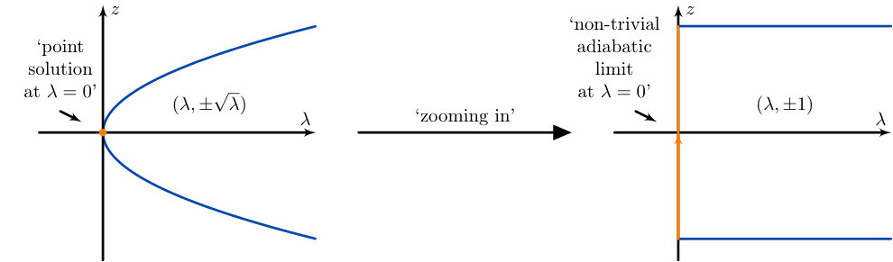 Figure 1
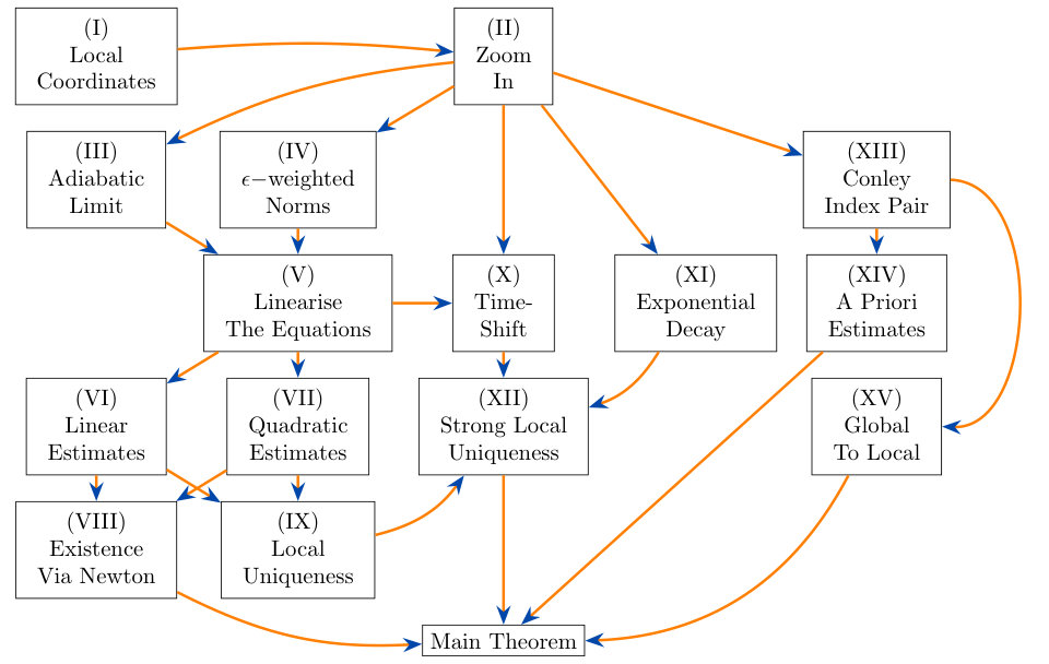 Figure 2
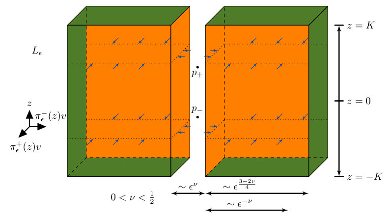 Figure 3
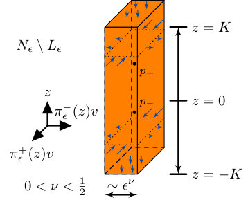 Figure 4