This paper investigates how the minimal surface area functional in hyperbolic 3-manifolds behaves under geometric convergence, focusing on the interaction with short geodesics and establishing continuity properties.
Contribution
It proves the lower semi-continuity and conditions for continuity of the minimal surface area functional in hyperbolic 3-manifolds, highlighting the role of short geodesics.
Findings
01
The functional is lower semi-continuous under geometric convergence.
02
Continuity holds when the minimal surface satisfies certain conditions.
03
Interaction between minimal surfaces and short geodesics is characterized.
Abstract
If M is a finite volume complete hyperbolic 3-manifold, the quantity A1(M) is defined as the infimum of the areas of closed minimal surfaces in M. In this paper we study the continuity property of the functional A1 with respect to the geometric convergence of hyperbolic manifolds. We prove that it is lower semi-continuous and even continuous if A1(M) is realized by a minimal surface satisfying some hypotheses. Understanding the interaction between minimal surfaces and short geodesics in M is the main theme of this paper
No public reviews on file for this paper yet. If you reviewed it on a platform where reviews are public (OpenReview, ICLR, NeurIPS, ICML), you can paste yours below so the community can read it here.
Videos
No videos yet. Explain this paper in a talk, walkthrough, or lecture? Add one.
Full text
Minimal surfaces near short geodesics in hyperbolic 3-manifolds
Laurent Mazet
Université Paris-Est, LAMA (UMR 8050), UPEC, UPEM, CNRS, 61, avenue
du Général de Gaulle, F-94010 Créteil cedex, France
If M is a finite volume complete hyperbolic 3-manifold, the quantity A1(M) is
defined as the infimum of the areas of closed minimal surfaces in M. In this paper we
study the continuity property of the functional A1 with respect to the geometric
convergence of hyperbolic manifolds. We prove that it is lower semi-continuous and even
continuous if A1(M) is realized by a minimal surface satisfying some hypotheses.
Understanding the interaction between minimal surfaces and short geodesics in M is the
main theme of this paper
1. Introduction
The area of a closed minimal surface Σ in a complete hyperbolic 3-manifold is
bounded above by −2πχ(Σ); this follows from the Gauss equation. Finding an
optimal lower bound for the area is a more subtle question. Notice that in dimension 2,
there is no lower bound for the length of a closed geodesic in a hyperbolic surface.
However the Margulis lemma and the monotonicity formula does give a lower bound of
2π(cosh(εˉ)−1), for the area of a properly immersed minimal surface in a
complete hyperbolic 3-manifold; εˉ is the Margulis constant. According to
explicit estimates of εˉ, this number is at least 0.104 [11].
In a previous paper the authors proved the area is at least 2π when Σ is a
closed embedded minimal surface in a complete finite volume hyperbolic 3-manifold of
Heegaard genus at least 6. If Σ is non-orientable the lower area bound is π.
Perhaps the main goal of the present paper it to introduce techniques to resolve the
remaining cases: 2≤Heegaardgenus≤5.
In our paper [10], we introduce the quantity A1(M), where M is a compact orientable 3-manifold. If O denotes
the collection of all smooth
orientable embedded closed minimal surfaces in M and U the collection of all
smooth non-orientable ones, A1(M) is defined by
[TABLE]
so A1(M) gives a lower bound for the area of any minimal surface in M.
The main result in [10] says that A1(M) is the area (or twice the area) of
some minimal surface in M. Moreover it gives some characterization of this minimal
surface in terms of its index and its genus.
Let (gi)i be a sequence of smooth Riemannian metrics on M which smoothly converge to
gˉ. Because of the characterization of the minimal surface that realizes
A1(M,gi) and thanks to a compactness result by Sharp [14], it can be proved
that liminfA1(M,gi)≥A1(M,gˉ).
Moreover, if A1(M,gˉ) is realized by a non degenerate minimal surface,
limA1(M,gi)=A1(M,gˉ). However one can produce examples where A1 is
not upper semi-continuous (F. Morgan suggested examples of a 2-sphere looking like a pear).
Concerning hyperbolic manifolds, our study proves that, if M is
hyperbolic and its Heegaard genus is at least 6, then A1(M)≥2π which
gives a universal lower bound for the area of a minimal surface in M. This reasoning can
be adapted to the case M is a finite volume hyperbolic manifold (not necessarily compact).
In order to remove the hypothesis about the Heegaard genus, we ask the question of the
continuity of A1 when the space of hyperbolic manifolds is endowed with the
geometric convergence topology. Here the situation is not as above where we have a
sequence of Riemannian metrics on a fixed manifold, here we have a sequence of manifolds Mi
with changing topologies.
Moreover, if (Mi)i is a non trivial converging sequence of
hyperbolic manifolds then Mi contains a geodesic γi whose length goes to [math].
As a consequence, an important question for our study is to understand the behaviour of a minimal
surface intersecting a neighborhood of a short geodesic.
This question has been already studied by several authors. For example, Hass [7]
and Huang and Wang [8] study the geometry of minimal surfaces near a short
geodesic in order to construct hyperbolic manifolds that fiber over the circle but such
that the fibers can not be made minimal.
Our study of minimal surfaces near short geodesics starts with a result of
Meyerhoff [11]. Basically it says that a short geodesic in M of length ℓ has
a embedded tubular neighborhood NRℓ of radius Rℓ and limℓ→0Rℓ=+∞.
We obtain two results concerning minimal surfaces in NRℓ. The first
one deals with stable minimal surfaces in tubular neighborhood of short geodesics
(Corollary 7).
Basically it says that such a stable minimal surface either stays far from the short geodesic
or it intersects transversely the short geodesic. Moreover in the second case, the surface
must have a very large area in the Rℓ tubular neighborhood of the geodesic.
Our second result deals with general minimal surfaces (not assumed to be
stable)
(Proposition 9). It says
that a minimal surface in the neighborhood of a short geodesic either stays very far from
the core geodesic or comes very close to it (the estimate depending on the index of the
minimal surface). As above in the second case, we obtain a
lower bound for the area of a minimal surface coming close to the short geodesic.
Actually these two results are very similar to results we obtained with Collin and Hauswirth
in [5] concerning the geometry of minimal surfaces in hyperbolic cusps. In
both cases, the argument is based on the fact that the tubular neighborhoods are foliated
by equidistant tori whose diameter are small. As a consequence, an embedded minimal surface
with bounded curvature can not be tangent to these equidistant surfaces.
Once the behaviour of minimal surfaces close to short geodesics is understood, we study the
continuity of A1. A version of our result can be stated as follows. It is similar to
the result that can be obtained for a fixed manifold with a converging sequence of
metrics.
Theorem**.**
Let Mi→M be a converging sequence of hyperbolic cusp manifolds. Then
[TABLE]
If A1(M) is not realized by the area of a stable-unstable separating minimal
surface, then
[TABLE]
Let us recall that ”stable-unstable” means that the first eigenvalue of the stability
operator is [math]. Of course one can expect that the surface that realizes A1(M) is never stable-unstable but we do not know how to prove this. Actually it is possible
to expect that no minimal surface in a hyperbolic manifold is stable-unstable. In fact
the above result is a combination of two
propositions: Propositions 22 and 25
The main difficulty in the proof of Proposition 25 is to be able to control
where is located a minimal surface Σi that realizes
A1(Mi). Actually, our study of minimal surfaces near short geodesics implies that
Σi can not enter into a tubular neighborhood of a short geodesic. So it stays in a
part of Mi where the convergence Mi→M is just the smooth convergence of
the metric tensor. Thus a compactness result by Sharp [14] gives the lower
semicontinuity of A1. Concerning Proposition 22, we first prove that
limsupA1(Mi) is bounded. Thus if A1(M) is not realized by a
stable-unstable separating minimal surface Σ then Σ can be deformed into a
minimal surface in Mi. This implies the second inequality.
Of course one can also think about hyperbolic manifolds with infinite volume and ask the following question.
For which class of complete hyperbolic 3-manifolds of infinite volume can one hope for an
area lower bound 2π? There may not exist a closed minimal surface in M, but if A1(M) is
realized, can one expect it to be at least 2π?
The paper is organized as follows. In Section 2.1, we recall some basic facts
about the description of cusp and tubular ends of complete finite volume hyperbolic
3-manifolds. Section 3 studies the geometry of minimal surfaces with bounded
curvature in tubular ends. In Section 4, we study the general
behaviour of minimal surfaces in tubular ends. In Section 5 we recall some
facts about the min-max theory for minimal surfaces that we will use in the next sections.
Section 6 is devoted to recall the work we made in [10] and how it
should be adapted to work with non compact hyperbolic manifolds. Sections 7
and 8 are devoted to the study of the lower and upper semi-continuity of
the A1 functional. Finally in Appendix A, we prove some technical
results and formulas.
Preliminary remarks
Let S be a smooth Riemannian surface, we will denote by ∣S∣ its area.
Let (T,dσ2) be a flat torus. Its universal cover is a flat R2 so we have
coordinates (x1,x2) such that the flat metric can be written dx12+dx22. Then T
is the quotient of R2 by some lattice Γ. We say that (x1,x2) is an orthonormal
coordinate system on T.
Moreover, we can choose (x1,x2) such that Γ is generated by v1,v2 where
v1=(a1,0) and v2=(a2,b2). We then say that (x1,x2) is a well oriented
orthonormal coordinate system.
We notice that if (T,dσ2) has diameter δ then the lattice can be generated
by vectors of length less than 2δ.
2. Hyperbolic manifolds
In this first section we recall some facts concerning the geometry of hyperbolic
3-manifolds with finite volume also called cusp manifolds. We refer to [2] for
part of this description.
2.1. The cusp and tubular ends
Let M be a complete hyperbolic 3-manifold of finite volume. For any
ε less than the Margulis constant, the manifold M can be split into two parts: the
ε-thick part M[ε,∞) which is connected, not empty (recall that p∈M[ε,∞) is any non null homotopic closed loop at p has length at least ε) and the ε-thin
part which may have a finite number of
connected components. The connected components of the thin part are of two types: cusp
ends and tubular neighborhoods of closed geodesics also called tubular ends.
Cusp ends are isometric to E0=T×R+ endowed with a metric
[TABLE]
where dσ2 is a flat metric on the 2-torus T. We define Et=T×[t,+∞).
We notice that if E0 is a component of the ε-thin part then Et is a component
of the the δε-thin part with e−2t≤δ≤e−t/2.
For tubular ends, let γ be a short geodesic in M and consider c a
lift of γ to H3. If R
is small the R-tubular neighborhood NR of γ in M is the quotient of the R
tubular neighborhood VR of c in H3 by some loxodromic transformation τ of
axis c (see Figure 1).
In order to introduce some coordinate system, let z denote arclength along c and let
ν(z),τ(z) be parallel orthogonal unit normal vectorfields along
γ, we introduce cylindrical coordinates in VR by
[TABLE]
In these coordinates, the hyperbolic metric is
[TABLE]
NR can be viewed as the quotient of MR={(t,θ,r)∈R2×[0,R]} by the
relations (t,θ,0)∼(t,θ′,0), (t,θ,r)∼(t,θ+2π,r) and
(t,θ,r)∼(t+ℓ,θ+α,r) for some parameters ℓ>0 and α. ℓ is
the length of the geodesic loop γ and α is called the twist
parameter of γ (it
is the angle of the loxodromic transformation). As above, if NR is a component of
the ε-thin part, then Nr is a component of the δε-thin part
some some δ∈[e2(r−R),e(r−R)/2] if R and r are larger than some
universal constant. In the following, we denote by Srˉ=∂Nrˉ the torus
{r=rˉ}.
The above coordinates are called tubular coordinates. In order to be
coherent with the coordinates we use on cusp ends, we will also use the coordinate system
(x1,x2,t)=(θ,z,R−r) such that the metric can be written
[TABLE]
on T×[0,R] where T is the quotient of R2 by the translations by (2π,0)
and (α,ℓ) (notice that g is singular on T×{R}).
The interest of these coordinates is that any part of a cusp or tubular end can be
described as T×[a,b] with some metric dσt2+dt2 where dσt2 is a
flat metric on the torus T. We denote by Tt=T×{t}. So the family (Tt)t
gives a foliation of the ends by tori.
If C is the torus in such an end that corresponds to T×{tˉ}, the graph of
a function u:Ω⊂C→R is just the surface parametrized by {(p,t)∈T×R∣t=tˉ+u(p)} (notice that we will often identify C⊂M with Ttˉ∈T×R).
One question is to know what is the maximal radius R that can be considered
in the above discussion (NR being embedded). This has been estimated by Meyerhoff in
[11] where the following result is proved.
Theorem 1**.**
Let γ be a geodesic loop in a complete hyperbolic 3-manifold. If the length ℓ
of γ is less than 4π3ln2(2+1), then there exists an
embedded tubular neighborhood around γ whose radius R satisfies
[TABLE]
where k=cosh34πℓ−1.
In the sequel we denote by Rℓ the solution of
sinh2R=21(k1−2k−1). When ℓ is small this implies that
sinh2Rℓ∼cosh2Rℓ∼4πℓ3. For example, the area of
SRℓ goes to 23 as ℓ→0.
Let us notice that the mean curvature of the torus Sr0 with respect to −∂r
is (tanhr0+cothr0)/2.
2.2. The geometric convergence
The space of cusp manifolds with volume less than V0 is compact for geometric
convergence. This convergence is defined as follows (see Sections E.1 and E.2 in
[2]). Let Πi:H3→Mi and Π:H3→M be the universal
covers and o a point in H3. We say that the pointed manifolds (Mi,Πi(o))
converge for the geometric convergence topology to (M,Π(o)) if, for any r,
there are fi:B(o,r)⊂H3→H3 which are
equivariant (Π(z)=Π(z′)⇔Πi(fi(z))=Πi(fi(z′)))
such that (fi)i converges to the identity in the C∞ topology (here B(o,r)
denotes the geodesic ball in H3). Actually defining φi by φi(Π(z))=Πi(fi(z)), we will often use the following consequence (see
Lemma E.2.2 in [2]).
Lemma 2**.**
Let (Mi)i be a sequence of finite volume hyperbolic manifolds converging to M
in the geometric topology. Let ε>0 be fixed, after eliminating some initial terms,
there exists:
•
(σi)i* with σi>0 and σi→0,*
•
(ki)i* with ki>1 and ki→1,*
•
for all i a ki-quasi-isometric embedding φi from a neighborhood of
M[ε,∞) into Mi.
with the following properties
•
φi(M[ε,∞))* is contained in the interior of Mi[ε−σi,∞) and*
•
φi(∂M[ε,∞))* does not meet an open neighborhood of
Mi[ε+σi,∞).*
Here ki-quasi isometry must be understood as smooth maps φi such that
[TABLE]
When we will use these properties, we will not forget that φi come from maps fi that
are C∞ close to id.
Actually, ε is always chosen small enough such that the ε-thin part of M contains only cusp ends. Moreover if ε is small enough each connected component of
Mi[ε−σi,ε+σi] contains exactly one component of φi(∂M[ε,∞)) (see Theorem E.2.4 in [2]). The description of this
component of φi(∂M[ε,∞)) is given by the following result.
Lemma 3**.**
Let (Mi)i, M, ε>0 and φi as above. Let C be a connected
component of ∂M[ε,∞). Then for i large, φi(C) is a
graph of a function ui
over the corresponding component Ci of ∂Mi[ε,∞). Moreover
ui→0 and C and Ci are κi-quasi-isometric with κi→1.
Proof.
C is a surface with principal curvatures 1. Thus φi(C) has principal curvatures
close to 1 and between 1/2 and 3/2.
Since φi(C)⊂Ai where Ai is a component of
Mi[ε−σi,ε+σi], φi(C) is contained either
in a cusp end of Mi or a neighborhood of a short geodesic of γi. In the second
case, there is a smallest δi≤σi such that φi(C)⊂Mi[ε−σi,ε+δi] so φi(C) is tangent to a
boundary torus of ∂Mi[εi+δi,∞). The comparison of the mean
curvature at this tangency point gives the mean curvature of ∂Mi[εi+δi,∞) is close to 1. Thus the distance from γi to
φi(C) is very large and goes to +∞.
In both cases, Ai is described as Ti×[−αi,βi] with a metric
dσi,t2+dt2 with αi,βi→0 and Ci=Ti×{0} is the boundary of
Mi[ε,∞) in Ai.
Let γ be a geodesic in φi(C). Since φi(C) has curvature uniformly bounded,
there is k0 such that ∣∂s(γ′(s),∂t)∣≤k0 so
∣(γ′(s),∂t)∣≥∣(γ′(0),∂t)∣/2 for
0<s<s0=∣(γ′(0),∂t)∣/(2k0). Looking at the t coordinate along γ,
we then have βi+αi≥∣t(γ(s0))−t(γ(0))∣≥4k0∣(γ′(0),∂t)∣2. Since αi+βi→0, this implies
that the angle between φi(C) and ∂t goes to π/2 uniformly. Since
φi(C) is embedded this implies that
φi(C) is a graph over Ci: there is a function ui:Ci→R
such that φi(C)={(p,t)∈T×R∣t=ui(p)}.
Since the angle between φi(C) and ∂t goes to π/2, the
gradient of ui goes to [math]. Besides φi(C)⊂Ai so ∣ui∣ is close to
[math].
This implies that (p,ui(p))∈φi(C)↦(p,0)∈Ci is
a κi-quasi-isometry (κi→1) which can be composed with φi:C→φi(C) to obtain a κiki-quasi-isometry.
∎
As consequence, we have the following result.
Corollary 4**.**
Let V0 be positive then there are ℓ0, δ0, s0 such the following is
true. Let M be a cusp manifold with volume less than V0 and γ be a geodesic
loop of length ℓ≤ℓ0. Then SRℓ=∂NRℓ has diameter less than δ0 and
systole larger than s0.
The set of flat tori with diameter less than δ0 and systole larger than
s0 is a compact subset of the set of flat tori.
Proof.
If it not true there is a sequence of cusp manifolds Mi that converge to M
and in Mi there is a geodesic loop γi of length ℓi→0 such that either the
diameter of SRℓi goes to ∞ or its systole goes to [math].
After taking a subsequence, we can assume that the tubular ends around γi
converges to one cusp end in M. Let ε>0 be small and consider C the
component of ∂M[ε,∞) inside this cusp end. Let Ci be the
component of ∂Mi[ε,∞) inside the tubular end around γi. By
the above lemma, C and Ci are 2 quasi-isometric. So the area Ci is close to that
of C. Since the area of SRℓi in Mi is close to 3/2 this
implies that the distance between Ci and SRℓi is uniformly bounded. Since
the diameter and the systole of SRℓi differ from those of Ci by at most
a uniform factor. This contradicts that either the diameter goes to ∞ or the
systole goes to [math].
∎
Remark 1*.*
Let us consider a particular one sided neighborhood of φi(C) in Mi.
Actually, let A be the part of the 2-tubular neighborhood of C
inside M[ε,∞). Thus φi(A) is a one sided
neighborhood of
φi(C).
A can be parametrized by T×[−2,0] with the metric
g=e−2tdσˉ2+dt2. Let X:T×[−2,0]→M be this parametrization
and (x1,x2) be orthonormal coordinates such that g=e−2x3(dx12+dx22)+dx32.
Let us now
estimate the metric φi∗gi. We notice that X lifts to an equivariant map
X:R2×[−2,0]→H3i.e.X=ΠX. If g~i=g~i,kldxkdyl we have
[TABLE]
since Πi is a local isometry. Since fi converges to the identity map in the
C∞ topology this implies that g~i→g in the
C∞ topology.
Remark 2*.*
The topology of a complete finite volume hyperbolic 3- manifold determines its
hyperbolic structure. Thus if a converging sequence Mi→M is not constant,
there is a subsequence whose topologies are distinct from that of M. then there
are short geodesics γi in Mi whose lengths converge to zero and whose maximal embedded
tubular neighborhoods are converging to cusp ends of M (see Figure 2).
3. Transversallity in tubular ends
The aim of this section is to understand the behaviour of a minimal surface in a tubular
end when we know a priori an upper bound on its curvature. A similar study was
made for cusp ends in [5].
In this section, we use the tubular coordinates (z,θ,r).
3.1. An intersection property
We recall that, if c is a geodesic in H3, Vr denotes its tubular neighborhood of
radius r. Moreover, for r>0, we denote Br=∂Vr.
Lemma 5**.**
Let k0 and ε0 be positive, then there are r0 and η0 such that the
following is true. Let
c be a geodesic in H3. Let r∈[0,r0] and pi=(zi,θi,r) (i=1,2) be
two points in Vr0 such that θ2∈[θ1+3π,θ1+32π] and
z2∈[z1−η0,z1+η0]. Let Σi, i=1,2 be surfaces in Vr0 whose
curvatures are bounded by k0, pi∈Σi and
dΣi(pi,∂Σi)>ε0. If both Σi are tangent to Br at
pi (if r=0 we assume moreover that a unit normal vector to Σi at pi is
∂r(zi,θi,0)) then Σ1 and Σ2 has non empty transversal
intersection.
Proof.
We look for r0≤2. In V2 the hyperbolic metric is cosh2rdz2+sinh2rdθ2+dr2. Let us change
the metric in V2 to the Euclidean metric ge=dz2+r2dθ2+dr2. So there are
constants k~0 and ε~0 depending only on k0 and ε0 such
that, with ge, Σ1 and Σ2 have curvature bounded by
k~0 and dΣi(pi,∂Σi)>ε~0.
Thus there is η1>0 such that Σi can be described as a graph over the Euclidean
disk of radius η1 tangent to Σi at pi (see Proposition 2.3 in
[13]). Moreover if η1 is chosen
small enough, the gradient of the function parametrizing Σi is less than
1/10.
Let r0=η0=η1/10. With these choices, the tangent disks of radius η1
tangent to Σi at pi must intersect at an angle between π/3 and 2π/3
(see the schematic figure 3). Moreover since each Σi is at a distance less
than η1/10 from its tangent disk, Σ1 and Σ2 must intersect and, as
the gradient is less than 1/10 and the angle between the disks is in [π/3,2π/3],
the intersection is transverse.
∎
3.2. The transversality result
The main result of the section is then the following. We recall that Sr=∂Nr.
Proposition 6**.**
Let δ0, k0 and ε0 be positive, then there is ℓ0>0 and R such that
the following is true. Let ℓ≤ℓ0 and NRℓ be the hyperbolic tubular neighborhood
of a geodesic loop γ of length ℓ and such that the diameter of
SRℓ is less than
δ0. Let Σ be an embedded minimal surface in NRℓ whose curvature is
bounded by k0. Let rˉ<Rℓ−R and p be a point in Σ∩Srˉ such that dΣ(p,∂Σ)>ε0. Then Σ is not tangent to
Srˉ at p.
We notice that for rˉ=0, Srˉ is just the central geodesic γ so the
proposition states that Σ can not be tangent to γ.
Proof.
We start with some ℓ0 such that Rℓ>10. Let r0≤1 and η0 be given by
Lemma 5 for k0 and ε0 (we assume ε0≤1). We first prove that the result is true if
rˉ≤r0.
Let Σ be a minimal surface as in the statement of the proposition and assume that
Σ is tangent at p to Sr for some r. We consider the lift
Σ of Σ to H3. Σ is then contained in a solid
cylinder VRℓ.
The surface Σ is then an embedded minimal surface (may be non connected) which is invariant by
the action of the loxodromic transformation τ:(z,θ,r)↦(z+ℓ,θ+α,r).
Let p1 be a lift of p. We can assume that p1=(0,0,rˉ); if rˉ=0, we assume that
∂r(0,0,0) is the unit normal vector to Σ.
SRℓ has a diameter less than δ0. So, for any q in BRℓ, the intrinsic
disk of radius δ0 in
BRℓ and center q must contain an image of (0,0,Rℓ) by some τn.
Let us consider the domain Ar={(z,θ,r)∈Br∣z∈[−coshRℓδ0,coshRℓδ0],θ∈[2π−sinhRℓδ0,2π+sinhRℓδ0]}, ARℓ is a square in
BRℓ whose
edges have length 2δ0.
So ARℓ contains an image of (0,Rℓ,0) by some τn. This implies that τn is
the composition of a vertical translation by some z′∈[−coshRℓδ0,coshRℓδ0] and a rotation by some θ′∈[2π−sinhRℓδ0,2π+sinhRℓδ0].
The point p2=τn(p1)=(z2,θ2,rˉ) is another lift of p in Arˉ.
Σ is then also tangent to Brˉ at p2. We have
∣θ2−π/2∣≤δ0/sinhRℓ and ∣z2∣≤δ0/coshRℓ. So we can choose
ℓ0 such that, for ℓ≤ℓ0, δ0/sinhRℓ≤π/6 and δ0/coshRℓ≤η0. Then we can apply Lemma 5 to the geodesic disks Σi of radius
ε0 in Σ around pi. Lemma 5 applies since, when
rˉ=0, the unit normal vector to Σ2 at p2 is
∂r(z2,θ2,0) with ∣θ2−π/2∣≤δ0/sinhRℓ (Σ2 is the
image of Σ1 by τn). This gives that Σ has
transverse self-intersection which is impossible. So the result is proved for rˉ≤r0.
Let us now prove that we can extend this result to the region r0≤rˉ≤RL−R for some R>0.
If the result is not true, for any n>0, we can find a neighborhood NRℓn of a closed
geodesic γn of length ℓn≤n1 and a minimal surface
Σn in NRℓn which is tangent to Srn at pn for some rn≤Rℓn−41lnn (notice that Rℓn−41lnn>0).
Actually because of the first part we can assume rn>r0. In the following we
denote Rℓn by Rn.
Let η1=min(r0/10,η0) and replace the sequence Σn by the sequence of
η1-geodesic disks in Σn centered at pn. So we can be sure that Σn
never touches the central geodesic γn and stays outside of Nr0−η1.
We lift Σn to MRn endowed with the metric (1). This
gives us a minimal surface Σn which is doubly periodic and may be non
connected. Σn is doubly periodic by translation in the (z,θ)
parameters by two vectors v1n,v2n. Since TRn has diameter less than δ0
we can choose v1n,v2n of Euclidean length less than sinhRnδ0.
The point pn lifts to some point p~n whose coordinates can be assumed to be
(0,0,rn) where rn∈(r0,Rn−21lnn). We can assume that either rn
converges to some rˉ or to ∞. In the first case the ambient space around
(0,0,rˉ) is M∞=R2×(0,+∞) with the
metric (1). If rn→∞, we make the following change of coordinates a=ernz, b=ernθ and ρ=r−rn. So the ambient space is now
R2×(r0−η1−rn,Rn−rn) with the metric
[TABLE]
As n goes to +∞, these metrics converge smoothly to 4e2ρ(da2+db2)+dρ2 on R3. In this model, the vectors v1n,v2n become ernv1n and ernv2n whose lengths are less that sinhRnδ0ern=O(ern−Rn)=O(e−21lnn)→0.
Actually, the cases rn→rˉ and rn→+∞ are very similar. Let us look first at
the case rn→rˉ. We notice that the metric satisfies the hypotheses of
Lemma 26 (Appendix A.1) for some parameter A and for
r∈[rˉ−η1,Rn]: we have x1=z, x2=θ, x3=r and h=sinh.
So there is a C and a function un defined on the Euclidean
disk {(z,θ)∈R2∣z2+θ2≤2C2/sinh2rn} such that (z,θ)↦(z,un(z,θ),θ) is a parametrization of a neighborhood of p~n in
Σn. Moreover we have un(0,0)=rn, ∇un(0,0)=0 and the estimates
[TABLE]
Here ∇ denote the Euclidean gradient operator.
So the sequence un is uniformly controlled in the C2 topology and moreover un
solves the minimal surface equation (2). Thus, after considering a subsequence, un converges
to some u defined on Drˉ={(t,θ)∈R2∣t2+θ2≤sinh2rˉ2C2} which solves the minimal surface equation.
If rn→+∞, we apply the change of variables a=ernt,
b=ernθ and ρ=r−rn. So we get a new function
wn(a,b)=un(e−rna,e−rnb)−rn
defined on {(a,b)∈R2∣a2+b2≤sinh2rn2C2e2rn}. As above wn
satisfies the estimates
[TABLE]
and solves a minimal surface equation (2). So we can assume it converges to some function w
defined on Δ={(a,b)∈R2∣a2+b2≤4C2}.
Let us denote the surface {r=R} by PR. The surface Σn is doubly
periodic so it is tangent to Prn at any point of the form (0,0,rn)+kv1n+lv2n
for (k,l)∈Z2. Moreover, around these points, it is parametrized locally on
Drn+kv1n+lv2n by (z,θ)↦(z,un,k,l(t,θ),θ) where
un,k,l(z,θ)=un((z,θ)−kv1n−lv2n). The surface Σn is
embedded, this implies that un≤un,k,l or un≥un,k,l on Dn∩(Dn+kv1n+lv2n) if it is non empty (notice that we can have un≡un,k,l on
the intersection).
If rn→rˉ, let v0 be a vector in Drˉ. Since vin→0, there are
sequences (kn)n and (ln)n such that knv1n+lnv2n→v0. As n→∞,
the sequence of functions un,kn,ln then converges to uv0 on Drˉ+v0
where uv0(⋅)=u(⋅−v0). Because of un≤un,k,l or un≥un,k,l, we get u≤uv0 or u≥uv0 on Drˉ∩(Drˉ+v0).
If rn→∞, we can do the same with the change of coordinates since
ernvin→0. So for any v0∈Δ, we have w≤wv0 or
w≥wv0 on Δ∩(Δ+v0) where
wv0(⋅)=w(⋅+v0).
We now consider the case rn→rˉ (the second one is similar). Let G be the
totally geodesic surface in M∞ tangent to Prˉ at (0,rˉ,0). As
Σ, G can be described as the graph of a function h over Drˉ.
We have h(0)=rˉ and there is some α>0 such that, over Drˉ,
h(z,θ)≥rˉ+α(z2+θ2). This second property comes from the fact that
the principal curvatures of Prˉ with respect to ∂r are −tanhrˉ<0
and −cothrˉ<0. The functions u and h are two solutions of the minimal surface
equation (2) with the same value and the same gradient at the origin. So by Bers theorem, the function u−h
looks like a harmonic polynomial of degree at least 2.
If the degree of the polynomial is 2, on can find v0∈Drˉ∖{(0,0)} such that
(u−h)(v0)>0 and (u−h)(−v0)>0. Then we have
[TABLE]
So this contradicts u≤uv0 or u≥uv0 on the whole Drˉ∩(Drˉ+v0)
If the degree is at least 3, the growth at the origin of h implies that u≥rˉ
on a smaller disk D′⊂Drˉ and u>rˉ on D′∖{(0,0)}. So if
v0∈D′∖{(0,0)} we have
[TABLE]
Once again, this contradicts u≤uv0 or u≥uv0 on the whole Drˉ∩(Drˉ+v0)
If rn→∞, the same argument can be done with a totally geodesic surface tangent to
the horosphere.
∎
3.3. A first area estimate
The preceding result allows us to estimate the area of a minimal surface with bounded curvature in a tubular end.
Corollary 7**.**
Let δ0 and k0 be positive, then there is ℓ0 and R such
that the following is
true. Let ℓ≤ℓ0 and NRℓ be the hyperbolic tubular neighborhood
of a geodesic loop γ of length ℓ and such that the diameter of
SRℓ is less than
δ0. Let 0<R≤Rℓ−R and Σ be a compact embedded
minimal surface in NR+1
whose curvature is bounded by k0 and ∂Σ⊂SR+1. Then one of the
following possibilities occurs
(1)
Σ∩NR=∅**
2. (2)
Σ∩NR* is a finite union of minimal disks. Each of these disks
has boundary curve homotopic to a parallel of SR=∂NR and ∣Σ∩NR∣≥2π(coshR−1).*
A parallel of SR is a curve {z=const.} in the tubular coordinates.
Proof.
Let ℓ0 and R be given by Proposition 6 for δ0, k0
and ε0=1.
Let Σ be as in the statement of the corollary and assume Σ∩NR=∅. By Proposition 6, Σ is transverse to
the foliation (Sr)r of NR. So any connected component of Σ∩NR intersects the geodesic loop γ transversely. This implies that in
Nε for ε small each connected component of Σ∩Nε is a disk
whose boundary is homotopic to a parallel. Thus this description extends by
transversality to Σ∩NR. Let Π be the geodesic projection from
NR to a geodesic parallel disk Δ (i.e. the map (z,θ,r)↦(z0,θ,r) for some z0). This map is a contraction mapping and it is surjective on
any disk component of Σ∩NR since the boundary of such a disk is homotopic to a
parallel. As a consequence the area of such a disk component is at least that of Δ,
i.e.2π(cosh(R)−1).
∎
4. A maximum principle
One aim of this section is to study some aspect of the behavior of minimal surfaces
in a tubular end. Actually we need to study this in a more general setting. So we consider
the ambient space C=T×[a,b] endowed with some reference metric g=h2(x3)dσˉ2+dx32 where dσˉ2 is a
flat metric on the torus T.
We consider orthonormal coordinates (x1,x2) on T associated to dσˉ2; so gˉ=h2(x3)(dx12+dx22)+dx32.
On C, we also consider a second metric
g=akl(x1,x2,x3)dxkdxl. For s∈[a,b],
we denote Cs=T×[s,b]
and Ts=T×{s}. We are going to make several hypotheses on the metrics
gˉ and g. In order to formulate them, we need the following notation:
for k1,k2,k3,k4,k5∈{1,2,3} and p≤5, we define
[TABLE]
The hypotheses on gˉ and g are: there is A≥1 such that
H1
A21gˉ≤g≤A2gˉ
H2
h∣h′∣≤A, h∣h′′∣≤A and h∣h′′′∣≤A.
H3
∣akl∣≤Ahn2(k,l)(x3), ∣∂iakl∣≤Ahn3(k,l,i)(x3),
∣∂i∂jakl∣≤Ahn4(k,l,i,j)(x3) and ∣∂i∂j∂makl∣≤Ahn5(k,l,i,j,m)(x3).
H4
h′≤0 and the mean curvature vector of Ts with respect to g points in the
∂x3 direction (this is also true for the metric gˉ since h′≤0)
One consequence of H1 and H2 is that the sectional curvatures of gˉ are uniformly
bounded. Actually by H1 and H3 the sectional curvatures of g are also uniformly
bounded. We also notice that these hypotheses does not depend on the choice of the
orthonormal coordinates on (T,dσˉ2).
4.1. The maximum principle
We have the following maximum principle for embedded minimal surfaces in C endowed
with the metric g.
Proposition 8**.**
Let i0∈N, then there is h0 such the following is true. Assume that
h(a)≤h0 and let Σ be an embedded minimal surface in
(C,g) whose non empty boundary is inside Ta and its index is less than i0. Then
Σ∩Ca+1/2=∅.
We notice that h0 will depend on i0, A and the metric dσˉ2. We
also notice that this control on h is actually a control on the size of the torus Ta.
Proof.
If the proposition is not true there is a sequence of function hn with hn(a)→0
and a minimal surface
in Sn∈(C,gn) (gn=an,kl(x1,x2,x3)dxkdxl)
such that ∂Sn⊂Ta, its index is less than i0 and Σ∩Ca+1/2=∅.
Let sn be the maximum of the x3 coordinate on Sn, x3≥a+1/2.
Let us define λn=(hn(sn))−1. Then we change the coordinates by
y1=x1, y2=x2 and y3=λn(x3−sn) and blow up the metric by a factor
λn.
This gives us a minimal surface Σn in
T×[λn(a−sn),0] that touches T0 and with boundary in
Tλn(a−sn) (we notice that λn(a−sn)→−∞). The ambient
metric is then g~n=bn,kl(y1,y2,y3)dykdyl where
[TABLE]
The reference metric becomes
[TABLE]
Because of the hypothesis H2, considering a subsequence, this metric converges to
the flat metric dσˉ2+dy32 in C2,α topology. Because of H3,
considering a new subsequence, the metrics g~n converges to a flat metric
hˉ=bˉkldykdyl in C2,α topology. For example we have
[TABLE]
So
[TABLE]
Once this is known, the arguments in order to conclude use the fact that Σn
converges to a minimal lamination in T2×R− endowed with the flat metric hˉ : the precise argument can be found in the proof of Proposition 1 in
[4].
∎
Remark 3*.*
We notice that h0 can be chosen uniformly if dσˉ2 lies in a compact
subset of flat metrics on T.
4.2. Some applications
In this section, we will see some consequences of the above result.
The case of cusp ends E=T×R+ endowed with gˉ=e−2x3dσˉ2+dx32 is the
simplest one. Indeed in this case the metric g is the reference metric gˉ.
Let L be fixed and replace x3↦e−x3 by some non increasing function h
such that h(x3)=e−x3 on [0,L] and h(x3)=e−(L+1/2) for x3>L+1. Then all the
above hypotheses H2,H4 are satisfied (the constant A can be chosen independently of L). So
Proposition 8 yields: if ∂E has small diameter, then no compact
embedded minimal surface with boundary inside ∂E and index less
than 1 can enter in E1/2. As a
consequence, in a cusp manifold M, there is ε>0 such that any compact embedded
minimal surface in M less than 1 is contained in M[ε,∞).
The second case of interest concerns the tubular ends.
Proposition 9**.**
Let K be a compact set of flat tori T. Then there are ℓ0 and R such
the following is
true. Let ℓ≤ℓ0 and NRℓ be a hyperbolic tubular neighborhood of a
geodesic loop of length ℓ such that SRℓ belongs in K. Let 0<R≤Rℓ−R and Σ be a compact embedded minimal
surface in NR+1 with ∂Σ∈SR+1 with index less than 1. Then one
of the following possibilities occurs
(1)
Σ∩NR=∅**
2. (2)
Σ∩N1=∅**
Moreover there is a universal constant κ such that, in the second case and for any
3≤R≤Rℓ−R,
∣Σ∩NR∣≥κs0eR−Rℓ where s0≤1 is a lower bound on the
systole of TRℓ.
Proof.
We first prove that Σ∩NR=∅ or Σ∩N1=∅. We have
seen in Section 2.1 that we can consider, on NRℓ, a coordinate system C=T×[0,Rℓ)
endowed with the metric g=sinh2(Rℓ−x3)dx12+cosh2(Rℓ−x3)dx22+dx32
((x1,x2) are orthonormal coordinates on T).
In order to fit with the notations of the preceding section we should introduce the
coordinates yi=sinh(Rℓ)xii=1,2 and y3=x3. The first two are orthonormal
coordinates on (T,dσˉ2)=sinh(Rℓ)2(dx12+dx22). So we define
gˉ=h2(x3)(dy12+dy22)+dy32 with h(x)=sinh(Rℓ−x)/sinh(Rℓ) and in these
coordinates the metric g can be written
[TABLE]
There is
A>0 (that does not depend on ℓ) such that
g and gˉ satisfy hypotheses H1, H2, H3 and H4 on T×[0,Rℓ−21).
Moreover we notice that, since SRℓ belongs to K, (T,dσˉ2)
belongs to a compact set of flat tori.
Let h0 be given by Proposition 8 and let R
be such that sinh(Rℓ−R)≤h0sinh(Rℓ). Consider 0<R≤Rℓ−R
and let Σ be an embedded minimal surface in NR+1∖N21
with ∂Σ∈SR+1 and index less than 1.
If Σ∩N1=∅, Σ can be seen as a minimal surface in (C,g)
with boundary in Ts where s=Rℓ−(R+1). Since h(s)≤h0,
Proposition 8 gives Σ∩Cs+1/2=∅. So in the tubular coordinates, we have Σ∩NR=∅.
In the second case we now prove the area estimate. For this we use the tubular
coordinates. We notice that Σ must meet all the tori Sr for 1≤r≤R+1.
Since g≤cosh2r(dz2+dθ2)+dr2 and the systole of TRL is at least
s0, the disk {(z+z0,θ+θ0,Rℓ)∣z2+θ2≤4cosh2Rℓs02} is embedded in SRℓ for any
t0,θ0. For any ρ∈[3/2,Rℓ], let us define a=coshRℓsinhρ4s0≤41. The cylinder Yρ={(z+z0,θ+θ0,r)∣r∈[ρ−2a,ρ] and z2+θ2≤4cosh2Rℓs02} is embedded in Nρ. Yρ
contains the geodesic ball of center (z0,θ0,ρ−a) and radius a which is then
embedded in Nρ. Indeed, in the cylinder, we have
[TABLE]
So the geodesic ball is contained in {(z+z0,θ+θ0,r+ρ−a)∣41sinh2ρ(z2+θ2)+r2≤a2} which is a subset of Yρ.
Since Σ meets any Sr for r≥1, for any ρ we can select z0,θ0
such that (z0,θ0,ρ−a)⊂Σ. So by the monotonicity formula in H3,
∣Σ∩Yρ∣≥πa2. We are going to sum over all these contributions to
estimate the area of Σ.
Let c(s)=(z(s),θ(s),Rℓ) be a parametrization of a systole of SRℓ and
consider the surface S in NRℓ parametrized by X:(s,r)∈S1×[1,Rℓ]↦(z(s),θ(s),r). So, for ρ1<ρ2, we can estimate
[TABLE]
So in Nρ∖Nρ−2a
[TABLE]
for some universal constant κ and κ′.
So considering a disjoint union of Nρ∖Nρ−2a in NR∖N1 that
covers NR∖N3/2, we obtain
[TABLE]
for any R≥3 and some universal constant κ′′′.
∎
5. The min-max theory
In this section we recall some definitions and results of the min-max theory for minimal
surfaces. There are basically two settings for this theory: the discrete and the
continuous one. We recall the main points that we will use in the sequel.
5.1. The discrete setting
The discrete setting for the min-max theory was developed by Almgren and Pitts (see
[1, 12]).
Let M be a compact orientable 3-manifold with no boundary. The Almgren-Pitts min-max theory
deals with discrete families of elements in Z2(M)i.e. integral rectifiable
2-currents in M with no boundary.
If I=[0,1], we define some cell complex structure on I and I2.
Definition 10**.**
Let j be an integer. I(1,j) is the cell complex on I whose [math]-cells are points
[3ji] and 1-cells are intervals [3ji,3ji+1].
The cell complex I(2,j) on I2 is I(2,j)=I(1,j)⊗I(1,j).
For these cell complexes we can associate some notations
•
I(m,j)0 denotes the set of [math]-cells of I(m,j).
•
I0(1,j) denotes the set of [math]-cells [0],[1].
•
The distance between two elements of I(m,j)0 is
[TABLE]
•
The projection map n(i,j):I(m,i)0→I(m,j)0 is defined by n(i,j)(x)
is the unique element in I(m,j)0 such that
[TABLE]
Let φ:I(m,j)0→Z2(M) be a map. The fineness of φ is defined by
[TABLE]
where M is the mass of a current.
We write φ:I(1,j)0→(Z2(M),{0}) to mean φ(I(1,j)0)⊂Z2(M) and φ(I0(1,j))={0}.
Definition 11**.**
Let δ be positive and φi:I(1,ki)0→(Z2(M),{0}) for i=1,2.
φ1 and φ2 are 1-homotopic in (Z2(M),{0}) with fineness δ if
there is k3∈N, max(k1,k2)≤k3 and a map
[TABLE]
such that
•
f(ψ)≤δ;
•
ψ([i−1],x)=φi(n(k3,ki)(x))* for x∈I(1,k3)0;*
•
ψ(I(1,k3)0×{[0],[1]})=0.
The main objects in the discrete min-max theory are the (1,M)-homotopy sequences.
Definition 12**.**
A (1,M)-homotopy sequence of maps into (Z2(M),{0}) is a sequence of maps {φi}i∈N,
[TABLE]
such that φi is 1-homotopic to φi+1 in (Z2(M),{0}) with fineness
δi and
•
limi→∞δi=0;
•
supi{M(φi(x)),x∈I(1,ki)0}<+∞.
Moreover we have a notion of discrete homotopy between (1,M)-homotopy sequences
Definition 13**.**
Let Sj={φij}i∈N (j=1,2) be two (1,M)-homotopy sequences of maps into
(Z2(M),{0}). S1 is homotopic to S2 if there is a sequence
{δi}i∈N such that
•
limδi=0;
•
φi1* is 1-homotopic to φi2 in (Z2(M),0) with fineness δi.*
This notion defines an equivalence relation between (1,M)-homotopy sequences. The set
of equivalence classes is denoted by π1#(Z2(M),M,{0}). The Almgren-Pitts
theory says that π1#(Z2(M),M,{0}) is naturally isomorphic to the homology
group H3(M,Z) (see Theorem 4.6 in [12] and [1]). We denote by ΠM the
element of π1#(Z2(M),M,{0}) that corresponds to the fundamental class in
H3(M). If S∈ΠM we say that S is a discrete sweep-out of M.
For S={φi}i a (1,M)-homotopy sequence we define
[TABLE]
If Π∈π1#(Z2(M),M,{0}) is an equivalence class, we define the width associated to Π by
[TABLE]
For Π=ΠM, the number WM=W(ΠM) is call the width of the manifold M. The
Almgren-Pitts theory says that this number is positive and is L(S) for some particular
S∈ΠM. If S={φi}i we say that φij(xj)j (xj∈I(1,kij)) is a min-max sequence if M(φij(xj))→WM.
Let M be a closed 3-manifold, then there is S={φi}i∈ΠM with
L(S)=WM and a min-max sequence {φij(xj)}j that converges (in the varifold
sense) to an integral varifold whose support is a finite collection of embedded connected
disjoint minimal surfaces {Si}i of M. So there are positive numbers {ni}i
such that
[TABLE]
A consequence of this result is that there is always a minimal surface S in M such
that ∣S∣≤WM. Actually, Zhou [16] proved that, if
Si is a non orientable minimal surface produced by the above theorem, then ni is
even.
5.2. The continuous setting
The continuous setting was developed by Colding and De Lellis [3]. Here we present it
with the modifications made by Song in [15].
Let M be Riemannian 3-manifold and consider N⊂M a bounded open subset
whose boundary ∂N, when non empty, is a rectifiable surface of finite
H2-measure. Moreover when ∂N=∅, we assume that each connected component C
of
∂N separates M.
If a<b∈R, we then have the following definitions.
Definition 15**.**
A family of H2-measurable closed subsets {Γt}t∈[a,b] in N∪∂N with finite H2-measure is called a generalized smooth family if
•
for each t there is a finite set Pt∈N such that Γt∩N is a smooth
surface in N∖Pt or the empty set;
•
H2(Γt)* depends continuously in t and t↦Γt is continuous
in the Hausdorff sense;*
•
on any U⊂⊂N∖Pt0, Γtt→t0Γt0 smoothly in U.
We notice the smoothness hypothesis is only made on Γt∩N so this allows
∂N to be non smooth. We now define the notion of continuous sweep-out in this
setting.
Definition 16**.**
If ∂N=∅, a generalized smooth family {Γt}t∈[a,b] is
called a continuous sweep-out of N if there exists a family of open subsets
{Ωt}t∈[a,b] of N such that
(sw1)
(Γt∖∂Ωt)⊂Pt* for any t;*
(sw2)
H3(Ωt△Ωs)→0* as t→s (where △
denotes the symmetric difference of subsets).*
(sw3)
Ωa=∅* and Ωb=N;*
If ∂N=∅, for a open subset Ω⊂N we denote
∂∗Ω=∂Ω∩N. A continuous sweep-out of N is then required to satisfy
(sw1) and (sw2) above except that ∂ is replaced by ∂∗ and t>a in (sw1). Moreover (sw3) is replaced by
(sw3’)
Ωa=∅, Ωb=N, Σa=∂N and Σt⊂N for t>a.
For a continous sweep-out as above {Γt}t∈[a,b], we define the quantity
L({Γt})=maxt∈[a,b]H2(Γt). When ∂N is a smooth
surface, constructing a continuous sweep-out can be done in the following way. Let f:N→[0,1] be a Morse function such that {f−1(0)}=∂N. Then if
Γt=f−1(t) for t∈[0,1], {Γt}t∈[0,1] is a sweep-out of N.
Two continuous sweep-outs {Γt1}t∈[a,b] and {Γt2}t∈[a,b] are said to
be homotopic if, informally, they can be continuously deformed one to the other (the precise
definition is Definition 8 in [15]). Then a family Λ of sweep-outs is called
homotopically closed if it contains the homotopy class of each of its elements. For such a
family Λ, we can define the width
associated to Λ as
[TABLE]
As in the discrete setting this number can be realized as the mass of some varifold supported by
smooth disjoint minimal surfaces (see Theorem 12 in [15]).
5.3. From continous to discrete
In order to construct discrete sweep-outs of a closed orientable 3-manifold M, we will use a result obtained by
Zhou (see Theorem 5.1 in [17]). We denote by C(M) the space of subsets in M
with finite perimeter. Let F denote the flat metric on Z2(M).
Theorem 17**.**
Let Φ:[0,1]→(Z2(M),F) be a continuous map such that
•
Φ(0)=0=Φ(1);
•
Φ(x)=∂[[Ωx]], Ωx∈C(M) for all x∈[0,1];
•
M0=∅* and M1=M*
•
supxM(Φ(x))<+∞.
Then there exists a discrete sweep-out S such that
[TABLE]
Here [[Ω]] denotes the element of Z3(M) corresponding to Ω.
Let us notice that if {Γt}t∈[0,1] is a continuous sweep-out of a compact orientable
Riemannian 3-manifold then Φ:t↦[[Γt]]∈Z2(M) satisfies the
hypotheses of the above theorem (as above [[Γt]] denotes the element of
Z2(M) corresponding to Γt).
6. The quantity A1(M)
In this section we recall some results the authors obtained in [10] (see also
[4]).
6.1. The quantity A1(M) for compact M
If M is a closed orientable Riemannian 3-manifold, we denote by O the collection of all smooth
orientable embedded closed minimal surfaces in M and U the collection of all
smooth non-orientable ones. We then define
[TABLE]
One of the results of [10] is the following theorem (Theorem B in [10])
Theorem 18**.**
Let M be an oriented closed Riemannian 3-manifold. Then A1(M) is equal to
one of the following possibilities.
(1)
∣Σ∣* where Σ∈O is a min-max surface of M associated to the
fundamental class of H3(M), Σ has index 1, is separating and A1(M)=WM.*
2. (2)
∣Σ∣* where Σ∈O is stable.*
3. (3)
2∣Σ∣* where Σ∈U is stable and its orientable 2-sheeted
cover has index [math].*
Moreover, if Σ∈O satisfies ∣Σ∣=A1(M), then Σ is of type 1 or
2 and if Σ∈U satisfies 2∣Σ∣=A1(M), then Σ is of type 3.
Actually in [10], the case (3) mentions the possibility for the orientable
2-sheeted cover to have index [math] or 1. In fact, the index 1 case can be ruled out
thanks to the work of Ketover, Marques and Neves [9].
If S denotes the collection of all smooth embedded stable minimal surfaces, we define
AS(M)=inf({∣Σ∣,Σ∈O∩S}∪{2∣Σ∣,Σ∈U∩S}). Actually we proved in [10] that
A1(M)=min(WM,AS(M)). In order to simplify some notations, we will denote
a(Σ)=∣Σ∣ if Σ∈O and a(Σ)=2∣Σ∣ is Σ∈U.
When M is not compact, one can still define O and U for M by considering
only compact embedded minimal surfaces in M. Of course these collections could be empty
but if its not A1(M) is well defined. If M is a cusp manifold this can be done.
6.2. The filler
We want to study A1(M) when M is a cusp manifold. In order to do that the idea is
to change M into a compact manifold D(M) that contains all the compact minimal
surfaces of M. To do this the main tool are the fillers.
Definition 19**.**
Let (T,dσ2) be a flat torus and L>10 be a real number. A filler F associated to
T and L is a solid torus endowed with a Riemannian metric g with the following
properties.
(i)
Let Tt be the set of points at distance t from ∂F. For t∈[0,L+1),
Tt is a smooth flat torus and TL+1 is a closed geodesic.
(ii)
The diameter of Tt is a decreasing function and the mean curvature vectors points
in the ∂t direction.
(iii)
For t∈[0,1], Tt has the metric e−2tdσ2.
(iv)
Any minimal surface Σ that meets all the Tt for 0≤t≤L−1
has area at least κL where κ is a constant depending on the systole of
(T,dσ2).
Proposition 20**.**
Let (T,dσ2) be a flat torus and L>10. There exists a filler associated to T
and L. Moreover, let δ and s be the diameter and the systole of
(T,dσ2) and K≤s/δ. Then there is δ0>0 that depends only on
K such that
(v)
if δ is less than
δ0, then any minimal surface Σ with ∂Σ⊂∂F
and index at most 1 satisfies
either Σ∩T1=∅ or Σ∩Tt=∅ for any t≤L−1.
Proof.
We construct F as T×[L+1] with a Riemannian metric
which is singular on TL+1=T×{L+1} in order for TL+1 to be a geodesic. We
use the notation Ft=T×[t,L+1].
Let f:[0,L+1]→R be a function satisfying the following properties
•
f(t)=t on [0,1],
•
f′>0 on [0,L+2/3) and f′=0 on [L+2/3,L+1].
•
f≤3.
•
f′ and f′′ are bounded independently of L.
On F∖FL, we define the metric g=e−2f(t)dσ2+dt2. Since f(t)=t on
[0,1], (iii) is satisfied.
In order to define the metric on FL, we consider a well oriented orthonormal coordinate system on
(T,dσ2) such that T is the quotient of R2 by the translations by (α,0) and
(β,ℓ).
Let η:[0,1]→[0,1] be a non increasing function such that η is decreasing on
[1/2,1], η=1 near [math], and η(x)=(1−x)α2πef(L+1) near 1. On
FL we extend the definition of the metric g by
[TABLE]
Since η(1)=0, the metric is singular at t=L+1. Let D be the unit disk and consider
the solid torus T constructed as the quotient of D×[0,ℓ] by the relation
(p,0)∼(Rβ(p),ℓ) where Rβ is the rotation of angle β. If
(ρ,θ) are the polar coordinates on D and h:T→FL is the map
(ρ,θ,z)↦(2παθ,v,L+1−ρ) the metric h∗g is given by
[TABLE]
so, near ρ=0 (i.e.t=L+1), it is equal to
h∗g=ρ2dθ2+e−2f(L+1)dz2+dρ2 which is a smooth metric on T near the
core circle {ρ=0}. So F is a smooth solid torus with a smooth metric and (i) is satisfied.
Because of the monotonicity of f and η, (ii) is satisfied. Moreover the curvature
of g is uniformly controlled on F∖FL. If ρ0 is the minimum of 1 and
half the systole of (T,dσ2), then for any p∈F1∖FL−1 the geodesic
ball of center ρ and radius e−3ρ0 is embedded in F∖FL.
Let Σ be a minimal surface that meets all the Tt for t∈[0,L]. Consider
tn=1+2e−3ρ0n and, for any n∈{0,…,n0} where tn0≤L+2≤tn0+1, let pn be in Ttn with pn∈Ttn∩Σ. Then by the
monotonicity formula, the area of Σ in the ball of radius e−3ρ0 and center
pn is at least ce−6ρ02 for some universal constant c. Since these balls are
disjoint, the area of Σ in F∖FL is at least
[TABLE]
if L≥10 and where κ only depends on the systole of (T,dσ2).
For item (v), we notice that (T,δ21dΣ2) belongs to a
compact subset of flat tori fixed by K. So Proposition 8 applies to
(F∖FL,δ2e−2f(t)δ2dσ2+dt2) to prove that if
Σ has index at most 1 and Σ⊂T×[0,,L−1] then
Σ⊂T×[0,1].
∎
6.3. The quantity A1(M) for cusp manifolds
In this section we recall the study of compact minimal surfaces inside orientable cusp manifolds we
made in [5, 10].
Let M be a cusp manifold. First we prove that M contains a compact embedded minimal
surface. Let ε be such that the ε-thin part is only made of cusp ends. Since
∂M[ε,∞) is smooth there is a homotopically closed family Λ of
sweep-outs associated to a Morse function on M[ε,∞) (we recall that the tori components of ∂M[ε,∞) are leaves of the sweep-outs). If ε′<ε,
M[ε′,ε] is foliated by tori that can be used to extend any continuous sweep-out
in Λ into a sweep-out of M[ε′,∞) that belongs to a homotopically
closed
family Λ′. Since W(M[ε,∞),∂M[ε,∞),Λ)≥∣∂M[ε,∞)∣ we obtain
[TABLE]
So there is W0>0 such that W0≥W(M[ε,∞),∂M[ε,∞),Λ) for any ε. Besides a continuous sweep-out of
M[ε,∞) must sweep out also a fixed geodesic ball in M. So there is w0
such that W(M[ε,∞),∂M[ε,∞),Λ)≥w0 for any
ε.
Thus we can choose ε small such that any flat tori C in ∂M[ε,∞) has small diameter and
w0>∣∂M[ε,∞)∣.
For each C, we consider a
filler FC
associated to the flat torus C and L that will be chosen later. ε is chosen small
enough such that item (v) of Proposition 20 is satisfied. Since there are a finite
number of C, item (iv) of Definition 19 gives some constant κ>0
independent of C. Then L is chosen such that κL≥W0+1.
We can glue each
filler FC along C to obtain a compact manifold without boundary denoted D(M) with
some metric. The construction of D(M) depends on two parameters ε and L, so
sometimes we will write Dε,L(M) (actually it also depends on the choice of
some coordinates on F). We
will use this construction in the following sections. D(M) contains isometrically a 1
tubular neighborhood of
M[ε,∞). Let {Γt}t∈[0,1] be a
continuous sweep-out of M[ε,∞) with L(Γt)≤W(M[ε,∞),∂M[ε,∞),Λ)+1/2. We can extend
{Γ}t∈[0,1] to a continuous sweep-out
{Γt}t∈[−L−1,1] of D(M) by considering
Γt=∪C∂F−tC for t∈[−L−1,0]. Since, for t<0, ∣Γt∣≤∣∂M[ε,∞)∣ we have L(Γt)≤L(Γt). By
Theorem 17, the width WD(M) is then less than W0+1/2. Thus by
Theorem 18, there is a minimal surface Σ in D(M)
with index at
most 1 such that
a(Σ)≤W0+1/2.
Because of our choice of ε and items (iv) and (v), if
Σ enters in some F1C then a(Σ)≥∣Σ∩FC∣≥κL≥W0+1; this is impossible. So Σ stays outside of F1C
for any C so Σ is embedded in the part isometric to the 1-tubular neighborhood
of M[ε,∞)⊂M: Σ is a compact minimal surface in M.
Now we know that M contains compact embedded minimal surfaces and we can define the number
A1(M). In order to prove that A1(M) is realized as in
Theorem 18, we have the following argument. Let S be a
compact minimal surface in M. We construct D(M) as
above with an extra hypothesis on ε which is M[ε,∞) contains S and
all compact
embedded minimal surfaces in M with index at most 1. The above
construction gives A1(M)≤W0+1/2.
Let Σ is a minimal surface that realizes A1(D(M)) (it has index at most 1),
we have a(Σ)≤a(S). If Σ enters in into F1C for some C, we have
[TABLE]
So Σ does not enter into such a filler: Σ belongs to M. Thus
A1(D(M))=A1(M) and
A1(D(M)) is realized by a minimal surface as in
Theorem 18.
The remainder of this paper is devoted to the study of the continuity of the A1 functional
over the collection of orientable cusp manifolds. We are going to study the lower and the upper
semi-continuity of A1.
7. The upper semi-continuity study
In this section, we consider (Mi)i a sequence of cusp manifolds that converges to
M for the geometric convergence. The first step and the main step of the upper
semi-continuity study is to prove that the sequence (A1(Mi))i is bounded. The
following proposition answers this question.
Proposition 21**.**
Let Mi→M be a converging sequence of cusp manifolds. Then for small ε
and large L, limsupA1(Mi)≤WD(M).
Proof.
The idea of
the proof consist in constructing a Riemannian manifold (Ni,g~i) which is
κi-quasi isometric to D(M) with κi→1 and such that a large
part Ni1 of Ni is isometric to a large part Mi. Moreover Ni is such that any
minimal surface with index at most 1 that gets out of Ni1 has area at
least WD(M)+1/2. As a consequence,
a minimal surface Si in Ni realizing A1(Ni) satisfies
a(Si)≤κi2WD(M)<WD(M)+1/2 for large i and is contained in
Ni1. Thus limsupA1(Mi)≤limsupa(Si)≤limsupκi2WD(M)=WD(M).
We choose ε small such that the ε-thin part of M is made only of cusp ends.
The convergence Mi→M gives us φi:M[ε,∞)→Mi as in Subsection 2.2. From
Section 6.3, we know that there is W0>0 independent of ε and L
such that WDε,L(M)≤W0+1/2.
Let C be one boundary component of M[ε,∞) and A the part of
the 2-tubular neighborhood of C inside M[ε,∞) (the rest of the
proof is written as
there is only one C in ∂M[ε,∞), actually we need to repeat the
argument for each C). A can be parametrized by T×[−2,0] with the
metric g=e−2x3(dx12+dx22)+dx32 where (x1,x2)∈T are orthonormal
coordinates on C.
By Subsection 2.2, φi(A) is a one sided neighborhood of φi(C) in
φi(M)⊂Mi. On φi(A) we have the coordinates T×[−2,0] with the metric gi=ai,kldxkdxl
that C∞ converges to gˉ.
Let Ni1 be φi(M[ε,∞)1) with the metric gi where M[ε,∞)1 is the set of points in M[ε,∞) at distance at least 1
from ∂M[ε,∞). We notice that
Ni1 contains the part of φi(A) parametrized by T×[−2,−1]. We are going to
modify the metric gi on T×[−1,0] in order to define a new metric g~i on
φi(M[ε,∞)) which will be the Riemannian manifold Ni2.
Let χ:[−1,0]→R be C∞ such that 0≤χ≤1, χ=1 near −1 and
χ=0 near [math]. We then define g~i=χ(x3)gi+(1−χ(x3))gˉ. Since
gi and gˉ are C∞ close. g~i is also C∞ close to gˉ. As explained above, g~i turns φi(M[ε,∞)) into a new
Riemannian manifold (Ni2,g~i). The map φi:M[ε,∞)→Ni2 is still well defined and since the metrics g~i converge in the C∞
topology to gˉ.
φi is a κi′ quasi-isometry where κi′→1. Moreover φi is an
isometry close to ∂M[ε,∞).
Let L be large and consider a filler F associated to T and L. Since Ni2 and
M[ε,∞) are isometric close to their boundary we can glue to all of
them the filler F to produce (Dε,L(M),g~) and (Ni,g~i)
and extend the definition of
φi to a map D(M)→Ni which is the identity on the filler. As a
consequence φi:D(M)→Ni is a κi′ quasi-isometry.
Let us estimate the area of a minimal surface S⊂Ni with index at
most 1 that is not contained in
Ni1. Thus S must enter in some part of Ni which is isometric to T×[−2,L]
endowed with the
metric g~i=a~i,kldxkdxl which is C∞ close to g~=gˉ on
T×[−2,0] and is equal to g~=e−2f(x3)(dx12+dx22)+dx32 on
T×[0,L] (f is introduced in Section 6.2). Because of our choice of
f function, the metrics g~i and
g~ satisfy the hypotheses H1, H2, H3 and H4 of Section 4 for a uniform
constant A.
If S does not meet all the tori Ts for s∈[−2,L] then, by
Proposition 8, S must stay outside of T×[−3/2,L+1], so S⊂Ni1. Since we assume Si⊂Ni1, it must meet all the tori Ts for s∈[0,L]. Then by Proposition 20, ∣S∣≥κL for some κ
that only depends on the injectivity radius of T0. Now, we choose L large enough such
that κL>W0+1. We obtain ∣S∣≥κL>W0+1≥WD(M)+1/2.
This
finishes the construction of Ni and then limsupA1(Mi)≤WD(M).
∎
We know that for ε small and L large we have A1(M)=A1(D(M))=min(AS(M),WD(M)). So the above result gives us a first upper
semi-continuity property.
Proposition 22**.**
Let Mi→M be a converging sequence of cusp manifolds. If one of the
following hypotheses is satisfied then limsupA1(Mi)≤A1(M).
•
A1(M)=WD(M)**
•
A1(M)* is realized by a stable non separating minimal surface Σ*
•
A1(M)* is realized by a stable non degenerate minimal surface Σ*
Proof.
The first case comes directly from the above proposition.
Let Σ be a non separating minimal surface that realizes A1(M). Let
ε be small such that Σ is contained in the ε-thick part of M.
Let φi:M[ε,∞)→Mi be the κi quasi-isometry
associated to the convergence Mi→M. Then φi(Σ) is a surface in
Mi with a(φi(Σ))≤κi2a(Σ). Because of the topology of the
ε-thin part (cusps or solid tori), φi(Σ) is non separating in Mi.
So taking a small εi and a large Li we can see φi(Σ) as a non separating
surface in Dεi,Li(Mi). So minimizing the area in the non vanishing homology class of
Σ there is a minimal surface Si in D(Mi) with a(Si)≤a(φi(Σ))≤κi2a(Σ)=κi2A1(M). Thus
[TABLE]
and this gives the result.
Concerning the last case, as above, let ε be small such that Σ is contained
in the ε-thick part of M and φi:M[ε,∞)→Mi. Let hi=φi∗gi. Since Mi→M, the metrics
hi converge in the C∞ topology to g. Since Σ is a non
degenerate surface, for large i, Σ can be deformed to a minimal surface Si in
(M[ε,∞),hi). So φi(Si) is a minimal surface in Mi and
[TABLE]
∎
Remark 4*.*
We notice that the hypothesis A1(M)=WD(M) is satisfied if
A1(M) is realized by an index 1 minimal surface.
The second case is realized if A1(M) is realized by a non orientable minimal
surface.
8. The lower semi-continuity study
In this section we are going to prove that the A1 functional is lower
semi-continuous.
8.1. An exclusion property
Let S be a two-sided embedded surface. Let ν be a choice of a unit normal vectorfield
along S and f:S→R be a smooth function. Then we can define
[TABLE]
If f is sufficiently small, expS,f(S) is an embedded surface which inherits from
S a natural unit normal vector still denoted by ν. The lemma below is inspired
by Lemma 16 in [15]
Lemma 23**.**
Let S be a two-sided embedded surface and U be a subset of S such
that the mean curvature of S vanishes on U. If S∖U has non empty
interior, there is a positive function f and τ>0 such that expS,sf(S)
has positive mean curvature on expS,sf(U) with respect to the naturally induced unit
normal vector for 0<s<τ.
Proof.
Let S and U be as in the statement. Let q be a function on S such that
q=Ric(ν,ν)+∥A∥2 on U and L=−Δ−q has negative first eigenvalue on S.
It is enough to assume q is large enough somewhere in Σ∖U to ensure that
the first eigenvalue λ1 is negative. Let f>0 be the first eigenfunction of L. Consider
St=expS,tf(S) and Ht(p) be the mean curvature of St at
expS,tf(p). It is known that 2∂tHt∣t=0=Δf+(Ric(ν,ν)+∥A∥2)f=−λ1f+(Ric(ν,ν)+∥A∥2−q)f>0 on U. Thus, there is
τ>0 such that Ht(p)>0 for any t∈(0,τ] and p∈U.
∎
Using the above lemma we can prove the following result.
Proposition 24**.**
Let A0, δ0 and s0≤1 be positive. Then there is ℓ0 and R such the
following is true. Let ℓ≤ℓ0 and M be a cusp manifold such that
A1(M)≤A0 and M contains a tubular end NRℓ of a geodesic loop
of length ℓ and such that SRℓ has diameter less than δ0 and systole
larger than s0. Let Σ be an embedded minimal surface that realizes A1(M)
then Σ∩NRℓ−R is empty.
Proof.
We first assume that Σ is stable. This implies that there is k0 such that
Σ has curvature bounded by k0. So by
Corollary 7, there is ℓ0 and R such that, if ℓ≤ℓ0, either Σ∩NRℓ−R is empty or Σ∩NRℓ−R
has area at least 2π(cosh(Rℓ−R)−1). Actually, if ℓ0 is chosen such
that
2π(cosh(Rℓ0−R)−1)≥A0, the second case can not occur and Σ∩NRℓ−R is empty.
So we can assume that Σ is separating and has index 1. By
Proposition 9, there is R, ℓ0 and κ such that
Σ∩NRℓ−R=∅ or ∣Σ∩NR∣≥κs0eR−Rℓ for any R∈[3,Rℓ−R]. Moreover ℓ0 and R can be
chosen such that the preceding paragraph is still true.
Let us assume that Σ∩NRℓ−R is not empty. Let us notice that ∣SR∣=πℓsinh(2R)≤3sinh(2Rℓ)sinh(2R)≤3e2(R−Rℓ). So choosing
R∗≥R such that e−R∗≤43κs0 we obtain
[TABLE]
for any 3≤R≤Rℓ−R∗.
Let ε be small such that the ε-thin part of M contains only cusp ends. For L
large we consider Dε,L(M)=D(M) such that A1(M)=A1(D(M)). So Σ is
a separating index 1 minimal surface in D(M) that realizes A1(D(M)). The idea is
now to construct a discrete sweep-out S of D(M) such that L(S)<∣Σ∣ which
contradicts Σ realizes A1(M). We notice that NRℓ is still
isometrically included in D(M).
Σ separates M into two connected components Ω1 and Ω2. Let R∈[Rℓ−R∗−1,Rℓ−R∗] such that SR is transverse to Σ. We define
Γ=Σ∩SR. The subset Ωi∩NR has mean convex boundary made of
pieces of SR and Σ. We can
find a least area minimal surface Σi⊂Ωi∩NR with
∂Σi=Γ and homologous to SR∩Ωi. Since SR∩Ωi is a
surface with boundary Γ, ∣Σi∣≤∣SR∩Ωi∣≤∣SR∣. Besides
Σi∪(SR∩Ωi) bounds a subset Di of NR∩Ωi. By boundary
regularity of solutions to the Plateau problem [6], Σi is a smooth surface up to its
boundary Γ and, by the maximum principle, Σi is transverse to Σ
along Γ. We notice that since Σi is smooth up to its boundary we can
slightly extend Σi across Γ to Σi′. Σi′ is not assumed to
be minimal outside of Σi and ∂Σi′ is assumed to be outside
Ωi.
Let us fix i∈{1,2} and consider ν the unit normal along Σ pointing into
Ωi. Since Σ has index 1, there is τ>0 and fi>0 on Σ such
that expΣ,sfi(Σ) is an embedded surface with positive mean curvature for
any s∈(0,τ]. Moreover, we assume
fi>1. If νi denote the unit normal along Σi′ pointing into Di along Σi, by Lemma 23, there is gi>0 on Σi′ such
that expΣi′,sgi(Σi′) is an embedded surface with positive mean curvature on
expΣi′,sgi(Σi) for any s∈(0,τ]. Moreover, we assume
gi<1 and expΣi′,sgi(∂Σi′)⊂Ωi for any
s∈[0,τ].
Let us define Ui,0=Di∪(Ωi∖NR). For s≤τ we define
[TABLE]
We postpone the precise description of ∂Ui,s to the end of the proof.
Actually we are going to prove that there is a smaller τ such that, for s∈[0,τ], ∂Ui,s
is
expΣ,sfi(Ai,s)∪expΣi′,sgi(Bi,s) where Ai,s is a smooth
subdomain in Σ and Bi,s is a smooth subdomain of Σi′. Moreover both
components of ∂Ui,s are transverse. We also have Bi,s⊂Σi
and Ai,s⊂Σ∖NR−1. s↦∂Ui,s is then a continuous map with values
in Z2(M). Moreover M(∂Ui,s)≤M(∂Ui,0). We then have
[TABLE]
Besides we notice that, since Ai,s⊂Σ∖NR−1 and Bi,s⊂Σi′, ∂Ui,s is piecewise smooth mean convex in the sense of Definition 10 in [15].
Using the work of Song in [15], we can adapt the work of the authors in [10]
to the case ∂Ui,τ is not smooth and prove the following statement.
Claim 1**.**
There is a continuous sweep-out {∂Ui,s}s∈[τ,1] of Ui,τ such that
[TABLE]
Proof.
Because of the Appendix in [15], we know that there exists a homotopically closed
family Λ of sweepouts in Ui,τ. Let us assume that W(Ui,τ,∂Ui,τ,Λ)≥∣Σ∣−5/2∣SR∣>∣∂Ui,τ∣.
Thus by Theorem 12 in [15], there is a closed minimal surface S in Ui,τ.
As in the proof of Lemma 20 in [15], N=Ui,τ∖S is then a mean convex
subset such that ∂Ui,τ has non vanishing homology class in N. Thus we
can minimize the area in this homology class in order to get S′ a stable minimal surface
such that ∣S′∣≤∣∂Ui,τ∣. But this implies AS(D(M))≤∣∂Ui,τ∣≤∣Σ∣−3∣TR∣<A1(D(M))≤AS(D(M)) which is contradictory. So
W(Ui,τ,∂Ui,τ,Λ)≤∣Σ∣−5/2∣SR∣ and there is {∂Ui,s}s∈[τ,1] with
[TABLE]
∎
Using these two sweep-outs, we can define a family Gs (see Figure 4) of open
subsets of M by
[TABLE]
The family Gs satisfies H3(Gs△Gt)→0 as s→t. Moreover, ∂Gs is rectifiable so Φ:s↦∂Gs is a continuous path in Z2(M)
for the flat topology. Moreover G0=∅ and G2R+2=M.
Let us now study M(Φ(s)). For s∈[0,1] we have M(Φ(s))=M(∂U1,1−s)≤∣Σ∣−2∣SR∣. For s∈[1,R+1], ∂Gs is contained in
∂U1,0∪Ss−1 so M(Φ(s))≤M(∂U1,0)+∣Ss−1∣≤∣Σ∣−2∣SR∣. If s∈[R+1,2R+1], ∂Us is contained in ∂U2,0∪S2R+1−s so M(Φ(s))≤M(∂U2,0)+∣S2R+1−s∣≤∣Σ∣−2∣SR∣. Finally for s∈[2R+1,2R+2], M(Φ(s))=M(∂U2,s−2R−1)≤∣Σ∣−2∣SR∣.
After a reparametrization, we have then constructed a continuous map Φ:[0,1]→Z2((D(M)),F) satisfying all the hypotheses of Theorem 17 with
supM(Φ)≤∣Σ∣−2∣TR∣<∣Σ∣. So by Theorem 17, we have
A1(M)=A1(D(M))≤WD(M)≤supM(Φ)≤∣Σ∣−2∣TR∣<∣Σ∣=A1(M). This gives a contradiction with Σ∩NRL−R=∅ and finishes the proof.
Let us come back to the study of ∂Ui,s for small s and check the properties
we announced. Clearly this boundary
is contained in Σi,s′=expΣi′,sgi(Σi′) and
Σs=expΣ,sfi(Σ). We need to understand the intersection of these two
surfaces when s is small.
We define Fi:(p,s)∈Σ×(−τ,τ)↦expΣ,sfi(p)∈M and
Gi:(p,s)∈Σi′×(−τ,τ)↦expΣi′,sgi(p)∈M for small τ.
The map Fi defines a smooth coordinate system in a neighborhood N of Σ. Let us write
Fi−1=(P,T):N→Σ×(−τ,τ). Let us remark that at a point p∈Σ, DFi−1∣p:X∈TpM↦(πp(X),(X,ν)/fi(p))∈TpΣ×R where πp is the normal projection TpM→TpΣ.
Let V be a neighborhood of Γ inside Σi′ contained in N. There is τ′ such that
Gi(V×(−τ′,τ′))⊂N. Let ηi be the conormal to
Γ in Σi′ pointing to Σi. So neighboring points to Γ in
Σi′ can be parametrized by
(p,t)∈Γ×(−ε,ε)↦exppi(tηi(p)) where expi is the
exponential map in Σi′. Thus such a point
has image by Gi(⋅,s) in the intersection
Fi(Σ,s)∩Gi(Σi′,s) (s small) if
[TABLE]
Solving t as a function of (p,s)∈Γ×R can be done near
Γ×{0} using the implicit function theorem since Li(p,0,0)=0. Indeed we have
∂tLi(p,0,0)=(ν(p),ηi(p))/fi(p)>0 since both ν and ηi point to
Ωi. So ti(p,s) can be defined near Γ×{0}. At (p,0) we also have
[TABLE]
Thus ∂sti=(ν,ηi)fi(1−figi(ν,νi))>0
since gi/fi<1. The curve γi,s(p)=exppi(ti(p,s)η(p)) is sent by
Gi(⋅,s) on the intersection Fi(Σ,s)∩Gi(Σi′,s):
βi(⋅,s)=Gi(γi,s(⋅),s) is a parametrization of the intersection.
Moreover γi,s
bounds a subdomain Bi,s in Σi′ whose image by Gi(⋅,s) is the piece of
∂Ui,s contained in Gi(Σi′,s).
Since ∂sti>0, we have Bi,s⊂Σi. At (p,0), we also have
[TABLE]
The curve γs(⋅)=P(βi(⋅,s)) on Σ is such that
Fi(γs(⋅),s) is also a parametrization of the intersection. γs bounds a
subdomain Ai,s in Σ such that ∂Ui,s is
Fi(Ai,s,s)∪Gi(Bi,s,s). We notice that, at s=0,
[TABLE]
We notice that since Bi,s⊂Σi, the mean curvature of
Gi(Bi,s,s) is positive (s>0). The same is true for the mean curvature of
Fi(Ai,s,s). Moreover both surfaces intersect at an angle less than
π. Finally using the first variation formula and Σ and Σi
are minimal, we have at s=0
[TABLE]
where η is the unit conormal to Γ in Σ that points outside N(R). We
notice that for s>0, βs is inside Ui,0 so ∂sβs points to
Ui,0 and is orthogonal to the tangent space to Γ. η+ηi is a vector
that bisects the wedge corresponding to Ui,0 and contained in the orthogonal to the
tangent space to Γ. So (∂sβi,η+ηi)>0 along Γ and
∂s(∣Fi(Ai,s,s)∣+∣Gi(Bi,s,s)∣<0. This implies that ∣∂Ui,s∣<∣∂Ui,0∣ for s>0 small. So all the stated properties are satisfied.
∎
8.2. The lower semi-continuity
We have the following result.
Proposition 25**.**
Let Mi→M be a converging sequence of cusp manifolds. Then liminfA1(Mi)≥A1(M).
Proof.
Let us consider a minimal surface Σi in Mi such that a(Σi)=A(Mi).
By Proposition 21, we know that there is A0 such that
∣Σi∣<A0. Moreover, by Corollary 4, there is ℓ0, δ0 and s0 such that if
Mi contains a geodesic loop of length ℓ≤ℓ0 then its tubular neighborhood
NRℓ satisfies SRℓ=∂NRℓ has diameter less than δ0 and systole larger
than s0. Thus there is R such that Σi∩NRℓ−R is
empty by Proposition 24.
This implies that there is ε>0 such that Σi⊂Mi[ε,∞) for
any i. Since Mi→M there is φi:M[ε/2,∞)→Mi which
is a κi quasi-isometry where κi→1. Moreover we have
Mi[ε,∞)⊂φi(M[ε/2,∞)). Let g~i=φi∗gi and Σi=φi−1(Σi)⊂M[ε/2,∞)
which is a minimal surface for the metric g~i. Since Mi→M we have
g~i→gˉ in the C∞ topology. Moreover ag~i(Σi)≤A0 and the index of Σi is [math] or 1.
Thus we can apply the compactness result of Sharp (Theorem A.6 in [14]). It implies
that there is a closed connected embedded minimal surface Σ in (M,gˉ) such that (Σi) converges in the varifold sense to Σ with some multiplicity. Moreover, the convergence is smooth outside a finite
number of points. If Σ is orientable, then
[TABLE]
If Σ is non-orientable, then either Σi is non orientable
or Σi is orientable and the convergence must be with multiplicity at
least 2. In both cases, we have
[TABLE]
So the proposition is proved.
∎
Appendix A
A.1. A uniform graph lemma
Let us consider R3 endowed with the metric gˉ=h2(x3)(dx12+dx22)+dx32.
For k1,k2,k3,k4∈{1,2,3} and p≤4, we recall that
[TABLE]
We consider a second metric g=akl(x1,x2,x3)dxkdxl. We assume that there is
some A such that the following hypotheses occurs
H1
A21gˉ≤g≤A2gˉ
H2
h∣h′∣≤A and h∣h′′∣≤A.
H3
∣akl∣≤Ahn2(k,l)(x3), ∣∂iakl∣≤Ahn3(k,l,i)(x3) and
∣∂i∂jakl∣≤Ahn4(k,l,i,j)(x3).
We notice that the metric gˉ satisfies also the hypotheses of the last item.
Lemma 26**.**
Let gˉ and g as above and consider ε0, k0, then there is C>0 such that
the following is true.
Let Σ be a surface in R2×[a,b] endowed with the metric g which is
tangent to R2×{tˉ} at pˉ=(0,0,tˉ) such that dΣ(pˉ,∂Σ)≥ε0 and ∣AΣ∣≤k0.
Then there is a function u defined on the disk {(x1,x2)∈R2∣x12+x22≤2C2/h2(tˉ)} such that (x1,x2)↦(x1,x2,tˉ+u(x1,x2)) is a
parametrization of a neighborhood of pˉ in Σ. Moreover u satisfies
[TABLE]
Proof.
First we replace Σ by the geodesic disk of center pˉ and ε0. Since
a33≥A21, the distance between {x3=tˉ} and {x3=tˉ±t} is at
least t/A. So Σ is
contained in R2×[tˉ−Aε0,tˉ+Aε0]. Let us also remark that since
h∣h′∣≤A we have e−A∣x3−tˉ∣h(tˉ)≤h(x3)≤eA∣x3−tˉ∣h(tˉ). Then e−A2ε0h(tˉ)≤h(x3)≤eA2ε0h(tˉ) on
[tˉ−Aε0,tˉ+Aε0].
Let us consider Ψ:R2×[tˉ−Aε0,tˉ+Aε0]→R2×[tˉ−Aε0,tˉ+Aε0]:(y1,y2,y3)↦(h(tˉ)1y1,h(tˉ)1y2,y3). Then
the metric g∗=Ψ∗g can be written bkl(y1,y2,y3)dykdyl where bkl=h(tˉ)−n2(k,l)akl∘Ψ. Thus
[TABLE]
So there is a constant B such that ∣bkl∣≤B. A similar computation proves that
∣∇bkl∣≤B and ∣Hessbkl∣≤B. Using Hypothesis H1, we also have
A21Ψ∗gˉ≤g∗≤A2Ψ∗gˉ where
Ψ∗gˉ=h2(tˉ)h2(y3)(dy12+dy22)+dy32. This implies that detg∗ is far from [math] and ∞. So the coefficients bkl of the inverse of g∗ satisfy
∣bkl∣≤B and, for any k∈{1,2,3}, B1≤bkk≤B and B1≤bkk≤B.
Let us define Σ∗=Ψ−1(Σ), Σ∗⊂(R3,g∗) is a geodesic
disk of radius ε0 and curvature bounded by k0. Let us consider
ge=dy12+dy22+dy32 the Euclidean metric. Because of the the control we have
on g∗, there is ε1 that depends only on ε0, A and B and k1 that
depends only on k0, A and B such that (Σ∗,ge) has curvature bounded by
k1 and dΣ∗,ge(pˉ,∂Σ∗)≥ε1 (the proof of this
result can be found in the Appendix of [13] more precisely see the proof of
Propositions 4.1 and 4.3).
So we have a surface in the Euclidean space R3 with curvature bounded by k1,
dΣ∗,ge(pˉ,∂Σ∗)≥ε1 and that is tangent to
R2×{tˉ} at pˉ. Then a classical uniform graph lemma (see
Proposition 2.3 in [13]) implies that there is C that depends only on
k1 and ε1 such the following is true. There is a function u defined on the Euclidean disk of
radius 2C centered at the origin such that (y1,y2)↦(y1,y2,tˉ+u(y1,y2)) is a parametrization of a neighborhood of pˉ in Σ∗. Moreover
[TABLE]
In order to come back to the original coordinate system we define the function
v(x1,x2)=u(h(tˉ)x1,h(tˉ)x2) which is defined on {(x1,x2)∈R2∣x12+x22≤2δ2/h2(tˉ)} and satisfies
[TABLE]
We notice that, since Σ⊂R2×[tˉ−Aε0,tˉ+Aε0], we have
∣v∣≤Aε0.
∎
A.2. The minimal surface equation
Several times we consider graphs that are minimal surfaces; let us write the equation
solved by these graphs.
On R3 we consider the metric g=a12(x3)dx12+a22(x3)dx22+dx32 which is a
model for the metric in cusp or tubular ends. Let u be a function in a domain of R2
and consider the graph parametrized by X(x1,x2)=(x1,x2,u(x1,x2)). The induced
metric is
[TABLE]
So the area element is Wdx1dx2=(a12(u)a22(u)+a22(u)ux12+a12(u)ux22)dx1dx2.
So if v is an other function with zero boundary values and A(t) is the area of the
graph of u+tv, the derivative of A at t=0 is
[TABLE]
Thus the graph is minimal if u satisfies
[TABLE]
Bibliography17
The reference list from the paper itself. Each links out to its DOI / PubMed record.
1[1] Frederick Justin Almgren, Jr. The homotopy groups of the integral cycle groups. Topology , 1:257–299, 1962.
2[2] Riccardo Benedetti and Carlo Petronio. Lectures on hyperbolic geometry . Universitext. Springer-Verlag, Berlin, 1992.
3[3] Tobias H. Colding and Camillo De Lellis. The min-max construction of minimal surfaces. In Surveys in differential geometry, Vol. VIII (Boston, MA, 2002) , Surv. Differ. Geom., VIII, pages 75–107. Int. Press, Somerville, MA, 2003.
4[4] Pascal Collin, Laurent Hauswirth, Laurent Mazet, and Harold Rosenberg. Erratum to ”minimal surfaces in finite volume non compact hyperbolic 3 3 3 -manifolds”. preprint, ar Xiv:1810.07562.
5[5] Pascal Collin, Laurent Hauswirth, Laurent Mazet, and Harold Rosenberg. Minimal surfaces in finite volume non compact hyperbolic 3 3 3 -manifolds. Trans. Amer. Math. Soc. , 369:4293–4309, 2017.
6[6] Robert Hardt and Leon Simon. Boundary regularity and embedded solutions for the oriented Plateau problem. Ann. of Math. (2) , 110:439–486, 1979.
7[7] Joel Hass. Minimal fibrations of hyperbolic 3 3 3 -manifold. preprint, ar Xiv:1512.04145.
8[8] Zheng Huang and Biao Wang. Complex length of short curves and minimal fibration in hyperbolic 3 3 3 -manifolds fibering over the circle. preprint, ar Xiv:1512.03858.

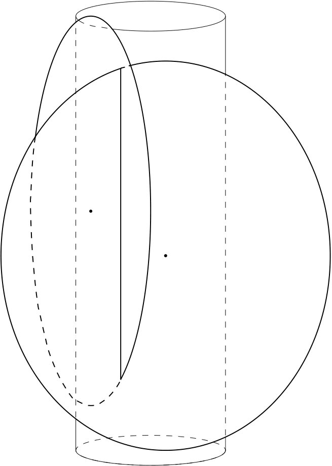 Figure 1
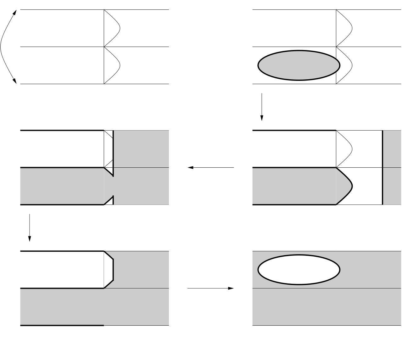 Figure 3
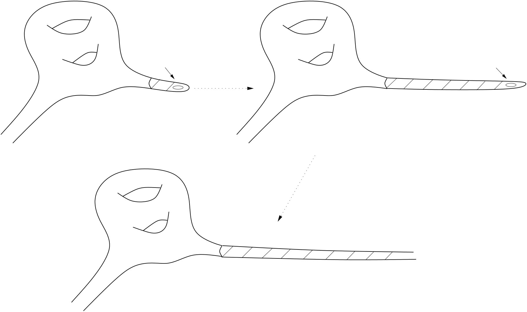 Figure 4
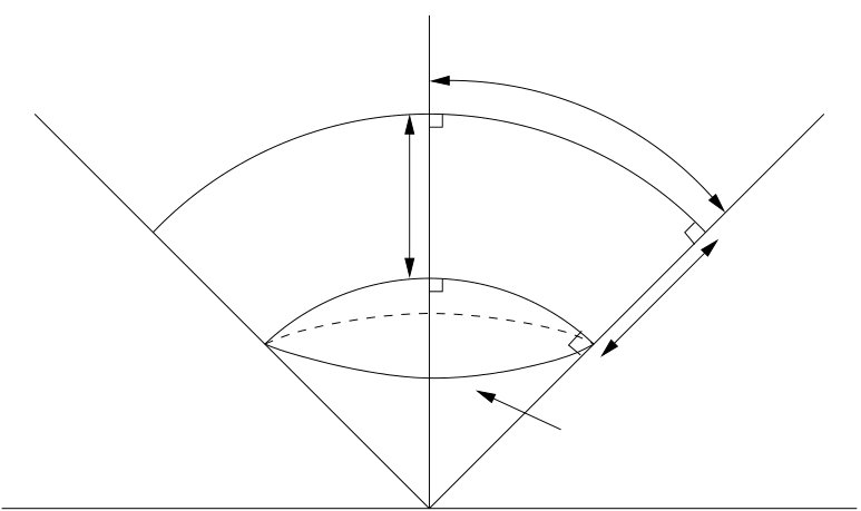 Figure 5