A Divide and Conquer Approach to Cooperative Distributed Model Predictive Control
He Kong, Stefano Longo, Gabriele Pannocchia, Efstathios Siampis, and, Lilantha Samaranayake

TL;DR
This paper introduces a novel divide and conquer cooperative distributed MPC framework that enables parallel local computations with guaranteed stability, reducing communication and synchronization requirements in linear systems.
Contribution
It proposes a state transformation-based approach allowing parallel local optimization without iterative cooperation, while maintaining stability guarantees.
Findings
Parallel local optimization without iterations is feasible.
Stability can be guaranteed with proper cost function design.
Numerical examples demonstrate the method's effectiveness.
Abstract
This paper is concerned with the design of cooperative distributed Model Predictive Control (MPC) for linear systems. Motivated by the special structure of the distributed models in some existing literature, we propose to apply a state transformation to the original system and global cost function. This has major implications on the closed-loop stability analysis and the mechanism of the resultant cooperative framework. It turns out that the proposed framework can be implemented without cooperative iterations being performed in the local optimizations, thus allowing one to compute the local inputs in parallel and independently from each other while requiring only partial plant-wide state information. The proposed framework can also be realized with cooperative iterations, thereby keeping the advantages of the technique in the former reference. Under certain conditions, closed-loop…
Click any figure to enlarge with its caption.
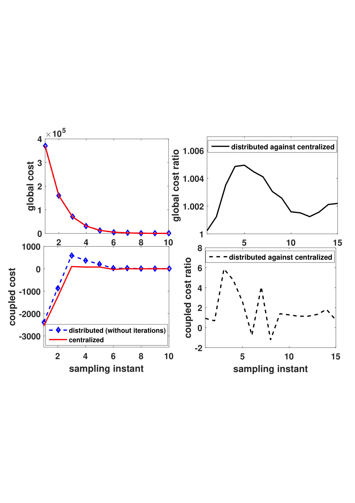 Figure 1
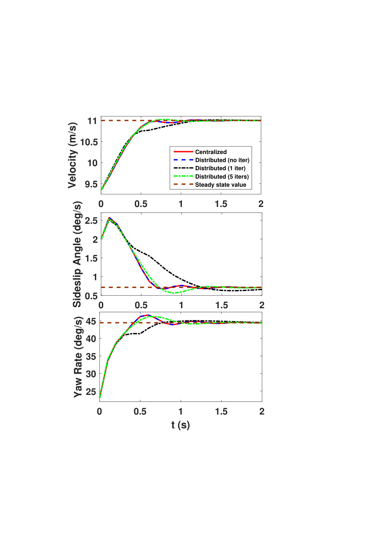 Figure 1
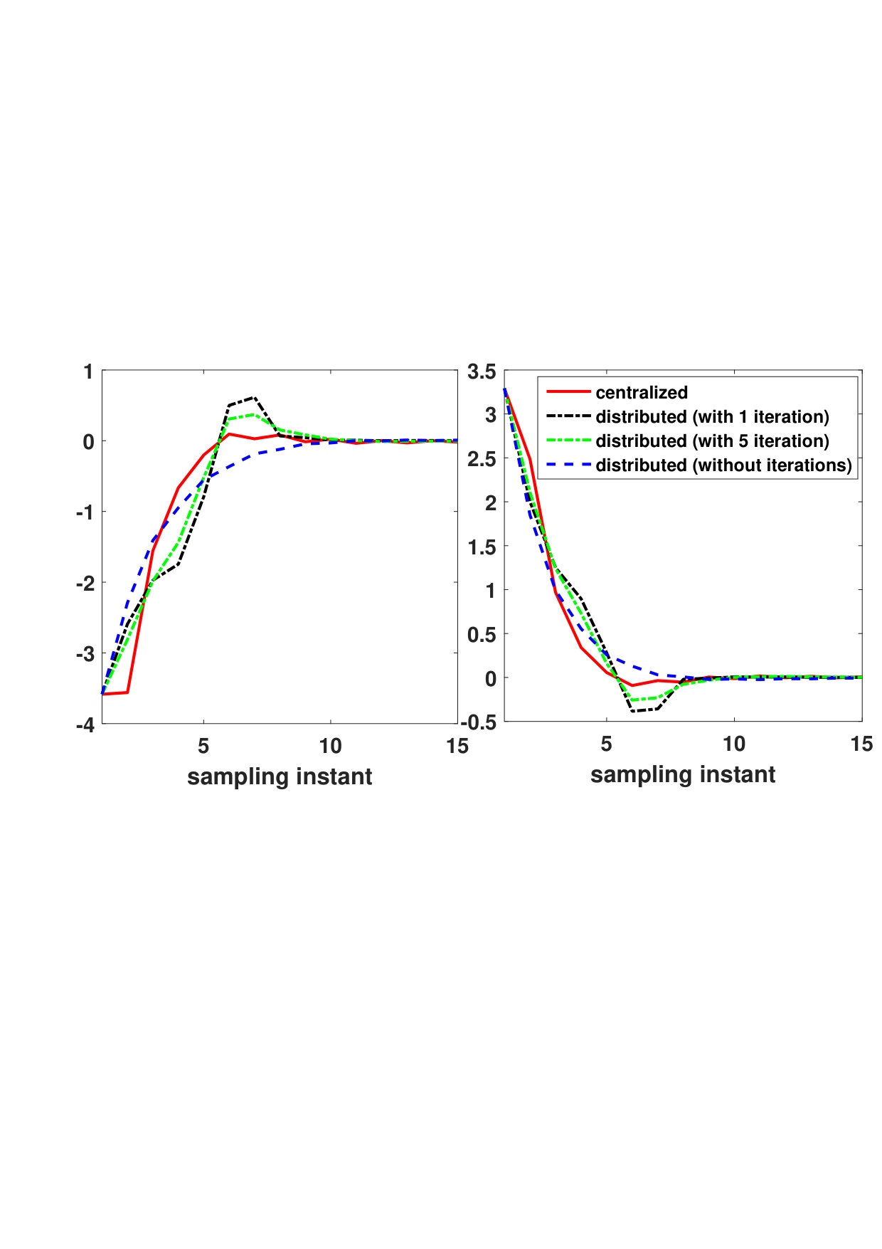 Figure 3
| Method | GC | GC loss | CC | CC loss |
|---|---|---|---|---|
| Centralized | 5.1029 | 0 | 178.3 | 0 |
| 5 iters | 5.1151 | |||
| 4 iters | 5.1218 | |||
| 3 iters | 5.1383 | |||
| 2 iters | 5.2018 | |||
| 1 iter | 5.5912 | |||
| no iters | 5.1671 |
| Method | Worse case | Average |
|---|---|---|
| Centralized | 0.0237s | 0.0085s |
| 5 iters | 0.0373s | 0.0257s |
| 1 iter | 0.0069s | 0.0055s |
| no iters | 0.0237s | 0.0094s |
Peer Reviews
No public reviews on file for this paper yet. If you reviewed it on a platform where reviews are public (OpenReview, ICLR, NeurIPS, ICML), you can paste yours below so the community can read it here.
Videos
No videos yet. Explain this paper in a talk, walkthrough, or lecture? Add one.
Taxonomy
TopicsAdvanced Control Systems Optimization · Fault Detection and Control Systems · Fuel Cells and Related Materials
A Divide and Conquer Approach to Cooperative Distributed Model
Predictive Control
He Kong, Stefano Longo, Gabriele Pannocchia, Efstathios Siampis, and Lilantha Samaranayake This work has been supported by the “Developing FUTURE Vehicles” project of the Engineering and Physical Sciences Research Council under the UK Low Carbon Vehicles Integrated Delivery Programme.He Kong was with the Advanced Vehicle Engineering Centre, Cranfield University, United Kingdom; he is now with the Australian Centre for Field Robotics, the University of Sydney, NSW, Australia, Email: [email protected]. Stefano Longo and Efstathios Siampis are with the Advanced Vehicle Engineering Centre, Cranfield University, College Road, Cranfield, United Kingdom. Email: s.longo, [email protected]. Gabriele Pannocchia is with the Department of Civil and Industrial Engineering, University of Pisa, Italy, Email: [email protected]. Lilantha Samaranayake is with Department of Electrical and Electronic Engineering, University of Peradeniya, Sri Lanka, Email: [email protected]
Abstract
This paper is concerned with the design of cooperative distributed Model Predictive Control (MPC) for linear systems. Motivated by the special structure of the distributed models in some existing literature, we propose to apply a state transformation to the original system and global cost function. This has major implications on the closed-loop stability analysis and the mechanism of the resultant cooperative framework. It turns out that the proposed framework can be implemented without cooperative iterations being performed in the local optimizations, thus allowing one to compute the local inputs in parallel and independently from each other while requiring only partial plant-wide state information. The proposed framework can also be realized with cooperative iterations, thereby keeping the advantages of the technique in the former reference. Under certain conditions, closed-loop stability for both implementation procedures can be guaranteed a priori by appropriate selections of the original local cost functions. The strengths and benefits of the proposed method are highlighted by means of two numerical examples.
Index Terms:
Model predictive control, Distributed control, Cooperative control, Constrained control
I Introduction
MPC relies on a dynamic model of the system of interest to predict its behavior into the future, and solves, at each sampling instant, a finite horizon optimization problem to determine an input sequence, while taking the system’s constraints into account [1]-[4]. This paper is inspired by the recent rigorous development in decentralized and distributed MPC [5]-[7]. Depending on the particular problem setups and associated solutions, existing distributed MPC methods could be classified in ways such as decentralized or distributed, cooperative or noncooperative [8]-[13]. Analysis and design of distributed MPC with network-induced effects has also received a considerable amount of attention [14]-[15]. For more detailed discussions on the properties of different distributed MPC methods, one can refer to [3, Chp. 6], [16]-[19].
This paper is concerned with the questions on whether and how the organizational system architecture can be utilized in the design of cooperative distributed MPC to facilitate the computation of local inputs and reduce the communication burden with stability guarantee. The importance of exploiting structural properties in synthesis and design of large-scale systems has been demonstrated in a number of works in control [20]-[21]. Another long-learned lesson is that understanding of architectural issues in controller design are frequently more important than optimizing within a given framework [22, Chp. 1, pp. 10-18]. A major motivation for developing the ideas in this paper is close in spirit to the above observations. To illustrate the concept, we adopt the problem setup in [23]. We advocate the utilization of a state transformation to the considered system and the original global cost function so that the intrinsic coupling effects in the original cooperative question are restructured and can be dealt with more effectively.
The proposed framework in this paper has the following advantages. Firstly, the proposed method can be implemented without cooperative iterations, if certain conditions hold (see in Propositions 1-2), with guarantee of global closed-loop stability. This allows one to compute local inputs in parallel and independently from each other, requiring only partial state information of other subsystems (besides the subsystem matrices information). This is in contrast to the standard cooperative MPC formulations [23] in which the computation of the local input requires plant-wide state information and inputs of other local systems, or at least of an *augmented local *system state [24]. Second, the proposed framework can also be realized with iterations as in [23], thereby keeping the merits of the standard cooperative method with iterations, e.g. convergence to the global centralized performance. Given the impact of the afore-mentioned state transformation on the original problem setup and the features of the proposed framework, we term the method the *Divide and Conquer (D&C) *approach.
The remainder of this paper is organized as follows. In Section II, preliminaries are given. Section III introduces the state transformation and analyzes its impact on the solution to the cooperative problem. Section IV contains stability analysis with state feedback for both the centralized and the distributed cases. Section V presents extensions and comparison discussions. Section VI contains two simulation case studies. Section VII concludes the paper. Notation: Most notation we use is standard. Matrices, whose dimensions are not stated, are assumed to be compatible for algebraic operations. denote the set of . denotes the Cartesian product of set for times. denotes a block diagonal matrix with and as its block entries. denotes .
II Preliminaries
This section recalls the problem setup from [23]. For simplicity, we assume that the overall plant consists of only two subsystems. The results will be extended to any finite number of subsystems in Section V. Assume for each subsystem is a collection of the linear discrete-time models
[TABLE]
where , , are constant system matrices; denotes the effects of input of subsystem on the states of subsystem . Denote By collecting the states of subsystem from (1), we can obtain:
[TABLE]
in which , A_{1}=diag(A_{11},A_{12}),\overline{B}_{11}=[B_{11},0],\overline{B}_{12}=[0,B_{12}],C_{1}=\left[\begin{array}[]{cc}C_{11}&C_{12}\end{array}\right]. The model of subsystem 2 can be obtained similarly. The plant-wide model then becomes
[TABLE]
where and . As remarked in [23], the model (3) is potentially non-minimal. Denote and the local input sequences for the two subsystems along the prediction horizon, respectively. We define the cost
[TABLE]
for subsystem 1 and for subsystem 2 similarly. The plant-wide cost function is , where and are positive real numbers. For simplicity, denote as the local and global cost functions, respectively. can be expressed in terms of the original centralized model (3) as:
[TABLE]
with , We assume that the local inputs must satisfy for , where both and are compact and convex sets that include the origin in their interior. For the case of decoupled input constraints, the contribution of either local input on cannot be affected by the other one in terms of feasibility. However, both and are functions of and because dynamics of both subsystems are dependent on either of the two local inputs. Thus, the computation of the optimal input sequence will still be dependent on , and viceversa. Therefore, for the local optimization problems of computing will be
[TABLE]
where, Depending on the method, other requirements have to be enforced in (6) for establishing closed-loop stability. For example, in [23], the prediction horizon has to be sufficiently long to zero the unstable system modes. In other cases [12, 24, 25], the usual terminal penalty and terminal region constraints are adopted. Closed-loop stability is typically proved by adopting the suboptimal strategy in [26]. For denote
[TABLE]
with being defined in (1)-(3). Obviously, we have where
[TABLE]
For , the following assumptions are made in [23] to establish stability: (A1) is stabilizable; (A2) ; (A3) and are detectable.
III The D&C Approach
III-A Dividing the system by a state transformation
From (3), one can notice that the model is of a special structure in the sense that each local input has only partial impact on both local systems. To be specific, from (1), for , one has , i.e., () can affect and ( and ). Given that is supposed to be stabilizable in Assumption A1, there exists such that is Schur stable, i.e., to stabilize the system with state feedback, for computing (), one only needs the information related to and ( and ). This motivates us to separate the modes of the subsystems into two categories that can only be affected by or , respectively. As such, we introduce a state transformation which renders a clearer inspection of the inherent structures of the original cooperative question (6). Denote
[TABLE]
One then has and with being defined in (2) and defined similarly. Denoting and substituting
[TABLE]
into the original plant model (3) gives us
[TABLE]
in which . Substituting into (11) gives with and being defined in (7). With (10), the plant state has been rearranged as such that
[TABLE]
where with and being defined in (8). It becomes evident that the original centralized model (3) has been divided into two parts that are only influenced by either or . However, important questions remain as how (10) impacts the cooperative cost function in (6). Besides, to apply the proposed method, one does not have to restructure the plant physically, since (10) is only to be utilized in the local optimization algorithms.
III-B Reformulating the cost by the state transformation
Substituting into (6) gives us:
[TABLE]
where, ,
[TABLE]
Structures of and depend on the original structures of and matrix . For , denote
[TABLE]
with
Remark 1
Given it follows that for
From (5), (9) and (14), after matrix manipulations, we have
[TABLE]
where, , and for , in which, with and as defined in (8). From Remark 1, we have when for . We arrive at an alternative formulation of the optimization problems (13). We believe this formulation is insightful because it shows clearly the impact of the individual local inputs on the global cost. To illustrate, the optimization problem for subsystem 1 now becomes
[TABLE]
where, with , , . From the structures of (11) and , we know that contains these parts that are only influenced by collects the coupling prediction dynamics between and embedded by and ; is only effected by and may be neglected when computing . Thus, it is that makes the computation of dependent on . This clearly raises the question about how this coupling term can be dealt with to facilitate the computation of local inputs and reduce communication burden.
IV Stability Analysis
IV-A The centralized case
The centralized MPC problem for (3) with the cost (5), after the transformation procedure in Section 3 is applied, is equavilent to the centralized MPC problem for (11) with the cost
[TABLE]
with , , and being defined in (16) and (5), respectively. To guarantee stability, the original terminal weigthing matrix has to be selected so that satisfies certain conditions. Based on Assumption A1, one can find such that
[TABLE]
is Schur stable. Given that contains the origin in its interior, for , there exists a (possibly small) polyhedral positively invariant set around the origin for so that for all Denote and
[TABLE]
One then has that is Schur stable. Moreover, becomes a local stablizing controller such that , for . Consider the following centralized MPC problem
[TABLE]
where, and is the input sequences for (11) along the prediction horizon. Denote the set of all for which there exists a feasible to (21). At each sampling instant, assume that is applied after the prediction horizon as a local controller in the set . Based on the terminal triple argument [3, Chp. 2], for system (11) in closed-loop with the solution to the centralized problem (21), stability can be obtained, if the original terminal weigthing is selected so that is the unique positive definite solution to the ARE
[TABLE]
i.e., . Note from (16), each of the four partitions of is block diagonal (BD), while as the solution to (22) does not necessarily have the same structure with . Thus, the question reduces to whether has specified structures as . This issue is closely related to the problem of structured Lyapunov functions and the requirement of having the same structure as in (16) would only be satisfied for systems with certain properties [27]. Without making such an assumption, an alternative sufficient condition for closed-loop stability is presented next. Denote
[TABLE]
Proposition 1
Select as in (19). Assume that is applied after the prediction horizon as a local controller in the set . If the terminal weigthing matrix in (4) have been selected such that satisfies the matrix inequality
[TABLE]
then the origin of the closed-loop system of (11) with the solution to (21), is exponentially stable in .
Proof:
Based on standard MPC stability arguments [3, pp.142-145], if is selected as in (19), and is applied after the prediction horizon as a local controller in the set , to establish stability, we only have to show that where . The above inequality holds if By deducting (22) from the above inequality on both sides, we obtain (24).
IV-B The distributed case
We proceed to establish the stability of the closed-loop system with distributed solutions. As in the previous subsection, for , we assume that is selected with a polyhedral positively invariant set around the origin for the system such that (19) is Schur stable and for all . Note that, and are generally not block diagonal (BD), i.e., in (15). However, from Remark 1, we still have when for with defined in (16). A closer look at the optimization problem (17) for computing reveals that as long as (defined in (12)) can be stabilized* by (similarly, stabilized *by ), the coupling term becomes an asymptotically vanishing weight that can be overlooked in the local optimization. Under such conditions, to compute , one only needs the information that is associated with , and there is no need of the information of and , e.g., there is no need to perform iterations in the local optimizations. In such cases, the resultant input sequence (and ) is a suboptimal solution to the original cooperative problem with cost function (5). In return, benefits of doing so are the large amount of communication burden reduction and the independency in computing the local inputs. In this case, the local optimization problems become
[TABLE]
where, is in the same form as in (17), with being defined in (16). Denote the set of all for which there exists a feasible to (25), for . At each sampling instant, assume that is applied after the prediction horizon.
Remark 2
Once we select the local costs as in subsection 2.1 (see in text before and after (5)) and follow the procedure in Section 3 to apply (10), the structures of the weightings in of (25) will be fixed. Especially, the terminal weighting is with a BD structure as specified in (16).
Therefore, the question reduces to whether the solution to the optimization problem (25), whose terminal costs have specified BD structures, can stabilize . In other words, if the ARE
[TABLE]
admits a BD positive definite solution having the same structure as in (16), closed-loop stability would follow based on the terminal triple argument [3, Chp. 2]. However, as noted in Remark 2, is with a BD structure. This problem is closely related to the question of diagonal stability and the requirement of having the same BD structure as in (16) would only be satisfied for systems with certain properties [28]-[29]. Alternatively, based on Proposition 1, we have the following result.
Proposition 2
Select as in (19). At each sampling instant, assume that is applied after the prediction horizon. If in (4) have been selected such that (24) holds, then in (16) satisfies the matrix inequality
[TABLE]
the origin of the closed-loop system of (11) with the solution to the problem (25) is exponentially stable in with and being computed independently.
Proof:
Given the structure of the reformulated system (11), closed-loop stability can be proved if we show that stabilizes . To illustrate, we show that if the original terminal weigthing matrix is selected such that (24) holds, then stabilizes . Note that if we ignore the terms and as in the optimization problem (25), the cost function becomes with , and Since the local terminal controller is applied beyond the prediction horizon, following standard MPC stability arguments [3, pp.142-145], we only have to show that satisfies This inequality holds if
[TABLE]
Given , in (20), in (5), (16), and the structure of in (23), the ARE (22) can be rewritten as
[TABLE]
Taking out the the first block diagonal components in the above expression gives us
[TABLE]
We can also obtain a more structured expression of (24):
[TABLE]
If the original terminal weighting matrices is selected such that (24) holds, the diagonal components of the the above inequality must hold, i.e., . Adding the above inequality and (29) from both sides gives (28). Therefore, stabilizes . A similar argument can be made so that stabilizes with and being ignored in the local optimization. The independency between the computation of and follows from the structure of the cost in (25).
To apply the proposed framework with stability guarantee, condition (24) has to be enforced as an additional requirement when selecting in (4), apart from the requirement that** .** Also, the satisfaction of condition (24) is a joint property of the considered system and the weightings and . Overall, Propositions 1-2 reveal that, within the proposed framework, local inputs can be computed independently while still guaranteeing plant-wide closed-loop stability, if condition (24) holds. Given the independency in computing the local inputs, there is a possibility to generalize the centralized tuning paradigms in [30]-[31] to the distributed case.
Remark 3
As remarked earlier, and in (5) are generally not BD. Given the arguments in the above stability analysis, one would be tempted to choose and/or to be BD, as long as they are compatible with the dimension of the state elements in (1). It is worthwhile emphazing that doing so is not sensible for the considered problem setup. The main reason for this is if both and are BD, by the BD structure of both the system (3) and the global cost (5), there will be no coupling terms at all in the local optimization (6), i.e., the distributed solution will always be the centralized solution, and there remains little motivation to consider such a scenario. Thus, to avoid this situation, for , either or has to be not BD.
IV-C Further remarks
Although the distributed policies without iterations resulting from (25) are a suboptimal solution to the original cooperative problem with cost function (5), they are actually optimal solutions to the following centralized problem
[TABLE]
where, , with being defined in (17) and defined similarly, and . Note that both the system dynamics and the cost functions in the above optimization problem are of a BD structure. Thus this optimization problem becomes separable for the local subsystems, rendering its solution same with that of (25). The only difference between the above optimization problem and the original cooperative question with cost function (5) is in the state weightings, i.e., the BD entries of state weightings in (5) (see the relationships in (14)) are taken out and placed in in (30). Denote Obviously, and become symmetric matrices with zero diagonal entries. Matrices with zero diagonal entries are also called hollow matrices. Generally speaking, and are indefinite, i.e., their eigenvalues might be positive, negative and zero. Therefore, the value of the coupled part in the global cost ( in (17)) may be positive or negative. We will illustrate this point in Section VI.
It should also be noted that the proposed D&C framework can be realized with iterations as in standard cooperative frameworks. If we adopt some warm start techniques and perform iterations in the local optimization as in standard cooperative frameworks, closed-loop stability of the D&C framework with iterations can be obtained if the terminal weighting in (4) have been selected such that (24) holds (this can be proved by following arguments in Proposition 1 and [23, Theorem 9], and we do not present further details here). An important observation to be made here is that closed-loop stability for the system (11) with the centralized solution, the distributed solution without or with iterations, respectively, can be guaranteed simultaneously by selecting the terminal weigthing matrix in (4) so that (24) holds, i.e., one can change the implementation method during operation without affecting the closed-loop stability.
We next present a sufficient condition for (24) to hold. A matrix A\in\mathbf{R}^{n\times n}\is diagonally dominant (DD) if , for [32, pp. 392].
Corollary 1
Denote as the solution to the ARE (22). If the terminal weigthing matrix in (4) have been selected such that is DD with nonnegative diagonal entries, then condition (24) holds.
Proof:
From [33, pp. 15], a DD and symmetric matrix with nonnegative diagonal entries is positive semidefinite. Given as the solution to the ARE (22), if the original terminal weigthing matrix in (4) is selected so that is DD with nonnegative diagonal entries, the former matrix is positive semidefinite. Therefore, condition (24) holds.
V Some Generalizations and Discussions
With subsystems, the plant-wide system becomes:
[TABLE]
where, for with and in similar structures with and in (2) and (3), respectively. Denote . The global cost is , where takes the form of in subsection 2.1. To compute , each local system solves
[TABLE]
where is with a similar structure to that of in (6). We propose the transformation , where
[TABLE]
and, with \widetilde{n}_{i}=\sum\limits_{j\in\mathscr{I}_{1:M}}n_{ij}\and is a BD matrix with its -th block entry as an identity matrix of dimension and other entries as zeros, for for and , is a block partitioned matrix with its entry as an identity matrix of dimension and other block entries as zeros; for and , is a block partitioned matrix with its entry as an identity matrix of dimension and other block entries as zeros. Moreover, it can be verified that , i.e., The impact of the transformation on the system (31) and the cost functions (32) can be conducted as in Section III. Stability analysis can also be established as in Section IV.
Moreover, the results in Sections III-IV for the case with state feedback can be extended to the case with output feedback by embellishing the ideas in Sections III-IV with decentralized estimation (based on Assumption A3). Then the problem at hand becomes robust stability analysis in the presence of bounded (decaying) disturbances, and can be dealt with by applying robust MPC techniques such as tube-based MPC or by exploiting the inherent robustness properties of suboptimal MPC [34]. We do not present detailed discussions here due to limited space.
A summary of the comparisons between the proposed method and the technique in [23] is presented in the Table I. It can be concluded that the proposed method, without iterations, requires lower information and communication overhead than the technique in [23], while still enjoying the advantages of the stability properties, as well as convergence to the global centralized performance, when implemented with iterations.
It will be hard to make a comprehensive comparison between the proposed method and many other existing techniques. Despite the potential advantages of the proposed method, it has been noted already that the adopted model might be non-minimal. We also remark that the assessment of a specific method should not only be based on the method itself but also the particular targeted application. Moreover, only the case of decoupled inputs is considered in this paper. Whether and how the proposed framework can deal with coupled input constraints remains as an interesting future topic. Another topic of interest is to extend the method to linear programming (LP), for which some preliminary results have been presented in [35].
VI Illustrative Examples
VI-A An academic example with three subsystems
The first example is presented to show the controller design procedure of the proposed framework. The considered system is composed of three subsystems. The local systems in (31) are defined by , , , in which
[TABLE]
Since we have for the state transformation matrix is T=\left[\begin{array}[]{ccc}T_{{}_{1,1}}&T_{{}_{1,2}}&T_{{}_{1,3}}\\ T_{{}_{1,2}}^{\mathrm{T}}&T_{{}_{2,2}}&T_{{}_{2,3}}\\ T_{{}_{1,3}}^{\mathrm{T}}&T_{{}_{2,3}}^{\mathrm{T}}&T_{{}_{3,3}}\end{array}\right]\in\mathbf{R}^{18\times 18}, where, with is generated from the structure of (33). The three local inputs are assumed to satisfy for The original local stage cost of each subsystem is defined by , where, Q_{1}=\left[\begin{array}[]{ccc}10I&2I&3E\\ 2I&15I&3E\\ 3E&3E&20I\end{array}\right], with standing for square matrices having all its entries as 1, and is to be designed. The relative weights of the local cost functions are , We follow the procedure in Section 3 and apply the state transformation to the original system and the global cost function. For each open-loop unstable virtual subsystem, a local stabilizing LQR controller is designed with the following weights It can be verified that the unit ball of dimensions around the origin becomes a positive invariant set for the three virtual subsystems in closed-loop with their local LQR controllers, respectively. Therefore, this set has been enforced as a terminal constraint in the local optimization problems (25). The terminal costs in (4) are selected so that the condition (24) and the requirement that hold simultaneously. The prediction horizon is chosen to be .
(i) We firstly compared the distributed solution without iterations and the centralized solution. The initial states of the original subsystems are taken to be x_{1}=\left[\begin{array}[]{cccccc}-10&-4&9&7&8&5\end{array}\right]^{\mathrm{T}}, x_{2}=\left[\begin{array}[]{cccccc}-8&-5&7&3&3&6\end{array}\right]^{\mathrm{T}}, x_{3}=\left[\begin{array}[]{cccccc}-5&-6&8&-9&8&3\end{array}\right]^{\mathrm{T}}. At each sampling instant, we compute the value of the global cost (GC) with the distributed solutions without iterations and the centralized solution, respectively. Note that when computing the distributed solutions without iterations, the coupled parts in the global cost (as in (25) for the case with 2 subsystems) are ignored. To better compare the distributed solution without iterations against the centralized solution, we will also compare the cost value of the coupled parts with either solution, respectively. To make a fair comparison, the state information for both centralized and distributed optimization problems at each sampling instant is updated by the distributed solution, i.e., the states are enforced to be the same for both optimization problems and it is the ways the two solutions being computed make the difference in the value of the GC and the coupled parts. The simulation results are illustrated in Figure 1. It can be seen from Figure 1 that the distributed solution always renders slightly worse performance than the centralized solution for the GC. Nonetheless, the global performance loss is very moderate and remains within . Regarding the coupled cost (CC), it can be observed that its value can change sign due to the discussions made after (30). The value of the coupled cost with the distributed solution is always larger than that with the centralized solution. This is not unexpected, since the coupled part has been included in the centralized optimization but not in the distributed optimizations.
Note that in the above simulation, the distributed solutions are computed via optimization problems (25), i.e., the coupled parts and in (17) have not been considered. However, the values of the CC have been added when calculating the value of the GC with distributed solutions. To understand better the performance loss of the distributed solution without iterations, we draw 1000 sets of initial states whose entries are random variables between The average global performance loss from these 1000 random initial conditions is obtained to be within and the worse global performance loss is less than Note that compared to the centralized solution, the local distributed solution without iterations only needs (for this particular example) of the global state information, and does not require the information of other local inputs.
(ii) We next compare the distributed solution without iteration, standard cooperative solution (with iterations) and the centralized solution. For this purpose, we take the initial conditions of the original subsystems to be x_{1}=\left[\begin{array}[]{cccccc}10&10&8&6&-6&6\end{array}\right]^{\mathrm{T}}, x_{2}=\left[\begin{array}[]{cccccc}10&2&3&5&3&6\end{array}\right]^{\mathrm{T}}, x_{3}=\left[\begin{array}[]{cccccc}6&-4&4&2&2&3\end{array}\right]^{\mathrm{T}}. For the first three sampling instants we use the distributed solution without iterations to initialize the optimization procedure. For the three strategies, we use the state information at the fourth sampling instant as the initial conditions, i.e., the initial condition is chosen to be the same for three different methods. Also, the shifted input sequences of the distributed solution without iterations are used as warm starts in obtaining the standard cooperative distributed MPC solution with iterations.
We compare the value of the GC and CC associated with distributed solution (without and with iterations) against the centralized solution. The results are summarized in the Table 2. From Table 2, it can be seen that the value of GC with the distributed solution without iterations is smaller than that of standard cooperative distributed solution with 1 iteration. Moreover, the strategy with iterations outperforms the case without iterations in that the value of the CC with iterations is smaller. When more iterations are conducted, the performance of the solution with iterations improves and becomes better than the solution without iterations. Besides, as more iterations are performed, the performance of the distributed strategy improves, and with just 5 iterations, its global performance loss reduces to less than . One can also verify that when a large number of iterations is conducted, the standard cooperative distributed solution converges to the centralized solution.
(iii) Finally, we compare the closed-loop trajectories of the system with different control strategies, respectively, using the initial conditions of the second simulation (ii). For the first sampling instant, we use distributed solution without iterations to initialize the optimization procedure. From the second sampling instant, the state information at each sampling instant is updated by different strategies, respectively. In Figure 2, we show the closed-loop trajectories of with different control strategies. It can be seen that the centralized solution offers the best performance among all the strategies; the standard cooperative distributed solution with 5 iterations can render a slightly quicker response than the solution without iterations and with 1 iteration. Also, the response of the solution with 1 iteration is slightly slower than that of the solution without iterations.
We have run this set of simulation for 200 sampling instants and solved the QPs using quadprog in Matlab on a desktop computer with the processor Intel Xeon Processor E5-2650 v2 (processor base frequency 2.6 Ghz). A summary comparison of the computation time of different strategies is shown in Table 3. Note that we choose the worse case scenario among all the local inputs for calculating the execution time for the solutions with iterations at each sampling instant. To be more specific, for solutions without iterations and with 1 iterations, if the execution time at a certain sampling instant, for the three local inputs is , , , respectively, we then choose the largest one of the three as the computation time for the current sampling instant. For the standard cooperative distributed solution with 5 iterations, the execution time at a certain iteration within a certain sampling interval, for the three local inputs is with , , we choose the largest value of , given , as the computation time for the current sampling instant. A similar procedure is carried out at each sampling instant, the worse case and the averge computation time in Table 3 is then calculated from the record for the 200 simulations. From Figure 2 and Table 3, we can see that the standard cooperative distributed solution with iterations generally takes more time to compute with potentially improved performance. It should also be noted that the worse case computation time for the centralized solution is not significantly different from that of the solutions without iterations or with 5 iterations. This is not very surprising given the moderate complexity of the example. Also, as it has been remarked in [23], a major argument to develop distributed methods, as opposed to a centralized solution, is often not computational, but organizational, i.e., in the latter case, all subsystems rely on a central decision maker to coordinate and maintain plant-wide actions, leading to organizational inefficiency, implementation and maintenance difficulties.
Based on all the previous simulations, we conclude that the distributed solution without and with iterations have their respective advantages. We suggest that one should adopt a combination of these two implementation methods. For example, one could use the solution without iterations to initialize the distributed algorithm; and perform iterations for certain steps in the transient process to potentially reduce the coupled costs as well as improve the global performance; as the states approach the origin, one could switch back to the solution without iterations. Note that as long as the local weights are selected so that the condition (24) holds, a change of the implementation method during operation would not affect closed-loop stability.
VI-B Cooperative distributed control of a four-wheel vehicle
To see the applicability of the proposed method to a practical problem, we apply the technique to a four wheel drive (4WD) vehicle dynamics problem with four independent wheel motors [36]. Whilst the application of MPC to vehicle dynamics problems is not new, the main motivation of examining the cooperative distributed MPC technique here is to potentially improve the vehicle stability by distributedly controlling the torques to four independent wheel motors while considering their respective impact on the whole vehicle. Note that the vehicle and tyre models used in this example were originally proposed in [37] and are very similar to those in [36]. The interested reader can refer to [36]-[37] for more technical details such as the description of the equations of motion, tyre models, etc. The vehicle under consideration in this example is a small sports car with parameters reported in [36]. In order to control four wheel motors in a distributed way, we partition the centralized discrete-time model into 4 subsystems by assuming that the information of the vehicle velocity , the sideslip angle , the yaw rate , and the four motors’ respective torque information is available at each local subsystem via the vehicle bus communication network. We also assume that a constant steering input of is applied on both the front wheels. To apply the proposed cooperative distributed MPC technique, we linearize the vehicle dynamics model around the steady state (SS) cornering condition and derive a centralized linear discrete-time model with sampling time 0.1 s. The prediction horizon is selected to be . The wheel torque is required to stay within the specified motor torque limits of .
We compare four different strategies, i.e., centralized, distributed (no iterations), distributed (1 iterations), and distributed (5 iterations), against each other with the original nonlinear vehicle dynamics model in closed-loop. For the first step, with a given state information, we use the distributed solution without iterations to initialize the whole procedure. Starting from the second sampling instant, the closed-loop state information is updated by the four different methods, respectively. The responses of vehicle velocity, sideslip angle and yaw rate are shown in Figure 3. It can be seen from Figure 3 that the four different methods all offer fairly quick responses. More closely, the distributed solution with 1 iteration renders comparable but slightly worse performance than that of centralized, distributed without iterations, and distributed with 5 iterations. We notice similar patterns in the wheel speed response and due to limited space, these results are not shown here. Note that in Figure 3, the vehicle dynamics response with the centralized method and the distributed solution without iterations are close to, but not the same with, each other.
VII Conclusions
This paper has presented a Divide and Conquer approach to the design of cooperative distributed MPC. By recognizing the inherent structure of the problem setup in distributed MPC, we propose to apply a state transformation to the original cooperative problem so that the coupling effects in the original problem setup can be dealt with more effectively. Implications of the state transformation and sufficient conditions for closed-loop stability are thoroughly discussed. For the case without iterations, the proposed method allows one to compute the local inputs independently from each other with partial plant-wide state information, thereby potentially saving a large amount of communication overhead. The framework can also be implemented with iterations, thereby keeping the merits of the standard cooperative techniques with iterations. Starting from the case of 2 systems, we have also presented the generalization to systems, and two numerical application examples which show the benefits of the proposed framework.
Acknowledgment
The authors thank Dr. Efstathios Velenis at Cranfield University, for kindly providing the original code in [37] which we used to complete the simulation work in the second example.
The reference list from the paper itself. Each links out to its DOI / PubMed record.
- 1[1] D. Q. Mayne, J. B. Rawlings, C. V. Rao, and P. O. M. Scokaert, Constrained model predictive control: Stability and optimality, Automatica, Vol. 36, Issue 6, pp. 789-814, 2000.
- 2[2] J. M. Maciejowski, Predictive control with constraints, Prentice Hall, Inc., New Jersey, 2001.
- 3[3] J. B. Rawlings and D. Q. Mayne, Model predictive control: theory and design, Nob Hill Publishing, LLC, Madison, 2009.
- 4[4] D. Q. Mayne, Model predictive control: recent developments and future promise, Automatica , Vol. 50, No. 12, pp. 2967–2986, 2014.
- 5[5] G. Pannocchia, S. J. Wright, and J. B. Rawlings, Efficient cooperative distributed MPC using partial enumeration, Proc. of ADCHEM , Vol. 7, No. 1, pp. 607-612, 2009.
- 6[6] J. B. Rawlings and B. T. Stewart, Coordinating multiple optimization-based controllers: new opportunities and challenges, Journal of Process Control , Vol. 18, No. 9, pp. 839–845, 2008.
- 7[7] K. V. Ling, J. M. Maciejowski, A. Richards, and B. F. Wu, Multiplexed model predictive control, Automatica , Vol. 48, No. 2, pp. 396–401, 2012.
- 8[8] T. Keviczky, F. Borrelli, and G. J. Balas, Decentralized receding horizon control for large scale dynamically decoupled systems, Automatica , Vol. 42, No. 12, pp. 2105–2115, 2006.