Distributed synaptic weights in a LIF neural network and learning rules
Beno\^it Perthame (MAMBA, LJLL), Delphine Salort (LCQB), Gilles, Wainrib (DI-ENS)

TL;DR
This paper investigates how the distribution of synaptic weights in a large-scale LIF neural network affects its activity and learning capabilities, highlighting the role of noise in signal memorization.
Contribution
It analyzes the impact of synaptic weight distributions on network behavior and introduces simple learning rules that shape these distributions.
Findings
Synaptic weight distribution influences network discrimination capacity.
Learning rules can generate specific synaptic weight distributions.
Noise acts as a selection mechanism and aids in memorization.
Abstract
Leaky integrate-and-fire (LIF) models are mean-field limits, with a large number of neurons, used to describe neural networks. We consider inhomogeneous networks structured by a connec-tivity parameter (strengths of the synaptic weights) with the effect of processing the input current with different intensities. We first study the properties of the network activity depending on the distribution of synaptic weights and in particular its discrimination capacity. Then, we consider simple learning rules and determine the synaptic weight distribution it generates. We outline the role of noise as a selection principle and the capacity to memorized a learned signal.
Click any figure to enlarge with its caption.
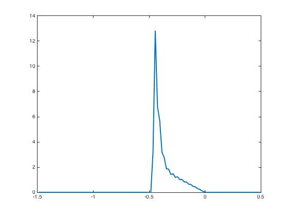 Figure 1
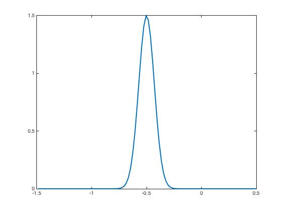 Figure 2
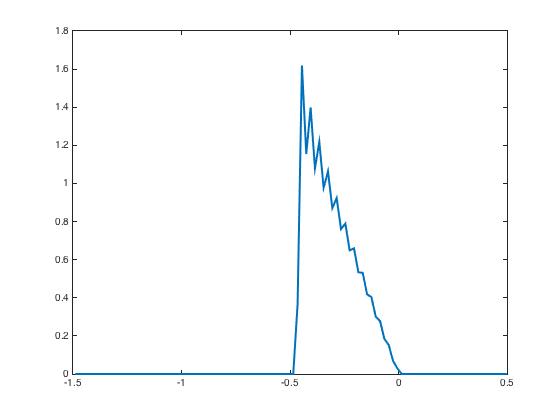 Figure 3
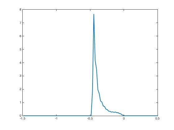 Figure 4
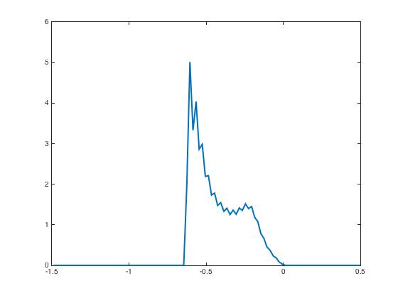 Figure 5
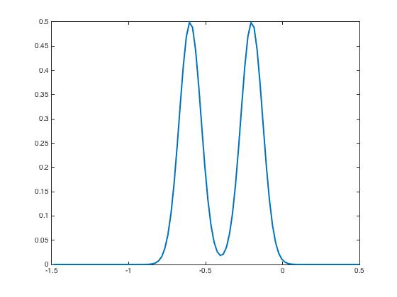 Figure 6
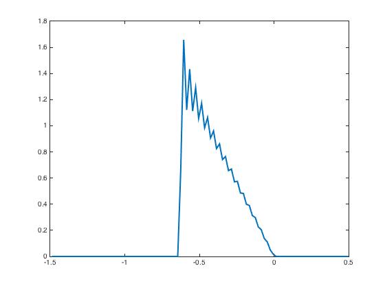 Figure 7
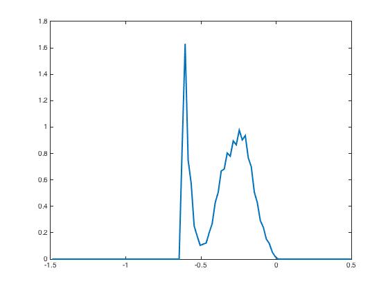 Figure 8
Peer Reviews
No public reviews on file for this paper yet. If you reviewed it on a platform where reviews are public (OpenReview, ICLR, NeurIPS, ICML), you can paste yours below so the community can read it here.
Videos
No videos yet. Explain this paper in a talk, walkthrough, or lecture? Add one.
Distributed synaptic weights in a LIF neural network
and learning rules
Benoît Perthame Sorbonne Universités, UPMC Univ Paris 06, CNRS UMR 7598, Laboratoire Jacques-Louis Lions, Inria Équipe MAMBA, 4, place Jussieu 75005, Paris, France, Email: [email protected]
Delphine Salort Sorbonne Universités, UPMC Univ Paris 06, CNRS UMR 7238 , Laboratoire de Biologie Computationnelle et quantitative, 4, place Jussieu 75005, Paris, France, Email: [email protected]
Gilles Wainrib Ecole Normale Superieure France, Département d’Informatique, équipe DATA, Paris, France, Email: [email protected]
Abstract
Leaky integrate-and-fire (LIF) models are mean-field limits, with a large number of neurons, used to describe neural networks. We consider inhomogeneous networks structured by a connectivity parameter (strengths of the synaptic weights) with the effect of processing the input current with different intensities.
We first study the properties of the network activity depending on the distribution of synaptic weights and in particular its discrimination capacity. Then, we consider simple learning rules and determine the synaptic weight distribution it generates. We outline the role of noise as a selection principle and the capacity to memorized a learned signal.
Key words: Neural networks; Learning rules; Fokker-Planck equation; Integrate and Fire;
Mathematics Subject Classification (2010): 35Q84; 68T05; 82C32; 92B20;
1 Introduction
Learning and memory are essential cognitive functions which are supported by the subtle mechanisms of synaptic plasticity [26]. Since the seminal work of Hebb [22], one of the key challenges in theoretical neuroscience and artificial intelligence is to understand the consequences of various learning rules on the organization of neural networks and on the way they process and memorize information.
Despite several theoretical works on this topic [21, 15, 20, 19, 18] it remains difficult to investigate learning processes using macroscopic models with infinite number of neurons because these usually assume a form of homogeneity, either under uniform synaptic weights assumptions leading to McKean-Vlasov limits [13, 2, 16, 17, 3] or under random connectivity models leading to dynamical spin-glass limits [28, 1]. In contrast, when studying synaptic plasticity and learning, one needs to describe all the connections between each pair of neurons, hence breaking the homogeneity usually necessary to derive such macroscopic limits.
In this article, we propose a way to circumvent this difficulty by introducing a mathematical model describing a macroscopic population of leaky integrate-and-fire neurons (LIF in short), which are interacting through a mean-field variable and where learning rules are governed by the mean activity of the network. More precisely, in contrast with previous works on such questions, we consider a model where neuronal subpopulations interact with the mean-field through a heterogeneous distribution of synaptic weights values: in other words, each subpopulation sees the mean-field through a different lens. Instead of considering activity-dependent changes in the pairwise synaptic weights between neurons, we consider that each subpopulation receives a weighed version of the overall network activity, and that the associated weights can be dynamically modified according to a specific rule. Based on this heterogeneous model, we are therefore able to integrate a learning rule term in the equation, for the first time in the class of macroscopic LIF equations. One particular instance of such learning rule corresponds to the idea of Hebbian learning, in the sense that the connection between a given subpopulation and the mean-field is strengthen if both have a correlated activity and is weakened otherwise.
The introduction of this mathematical framework supports the investigation of several questions inspired by the seminal work of Hopfield [23], which are answered, at least partially, in this article:
For a given pattern of steady-state neural activity, can we always find a heterogeneous synaptic weight distribution that generates such activity? 2. 2.
What is the equilibrium synaptic weight distribution according to the learning rule and to the external signal? 3. 3.
Is the system able to remember which external signal was presented during the learning phase?
We present in Section 2 the different mathematical models that we consider in order to study the effect of a mean field learning rule on coupled neural networks governed by Noisy LIF models structured by a connectivity parameter. In Section 3, we introduce some material about the possible stationary solutions of these models without learning rule, in particular we study existence and uniqueness. This material will be use throughout the paper. Next, we focus our study on qualitative properties on the input-output map and on the learning rules. In Section 4, we prove that our model can produce a large class of output signals by an appropriate choice of the distribution of connectivity. In Section 5, we show the ability of our model to differentiate different inputs via a discrimination property: we prove that we cannot obtain the same output signal considering two different input signals and, given two different inputs, we give an estimate of the difference between the two possible output signals associated to two different inputs. The last sections are devoted to the study with the learning rule. In Section 6, we address the full system with learning and we describe possible equilibrium connectivity distributions and prove non-uniqueness. We propose in Section 7 a selection principle by adding noise in the learning stage. In Section 8, we describe the ability of such system to memorize learned signals by discriminating easily new incoming inputs after learning.
2 Mathematical models of a mean field learning rule
It is standard to describe homogeneous neural networks by LIF models. In order to study the impact of heterogeneity and of mean field learning rules, we introduce a mathematical model for coupled neural networks. To this end, we firstly explain the equations which describe the activity of a macroscopic population of LIF neural networks when they interact through they mean activity. Secondly, we present how mean field learning rules may be included in these equations.
2.1 Structured Noisy LIF model
We consider a heterogeneous population of homogeneous neural networks structured by their synaptic weights , negative sign stands for inhibitory neurons and positive sign for excitatory neurons. We have chosen to use a signed parameter , instead of a system of two equations for excitatory and inhibitory neurones, because this leads to a simpler formalism and avoids boundary conditions in .
We assume that each homogeneous subpopulation, with synaptic weight , is governed by the classical mean field noisy integrate and fire equation, widely used for large neural networks [7, 6, 5]. Moreover, we assume that the subpopulations interact via the total firing rate defined as the mean activity for all the subpopulations. Setting the value of the action potential, the values of the firing and reset potentials, we consider the classical equation
[TABLE]
with the boundary and initial conditions
[TABLE]
The solution defines the probability to find a neuron at potential with a synaptic weight , the coefficient represents the synaptic noise which we assume to be constant and is the input signal which strength is possibly modulated by the synaptic weights. The subnetwork activity and total activity are defined as
[TABLE]
The function represents the response of the network to the total activity. We use either , or the following class with saturation
[TABLE]
We recall some mathematical properties of distributional solutions of Equation (1)–(3) which were studied in [8, 10, 11]. There, some existence, uniqueness and long time behaviour results are established for distributional solutions. For excitatory networks, solutions can blow-up in finite time, as discovered in [8], when . The saturation assumption (4) prevents blow-up, a phenomena which also appears if one uses the activity dependent noise [11]), or if a refractory state is included [9]. In the inhibitory case, blow-up never occurs when noise is independent of the activity [10, 11] and solutions are globally bounded. This holds even for and assumption (4) is not fundamental in the inhibitory case. Then, the main open problem which remains is to prove the long time convergence; only small perturbations of the linear case are treated so far.
The initial data is a probability density and a basic property of the above LIF model is that
[TABLE]
We finally define the probability density of neural subnetworks with synaptic weight by
[TABLE]
Let us mention that, so far, the function is independent of time because in Equation (1), the distribution of synaptic weights is fixed. Moreover, with this distribution , an input signal is stored as a normalized output signal which we define thanks to the network activity as
[TABLE]
The normalization is due to the size of the network normalized by which induces a limitation of possible outputs.
Let us now include some learning rules that may modify this distribution.
2.2 Models with mean field learning rules.
Next, we introduce some learning rules in order to modulate the distribution of synaptic weights and allow the network to recognize some given input signals by choosing an appropriate heterogeneous synaptic weight distribution adapted to the signal . To this end, we have chosen learning rules inspired from the seminal Hebbian rule which essentially consists in assuming that the strength of weights between two neurons and increases when the two neurons have high activity simultaneously. For neurons in interactions, the classical Hebbian rule relates the weights to the activity of the neuron
[TABLE]
In our context, we assume that the subnetworks interact only via the total firing rate , with synaptic weights described with a single parameter , not a matrix. Hence, we cannot generalize directly the Hebbian learning rule and we give the following interpretation. All the subnetworks parametrized by may modulate their intrinsic synaptic weight with respect to a function which depends on the intrinsic activity of the network parametrized by and of the total activity of the network . Then, the proposed generalization of the Hebbian rule consists in choosing
[TABLE]
where represents the learning strength of the subnetwork with synaptic weight .
Adding the above choice of learning rule, we obtain the following equation
[TABLE]
with the boundary and initial conditions
[TABLE]
Here, stands for a time scale which takes into account that learning is slower than the normal activity of the network, and \Phi=\Phi\big{(}N(w,t),\bar{N}(t)\big{)} represents the learning rule. Notice that a desirable property is that the flus is inward which occurs for instance when is bounded or sub-linear at infinity. Several direct extensions of the Hebbian rule are possible for example
[TABLE]
or inspired from STDP rule (spike timing dependent plasticity, see [21] for instance), where post- and pre-synaptic spike times are compared, we may choose
[TABLE]
Here for and for .
3 Stationary solution of the nonlinear problem without learning rule
Throughout this paper we use some material about the possible stationary solutions of Equations (1)–(3) submitted to a given input signal . These stationary states are defined through the equation
[TABLE]
with the boundary conditions
[TABLE]
We recall that the nonlinearity is driven by the network total activity defined as
[TABLE]
and that we assume a normalization (5) which is written
[TABLE]
Our first result is the
Theorem 3.1** (Existence of stationary states)**
We assume (4), give the input signal and the synaptic weight distribution normalized to such that there exists with
[TABLE]
*Then, there is at least one solution of (10)–(13).
In the case of inhibitory network, that is , for all , the solution is unique.*
Let us mention that for a single , semi-explicit formula are available, see [8] for instance, and the stationary states are not necessarily unique in the excitatory case.
Proof. Our approach is to solve the nonlinear problem using a fixed point argument on the value . Being given , and , we consider the linear problem where is a parameter (we do not repeat the boundary conditions)
[TABLE]
Let defined by
[TABLE]
Then, we obtain a solution of (10)–(12) if and only if is a fixed point of the application , that is
[TABLE]
To prove the existence of such a fixed point, we need a careful analysis of the mapping , which we perform in the next subsection, adding many properties that will be used later on. The conclusion of the proof is given afterwards.
3.1 Main properties of in (15)
Being given , the linear stationary state Equation (15), because it is solved by , is a standard equation and solutions form a one dimensional vector space (the eigenspace for the eigenvalue [math]) according to the Krein-Rutman theorem [14]. Uniqueness is enforced thanks to the normalization as a probability.
Integrating Equation (15), we obtain that a solution satisfies
[TABLE]
with to be found such that . Hence, the solution is explicitly given by
[TABLE]
with
[TABLE]
which is also written under the more convenient form
[TABLE]
Because of the boundary condition , an immediate consequence of (17) is the relation
[TABLE]
Throughout the paper, we use properties of the function which we state in the following lemma.
Lemma 3.2
*Given and , the unique solution of Equation (15), defined by (18)-(19), satisfies the following estimates. There is a constant such that *
[TABLE]
[TABLE]
[TABLE]
[TABLE]
Moreover, when , the following estimates holds
[TABLE]
[TABLE]
Proof of Lemma 3.2. We first prove inequality (21). We set where . As
[TABLE]
we obtain, with formula (19), that there exists a constant such that
[TABLE]
Therefore, we conclude the upper bound with
[TABLE]
For the lower bound, we set
[TABLE]
and conclude that
[TABLE]
Inserting this lower bound in formula (19), we deduce that there exists a constant such that
[TABLE]
We deduce that there exists a constant such that
[TABLE]
which ends the proof of estimate (21).
Next, we prove the inequality (22). We have, for all ,
[TABLE]
Because for , we have almost everywhere in and
[TABLE]
To prove the estimate (23), we differentiating the explicit formula of with respect to . We obtain that
[TABLE]
which directly gives (23).
To prove (24), we observe that, when ,
[TABLE]
Next, when , we have
[TABLE]
Therefore, we obtain estimate (25) because for , we have
[TABLE]
Finally, the inequality (26) follows from
[TABLE]
The proof of Lemma 3.2 is complete.
3.2 Conclusion of the proof of Theorem 3.1
We come back to the fixed point equation (16). With the above notations, it is restated, using the quantity defined by (19), as a fixed point of the function
[TABLE]
We have .
In the inhibitory case, when supp, we have thanks to (23), and thus there is a unique fixed point.
When excitatory weights are considered, as
[TABLE]
we have to impose an additional assumption on to control . For this purpose, using estimate (21), thanks to the assumption (14), we know that remains bounded and hence, there is at least one fixed point by continuity.
4 Output signals induced from a synaptic weight distribution
As a first property of the network properties, we aim at identifying which possible steady states output activities or signal can be generated by the network by varying the synaptic weight distribution .
We prove that any nonnegative normalized output signal , with fast decay at , can be, up to a multiplicative constant, reproduced by a stationary state of Equation (10) for a well chosen synaptic weight distribution .
Theorem 4.1** (Relation output signal to synaptic weights)**
*We assume (4) and give the input signal and the output signal normalized with and satisfyning with . Then, we can find a synaptic weight distribution normalized to , such that (7) holds true for a solution of (10)–(13).
In the case of inhibitory signal, that means , for all , the synaptic weight distribution and are unique.
Proof. Consider an output normalized signal . Using the notations of section 3, the relations (7) are reduced to building a distribution normalized to , such that the following relations hold
[TABLE]
and the fixed point condition (16) is automatically satisfied thanks to the normalization of .
In other words, we look for such that
[TABLE]
Let us mention that because of estimate (22) and the integrability condition on .
These conditions are reduced to achieve the value by the mapping defined by
[TABLE]
We have obviously . Moreover, using the last estimate of (22), we obtain that
[TABLE]
and so which implies existence of the activity satisfying the desired nonlinearity.
In the inhibitory case, we notice that is increasing as a consequence of (23) and uniqueness follows.
The proof of Theorem 4.1 is complete.
5 Discrimination property
A desired property of the input-ouput map is to be able to discriminate between signals. In our language, it is to say that two different input signals will generate two different network activities .
To state a more precise result, we need the notation, for two bounded input currents and ,
[TABLE]
The discrimination property is a consequence of the functional inequality
[TABLE]
for two solutions of (10)–(13). The network under consideration has this property.
Theorem 5.1** (Discrimination property)**
We consider two bounded input currents and . Being given normalized synaptic weights such that . We define
[TABLE]
Then, the discrimination inequality (30) holds true with a positive constant
[TABLE]
Proof. We denote by a total activity obtained via Equations (10)–(13) stemming from the current (that is the input current is given by ), and by a total activity obtained via Equations (10)–(13) stemming from the current .
We have
[TABLE]
Therefore using the upper bound (21), we find that there exists a constant such that
[TABLE]
To go further, we set , , and write, using (19),
[TABLE]
We assume, without lose of generality, that . Then, we have
[TABLE]
As for all and , it holds , we obtain that, with
[TABLE]
[TABLE]
We can now go back to (31) and obtain
[TABLE]
As a consequence, with our definition of , we find
[TABLE]
and because
[TABLE]
we finally obtain
[TABLE]
Theorem 5.1 is proved.
6 Synaptic weight distribution stemming from a learning rule
We now study how a learning rule defines a specific synaptic weight distribution. We assume that our network is submitted to the simplified Hebbian learning rule (8) with a function which is piecewise , discontinuous at [math] and satisfies
[TABLE]
The sign condition is just to impose that inhibitory and excitatory neurons may change weight but remain in the same status. We also give a bounded input signal. Our aim here is to study possible distributions of synaptic weights generated by the pair . We point out a specific difficulty which motivates the more thorough analysis in the next section,
The model we work on is the steady state equation
[TABLE]
with the boundary conditions
[TABLE]
We give an input signal and the learning rule which selects a distribution . Which are the possible synaptic weights ?
We show that many distributions of synaptic weights are possible and solutions of Equation (33) are far from unique. We recall the definition of and in Equation (15) and state the
Theorem 6.1** (Weight distribution induced by learning)**
Let and satisfy (32). Then, there exists infinitely many solutions of Equation (33) independent of . They are given by
[TABLE]
for some appropriate subsets such that
[TABLE]
Notice that this non-uniqueness theorem yields the question to find an organizing principle which selects the synaptic weight among the large class built in the proof of Theorem 35. This is the topic of Section 7.
Proof of Theorem 35. The strategy of proof is as for Theorem 4.1 and we look for a fixed point for the total activity to build a solution of the nonlinear Equation (33).
Therefore we fix a value and a bounded subset of . Let the synaptic weights be defined by
[TABLE]
the sign being a consequence of the sign condition on . One readily checks that, with defined in Theorem 35, we have and thus is indeed a solution of Equation (9).
It remains to solve the fixed point, that is to find such that the following condition holds:
[TABLE]
That is also written, recalling the notation (20),
[TABLE]
Because, in Theorem 35, the condition for the choice of the set is the only constraint (35), to conclude its proof it is enough to give a specific construction in the inhibitory case, which is addressed in Proposition 6.2 and hence the proof of Theorem 35 is finished assuming Proposition 6.2.
6.1 Solutions for learning with inhibitory weights only.
The proof of Theorem 35 can be concluded choosing the set so as to select inhibitory weights only.
Proposition 6.2** (Inhibitory weights)**
There exists infinitely many steady states of Equation (33) independent of which supports in the variable are union of intervals of . In particular there is one of the form
[TABLE]
and it is unique in the case where and where the saturation is neglected, that is .
Proof of Proposition 6.2. We first observe that if the support of is equal to , then, with the second relation in (36), necessarily must be defined by
[TABLE]
There exist and such that this function satisfies
[TABLE]
The first two statements are immediate and the third one follows, differentiating (37) and using (32), from the identity
[TABLE]
Secondly, the value has to satisfy
[TABLE]
Our goal is to prove that there exists a positive solution of Equation (40) and that it is unique when . To do this, let us compute the first two derivatives of . We have
[TABLE]
Using identity (39), we obtain that
[TABLE]
In particular, Using Lemma 3.2, we obtain that there exists such that for all and ,
[TABLE]
Hence, there exists such that
[TABLE]
As , there exists at least one nonnegative solution to (32).
To prove that there is a unique one in the case where , it suffices to show that . Using (24), identity (39) and Lemma 3.2, we obtain that
[TABLE]
To prove that there exists infinitely many steady states of Equation (33), we notice that there exists infinitely many other choices than of subintervals such that the same proof holds. An example is, given , to consider the function such that
[TABLE]
where is the value determined by
[TABLE]
The above argument applies directly and this concludes the proof of Proposition 6.2 and of Theorem 35.
6.2 Non existence result for learning with excitatory weights only
One might try the same approach and try to find purely excitatory weights. This is not always possible and we have the
Proposition 6.3** (Excitatory weights)**
*We take for a bounded signal . When with large enough, there is no solution of (33) with a weight distribution under the form *
[TABLE]
This Proposition implies that, for the purely excitatory case, we may not have convergence of the solution of Equation (33) to a stationary state. As an example, in the situation of Proposition 6.3, to hope having convergence to a stationary state, we have to deal with an initial condition where the support of and is non empty.
Proof. Using the same proof as for Proposition 6.2, we impose, still because of the conditions in (36),
[TABLE]
and the properties (38) still hold. According to the other condition in (36), we examine the condition
[TABLE]
We notice that
[TABLE]
Since , we expect that, if there was a fixed point , then the first fixed point will be such that . However at such a fixed point, we find, because for ,
[TABLE]
From the properties (38), we conclude that for large enough, we have necessary
[TABLE]
which is a contradiction and concludes the proof.
7 Selection of inhibitory synaptic weights by noise
In this section, we choose for and we only consider inhibitory interconnections. In view of the result of Section 6, we try to find a selection principle for the synaptic weight distribution which would single out the choice established in Proposition 6.2. Indeed, among the infinitely many steady states constructed in Theorem 35, numerical evidence, in Section 8, indicates that a unique stationary state is selected with .
Two difficulties occur, namely the selection of the set and the uniqueness of the value when solving the fixed point (36). As in the inhibitory case, blow-up does not occur for Leaky Integrate and Fire models [11], we simply assume that \sigma\big{(}\bar{N}(t)\big{)}=\bar{N}(t).
A possible organizational principle can be noise, which is compatible with numerical diffusion in the observations of Section 6. Therefore, we heuristically study the stationary state of a modified equation with a Gaussian noise, of intensity , on the variable . We use slow-fast limit in order to take into account that learning is on a slow scale compared to neural activity. Then, we may compute more easily the potential stationary states of the new equation given by
[TABLE]
with boundary conditions adapted to the purpose of dealing only with ,
[TABLE]
Here represents the time scale of learning and thus vanishes in the limit of fast network adaptation vs slow learning.
In a first and formal step in our analysis, we consider the fast time scale . This yields the steady state Integrate and Fire density distribution as studied in Section 3. Since the synaptic weight distribution takes a value that changes according to the slow time scale, we fix it here and find
[TABLE]
with defined through (15), (16). Then, is solution of the fixed point equation
[TABLE]
with is defined by Equation (20).
In a second step, we can integrate in Equation (41) and divide by . Recalling that, from (6), , we obtain
[TABLE]
With the equilibrium of the first step, we find the limit
[TABLE]
where
[TABLE]
and with the no-flux boundary condition
[TABLE]
Notice that the form of makes that Equation (43) is nonlinear hyperbolic, closely related to first order scalar conservation laws, [12, 27]. Therefore, we may expect that discontinuities (shocks) can be formed and that noise selects indeed a specific solution, namely the entropy solution. This is stated in the following Theorem:
Theorem 7.1** (Small noise limit)**
Assume that . As , the steady state of Equation (43)– (45) converges to the unique steady state built in Proposition 6.2 and supported by the single interval .
Proof. After integrating the equation for the steady states of (43), and using the boundary condition at , we find that each stationary state satisfies
[TABLE]
We first observe that solutions of such an equation cannot vanish at a point because they are given by an exponential.
Next, we claim that there is such that
[TABLE]
Indeed, since , for close to zero, we have and thus . Because is integrable on , there has to be a largest value where
[TABLE]
Finally, on we necessarily have because is a decreasing function thanks to the assumption which implies using (24) because . Therefore, if there was a second crossing point , where , we should have both (to cross a decreasing function) and, the condition from (46). A contradiction which states (47).
From this property, that and the control from below and above of using Lemma 3.2, we conclude that is uniformly bounded and has the uniform decay as . Therefore we may pass to the limit in (46) and conclude that the limit satisfies either , or . From (47), this identifies the support of as stated in Theorem 7.1.
8 Learning, testing and pattern recognition
Based on numerical simulations, we illustrate the discrimination property stated in Section 5. We consider the following two-phase setting:
Learning phase
An heterogeneous input is presented to the system, while the learning process is active. The chosen initial data is supported on inhibitory weights so as to avoid the complexity of excitatory cases and the learning rule is determined for the inhibitory weights by , as in section 6, by taking if . 2. 2.
After some time, the synaptic weight distribution converges to an equilibrium distribution , which depends on .
Testing phase
The learning process is now switched off, and a new input is presented to the system. 2. 2.
After some time, the solution reaches an equilibrium , which can be summarized by the output signal which is the neural activity distribution across the heterogeneous populations.
The numerics has been performed using a finite difference method. For the Fokker-Planck equation on the potential, we use the Sharfetter-Gummel method [24]. For the transport equation on the weight variable, we use an upwind scheme [4, 25]. The matlab code is available on demand to one of the authors.
Then, from the mathematical analysis performed in previous sections, we know that the following ”pattern recognition” property will be observed: the system can detect whether the new input is actually the same one that has been presented during the learning phase, i.e. : indeed, in this case, has a very specific shape. A remarkable feature is that this specific shape does not depend upon the original input that has been learned in the learning phase: it is an intrinsic property of the system. This is particularly interesting because it implies that detecting a learned pattern could be implemented by an external system which would be independent of the given pattern.
To illustrate this pattern recognition property we display in Figure 1 the two input signals we have used for the learning-testing set-up
[TABLE]
After presentation of these input currents and , the synaptic weight distribution converges to that are displayed in Figure 2. The corresponding network activity are shown in Figure 3.
During the testing phase, learning is off and the system reacts differently according to the input it receives: if the new input is the same as the learned one, then the neural activity distributes according to the specific shape predicted by the theory and already shown in Figure 3, indicating that the network has recognized the learned pattern. Whereas if the new input is not the same, here we invert and as input currents, then the neural activity distributions have a very different shape Figure 4. This illustrates the discrimination property.
9 Conclusions and perspectives
We have introduced a novel mathematical framework to study learning mechanisms in macroscopic models of spiking neuronal networks by considering plasticity between neural subpopulation and the overall mean-field activity. When ignoring the learning rule, we have characterized the synaptic weight distribution which generates a given output signal, and we have shown a discrimination property. When the learning rule is activated, we have studied the multiple synaptic weight equilibria of the global coupled system with learning. A selection by noise selects a unique equilibria which is also observed numerically. Furthermore, we have investigated the ability of such models to perform pattern recognition tasks.
The class of models studied in this article are subject to several limitations and mainly that the network is coupled via a global activity and not by pairwise interactions. A related limitation is that stability and convergence to a unique equilibrium point depend on the excitatory/inhibitory nature of the synaptic weight as it does for the noisy integrate-and-fire network model. Because we have targeted mathematically proved results, we had to assume that the input signal is time independent, which is a restriction in the theory.
To further extend our study, one should investigate other learning rules. A possible extension is to use pairwise connections, leading to the following extension of our system
[TABLE]
[TABLE]
In closer connection with biological mechanisms such as spike-timing dependent plasticity, which may also be integrated in the model with convolution operators. Other models of neuronal dynamics, beyond spiking models, such as rate models or coupled oscillator systems, could also be studied and compared within the proposed formalism.
Finally, to make the link with the fields of pattern recognition and machine learning deeper, further questions can be considered, for instance to quantify the discrimination ability between two signals or to evaluate the number and complexity of attractors, possibly dynamic, which can be stored into the synaptic weight distribution.
Acknowledgment: BP and DS are supported by the french ”ANR blanche” project Kibord: ANR-13-BS01-0004.
The reference list from the paper itself. Each links out to its DOI / PubMed record.
- 1[1] G. Ben Arous and A. Guionnet , Large deviations for langevin spin glass dynamics , Probability Theory and Related Fields, 102 (1995), pp. 455–509.
- 2[2] L. Bertini, G. Giacomin, and K. Pakdaman , Dynamical aspects of mean field plane rotators and the kuramoto model , Journal of Statistical Physics, 138 (2010), pp. 270–290.
- 3[3] M. Bossy, O. Faugeras, and D. Talay , Clarification and complement to “Mean-field description and propagation of chaos in networks of Hodgkin-Huxley and Fitz Hugh-Nagumo neurons” , J. Math. Neurosci., 5 (2015), pp. Art. 19, 23.
- 4[4] F. Bouchut , Non linear stability of finite volume methods for hyperbolic conservation laws and well balanced schemes for sources , Birkhaüser-Verlag, 2004.
- 5[5] R. Brette and W. Gerstner , Adaptive exponential integrate-and-fire model as an effective description of neural activity , Journal of neurophysiology, 94 (2005), pp. 3637–3642.
- 6[6] N. Brunel , Dynamics of sparsely connected networks of excitatory and inhibitory spiking networks , J. Comp. Neurosci., 8 (2000), pp. 183–208.
- 7[7] N. Brunel and V. Hakim , Fast global oscillations in networks of integrate-and-fire neurons with long firing rates , Neural Computation, 11 (1999), pp. 1621–1671.
- 8[8] M. J. Cáceres, J. A. Carrillo, and B. Perthame , Analysis of nonlinear noisy integrate & \& fire neuron models: blow-up and steady states , Journal of Mathematical Neuroscience, 1-7 (2011).