Fully computable a posteriori error bounds for hybridizable discontinuous Galerkin finite element approximations
Mark Ainsworth, Guosheng Fu

TL;DR
This paper develops fully computable a posteriori error bounds for hybridizable discontinuous Galerkin methods applied to second-order elliptic problems, enabling reliable error estimation in finite element approximations.
Contribution
It introduces constant-free, fully computable a posteriori error estimators for primal and mixed HDG methods, including local lower bounds and applicability to various formulations.
Findings
Error bounds are fully computable and constant-free.
Estimators provide local lower bounds up to a constant.
Numerical examples confirm theoretical accuracy.
Abstract
We derive a posteriori error estimates for the hybridizable discontinuous Galerkin (HDG) methods, including both the primal and mixed formulations, for the approximation of a linear second-order elliptic problem on conforming simplicial meshes in two and three dimensions. We obtain fully computable, constant free, a posteriori error bounds on the broken energy seminorm and the HDG energy (semi)norm of the error. The estimators are also shown to provide local lower bounds for the HDG energy (semi)norm of the error up to a constant and a higher-order data oscillation term. For the primal HDG methods and mixed HDG methods with an appropriate choice of stabilization parameter, the estimators are also shown to provide a lower bound for the broken energy seminorm of the error up to a constant and a higher-order data oscillation term. Numerical examples are given illustrating the theoretical…
Click any figure to enlarge with its caption.
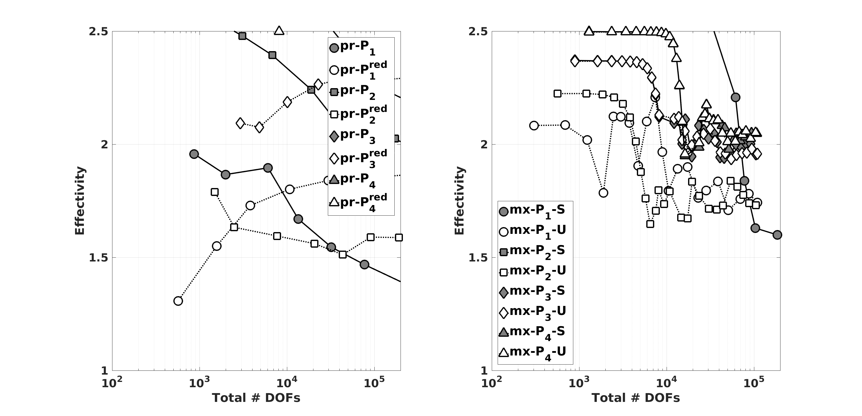 Figure 1
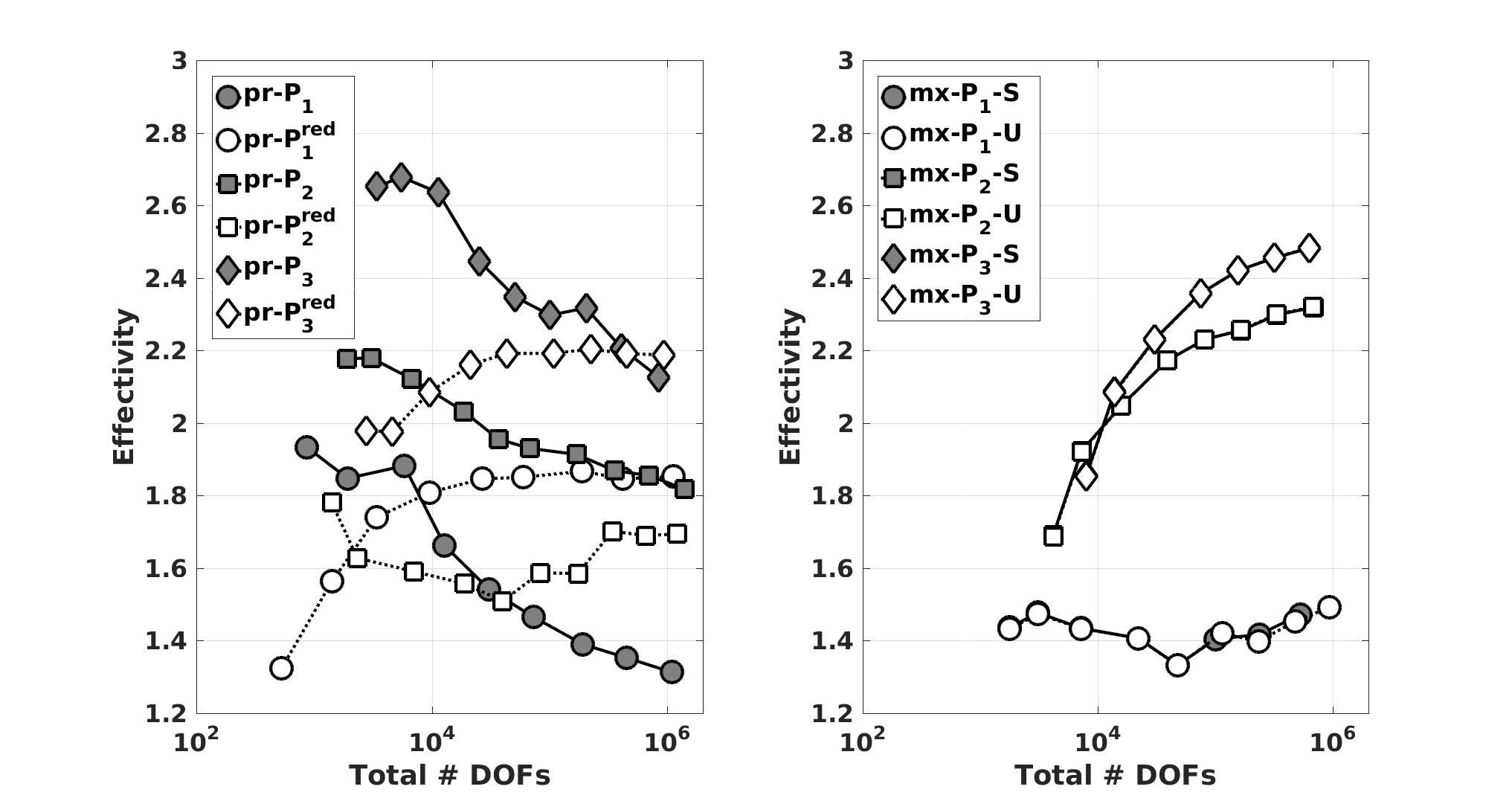 Figure 2
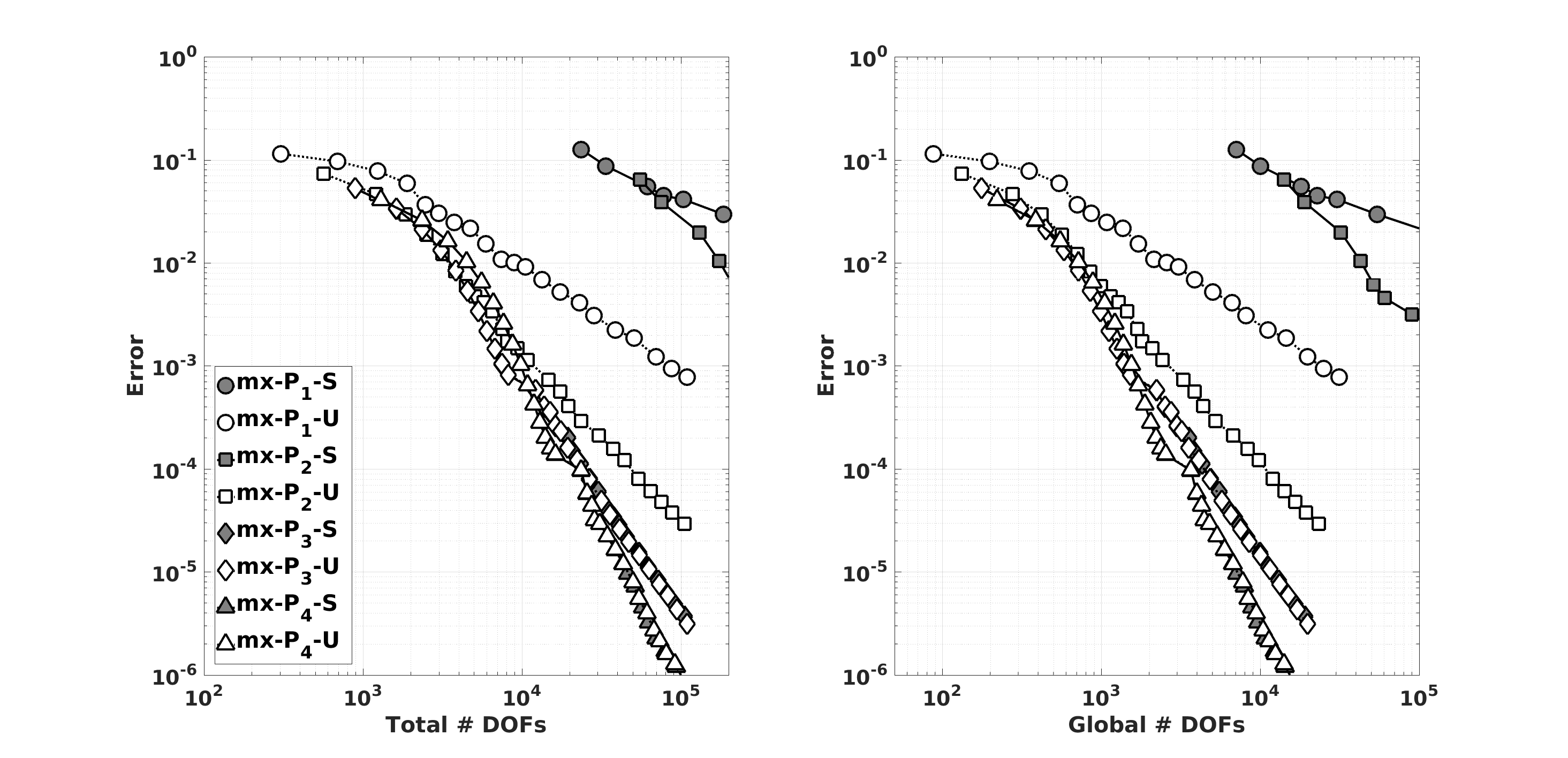 Figure 3
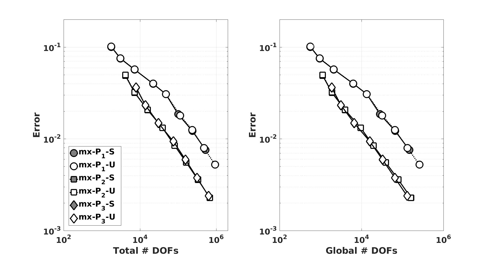 Figure 4
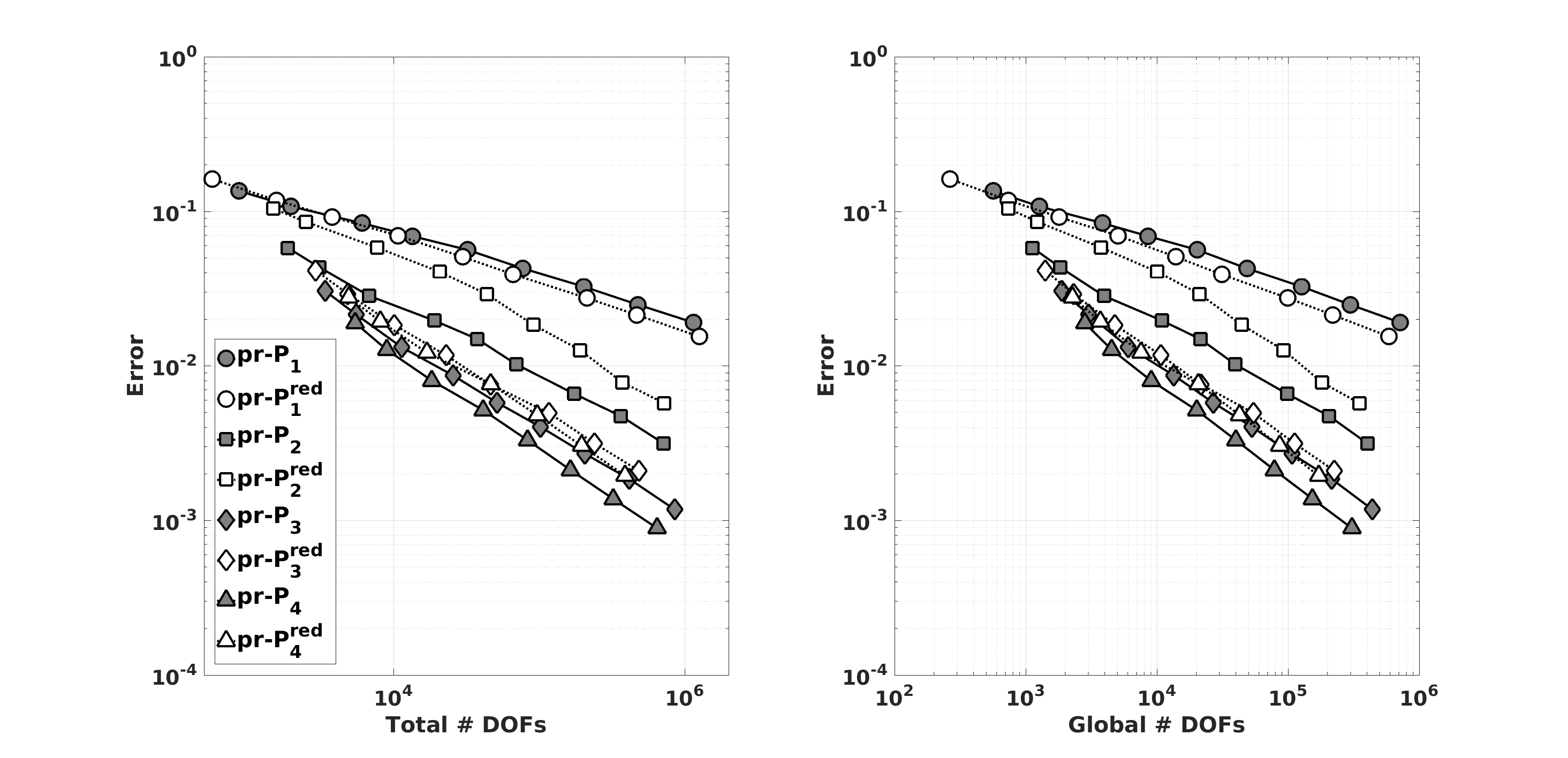 Figure 5
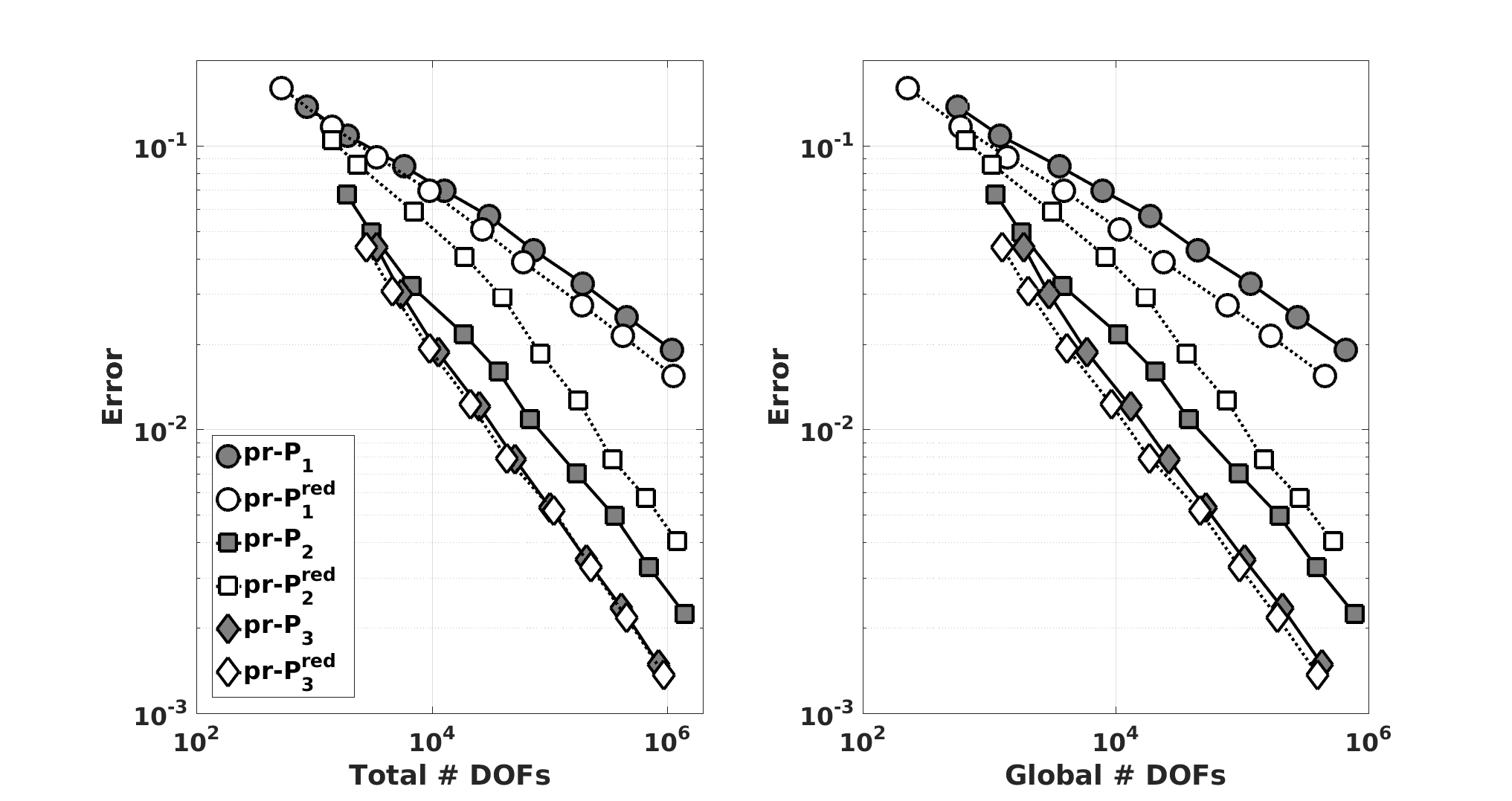 Figure 6
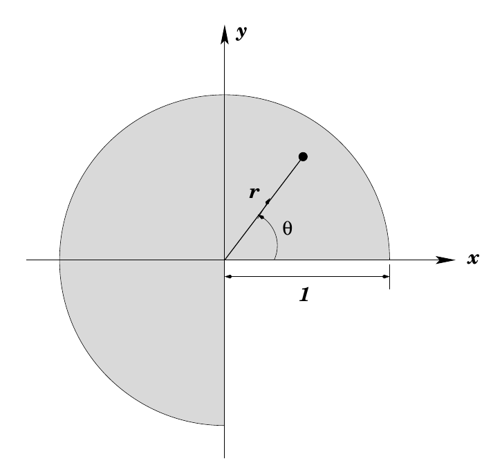 Figure 7
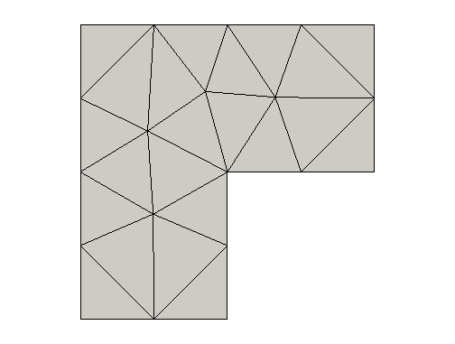 Figure 8
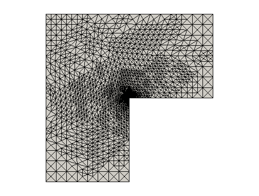 Figure 9
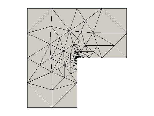 Figure 10
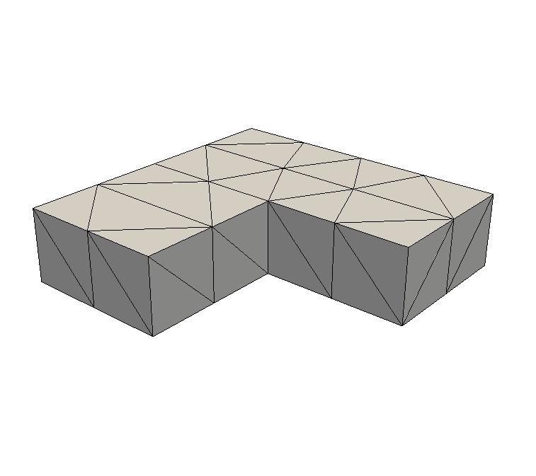 Figure 11
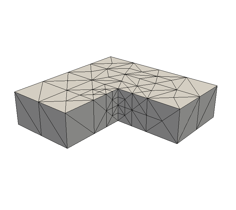 Figure 12
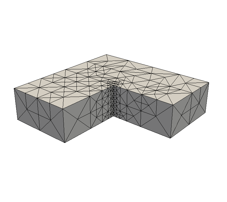 Figure 13
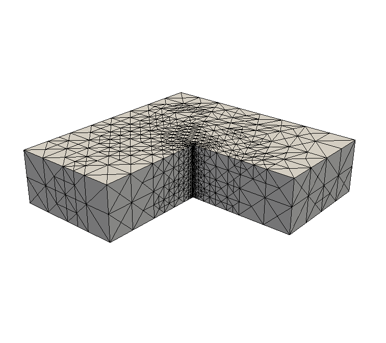 Figure 14
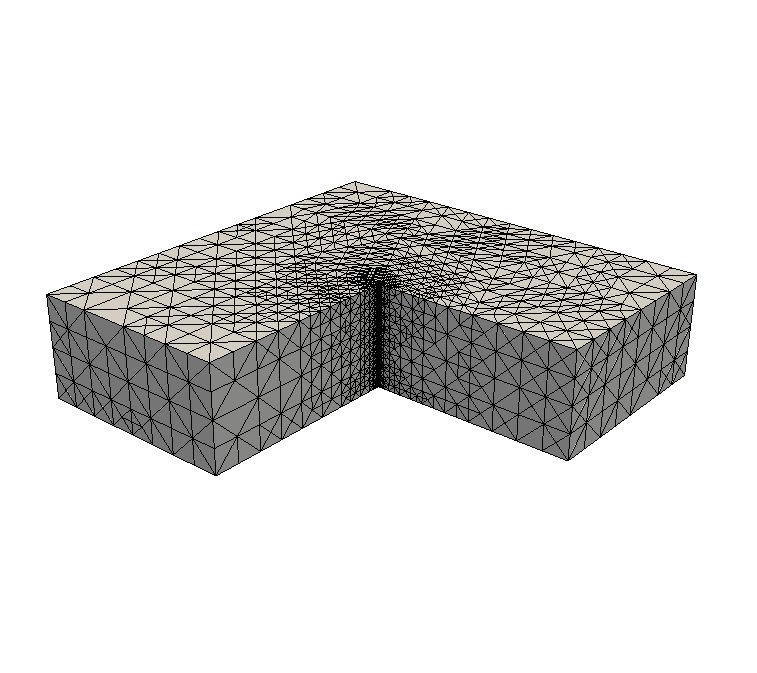 Figure 15
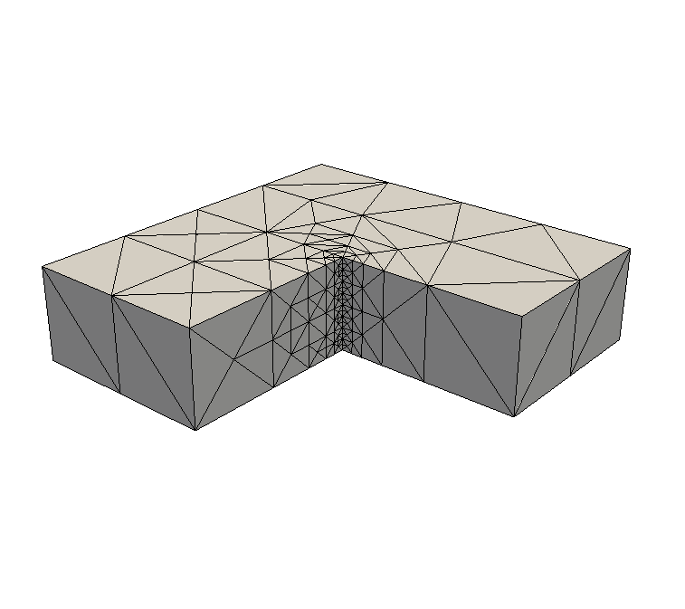 Figure 16
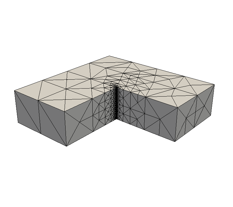 Figure 17
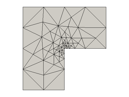 Figure 18
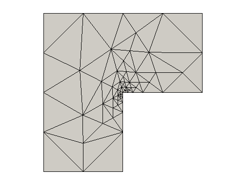 Figure 19
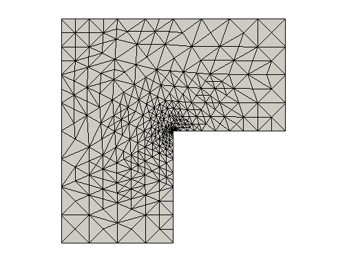 Figure 20
 Figure 21
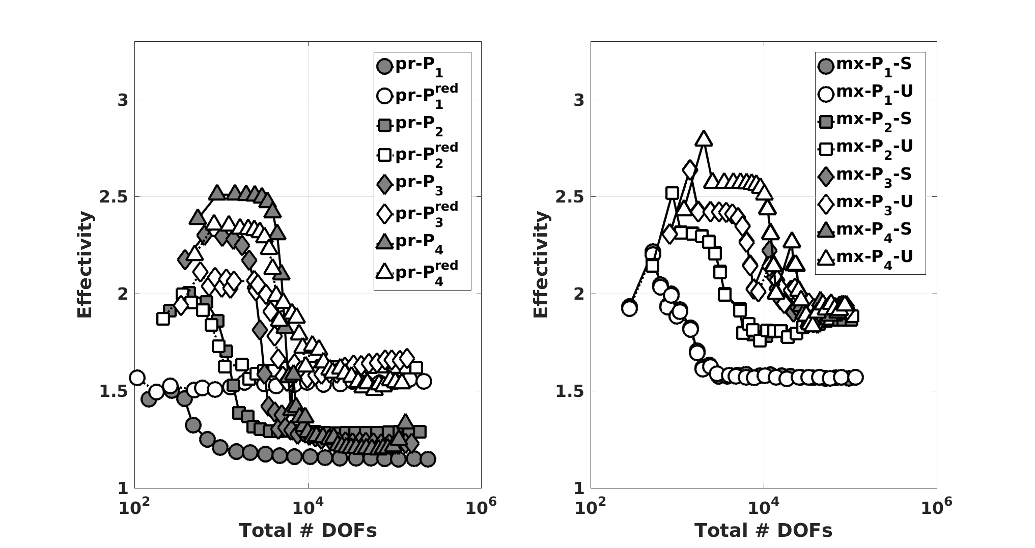 Figure 22
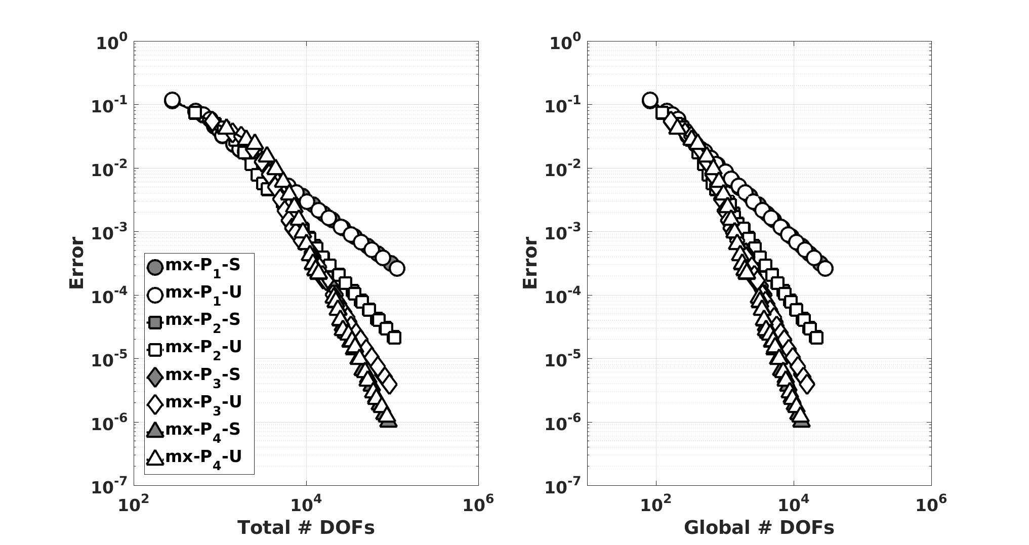 Figure 23
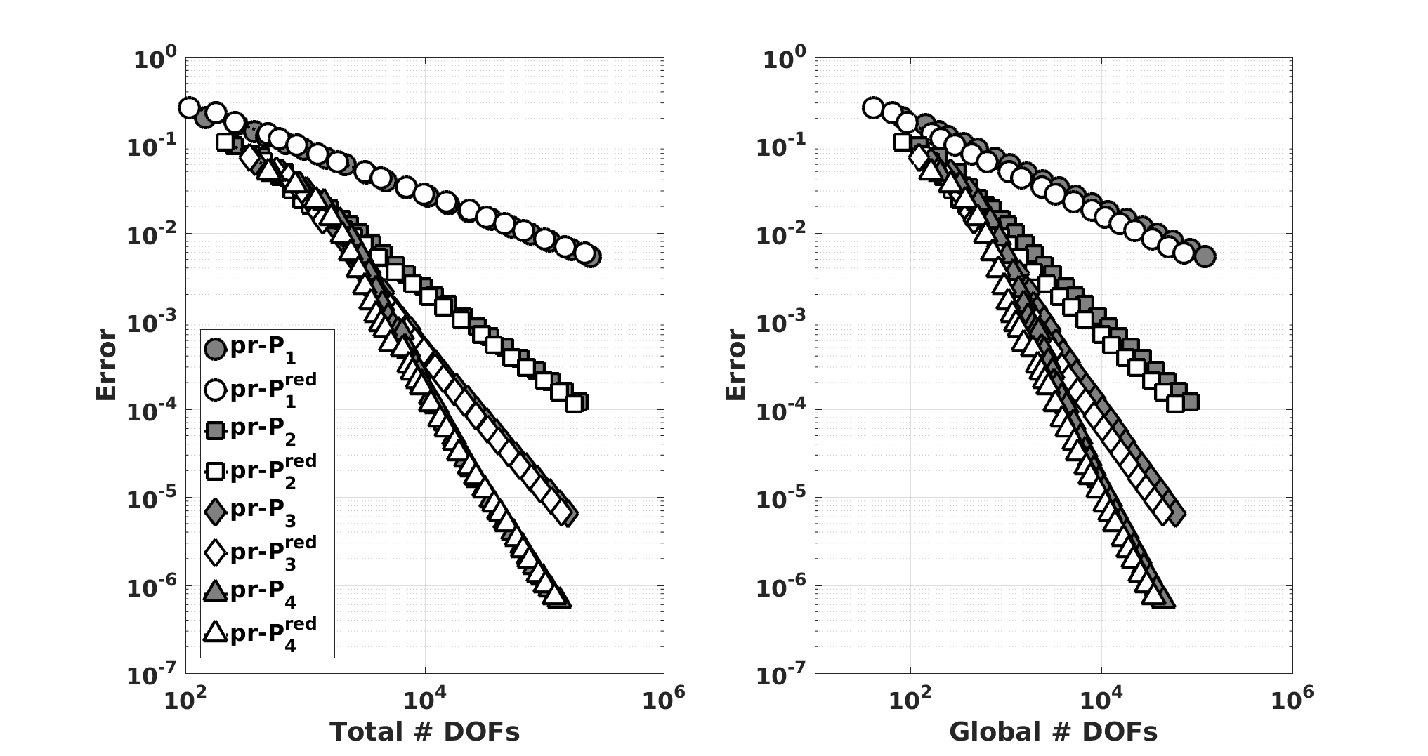 Figure 24
Peer Reviews
No public reviews on file for this paper yet. If you reviewed it on a platform where reviews are public (OpenReview, ICLR, NeurIPS, ICML), you can paste yours below so the community can read it here.
Videos
No videos yet. Explain this paper in a talk, walkthrough, or lecture? Add one.
Taxonomy
TopicsAdvanced Numerical Methods in Computational Mathematics · Numerical methods in engineering · Electromagnetic Simulation and Numerical Methods
Fully computable a posteriori error bounds for hybridizable discontinuous Galerkin finite element
approximations
Mark Ainsworth
Division of Applied Mathematics, Brown University, 182 George St, Providence RI 02912, USA.
and
Guosheng Fu
Division of Applied Mathematics, Brown University, 182 George St, Providence RI 02912, USA.
Abstract.
We derive a posteriori error estimates for the hybridizable discontinuous Galerkin (HDG) methods, including both the primal and mixed formulations, for the approximation of a linear second-order elliptic problem on conforming simplicial meshes in two and three dimensions.
We obtain fully computable, constant free, a posteriori error bounds on the broken energy seminorm and the HDG energy (semi)norm of the error. The estimators are also shown to provide local lower bounds for the HDG energy (semi)norm of the error up to a constant and a higher-order data oscillation term. For the primal HDG methods and mixed HDG methods with an appropriate choice of stabilization parameter, the estimators are also shown to provide a lower bound for the broken energy seminorm of the error up to a constant and a higher-order data oscillation term. Numerical examples are given illustrating the theoretical results.
Key words and phrases:
HDG, a posteriori error analysis, computable error bounds
1991 Mathematics Subject Classification:
65N30. 65Y20. 65D17. 68U07
First author gratefully acknowledges the partial support of this work under AFOSR contract FA9550-12-1-0399.
1. Introduction
Recent years have seen the developments of fully computable, guaranteed error bounds for the conforming [40, 37, 6, 7, 30, 42, 43, 14, 51, 18, 15], nonconforming [29, 1, 38, 39, 33, 19, 8], discontinuous Galerkin [2, 38, 39, 21, 9, 10], and mixed finite element methods [3, 38, 5, 27]; see also unified frameworks in [4, 16, 34].
In comparison, there are relatively few works on a posteriori error estimates for the hybridizable discontinuous Galerkin (HDG) methods [22]. The a posteriori estimates for HDG methods that are currently available in the literature [17, 25, 26, 31, 20, 35] are all of residual type, in which reliability is shown up to a generic (unknown) constant. This means that, while the associated estimation may be suitable as local refinement indicators, they cannot provide a quantitative stopping criterion. Moreover, if only a single fixed mesh is used (as is often the case in practice) then the value of an a posteriori bound containing unknown constants is somewhat questionable. Here we present, for the first time, fully computable a posteriori error bounds for HDG methods, for both the primal and mixed formulations, in the setting of a linear second-order elliptic problem on conforming simplicial meshes in two and three space dimensions. The key ingredient of our analysis is the local conservation property of the HDG methods, with which cheap element-wise equilibrated fluxes can be constructed.
The remainder of this article is organized as follows. Section 2 presents the model problem and prepares the notation used throughout the article. In Section 3, we introduce the primal HDG schemes and the corresponding computation error bounds. While in Section 4, we introduce the mixed HDG schemes and the corresponding computation error bounds. Numerical results are then presented in Section 5. The proofs of the main results in Section 3 and Section 4 are presented in Section 6.
2. Preliminaries
2.1. Model Problem
Consider the following model problem:
[TABLE]
subject to on , where , , is a simply connected polygonal/polyhedral domain. The datum is assumed to be strictly positive and, for simplicity, is assumed piecewise constant on subdomains of .
2.2. Notation and finite elements
We consider a family of partitions of the domain into the union of nonoverlapping, shape-regular, simplicial elements such that the nonempty intersection of a distinct pair of elements is a single common node, single common edge or single common face (in three dimensions). The family of partitions is assumed to be locally quasi-uniform in the sense that the ratio of the diameters of any pair of neighboring elements is uniformly bounded above and below over the whole family. Furthermore, it is assumed that the partitioning is compatible with the data so that is constant on each element.
The set of all facets (edges in two dimensions and faces in three dimensions) of the elements is denoted by , which we partition into subsets and consisting of facets lying on the boundary , and the remaining interior facets, respectively. Likewise, the corresponding quantities relative to an individual element are denoted by and , respectively. For each facet , the set consists of those elements for which is a facet,
[TABLE]
while, for each element , the set consists of those elements having a facet in common with ,
[TABLE]
Let denote the diameter of a domain , denote the measure of an element , denote the measure of a facet , and denote the measure of the boundary of an element .
Let , and denote the finite dimensional spaces
[TABLE]
To simplify notation, we introduce the compound finite-dimensional space
[TABLE]
which is used for the primal HDG scheme, while the compound finite-dimensional space
[TABLE]
is used for the mixed HDG scheme.
The stabilization parameters for the HDG schemes will be taken from the space , where, for any nonnegative integer ,
[TABLE]
with \mathbb{P}_{m}({{\partial K}}):=\{\mu\in L^{2}({\partial K}):\;\;\mu\raise-0.86108pt\hbox{|}_{F}\in\mathbb{P}_{m}(F)\;\;\forall F\in\mathcal{E}(K)\}.
We use the standard notation for jumps and averages [12] of functions in and on the mesh skeleton : Let be a facet shared by elements and with unit normal vectors and on pointing exterior to and respectively, then for
[TABLE]
We use the notation to denote the integral inner product over a region , and to denote the corresponding -norm. We omit the subscript in the case when is the physical domain . Finally, for each element , we use the notation to denote the integral inner product over the element boundary .
3. The primal HDG methods and computable error bounds
3.1. Primal HDG formulation
Let be a positive stabilization parameter to be specified later, and define the bilinear form by
[TABLE]
where denotes the projection onto the space . We also define the linear form by
[TABLE]
Let be the solution of (3). An approximation of (u,u\raise-0.86108pt\hbox{|}_{\mathcal{E}_{h}}) is obtained by seeking such that
[TABLE]
This scheme is known as the hybridized, symmetric, interior penalty discontinuous Galerkin method [41].
3.2. The choice of the stabilization
parameter .
It is well-known [41] that (13) is well-posed provided the stabilization parameter is “sufficiently large”. The following result quantifies exactly how large must be; similar results for interior penalty discontinuous Galerkin methods can be found in [48, 2, 32, 9, 10, 11].
Lemma 1**.**
Suppose the stabilization parameter is given by
[TABLE]
where is a constant satisfying
[TABLE]
Then (13) has a unique solution for and .
The proof of this and other results in this section is postponed to Section 6.
Remark 1**.**
*Observe that the stabilization parameter (14) on a facet is proportional to , which gives an optimal order a priori convergence rate in the energy norm [41, 44]. *
3.3. The broken energy seminorm and the HDG energy norm
For a given function , let the broken energy seminorm be denoted by
[TABLE]
Our objective is to derive a fully computable estimator for the error in the HDG finite-element approximation (e_{u},\widehat{e}_{u})=(u-u_{h},u\raise-0.86108pt\hbox{|}_{\mathcal{E}_{h}}-\widehat{u}_{h}), where is the solution to (3) and is the solution to (13). Let the HDG energy norm be denoted by
[TABLE]
Observe that, since , the quantity
[TABLE]
is directly computable in terms of the HDG approximation . Hence, given a constant free estimator for , we automatically have a constant free estimator for the HDG energy norm of the error as well. The next result shows that, by analogy with the standard interior penalty methods [2, 10], these norms are equivalent in the following sense.
Lemma 2**.**
Let the stabilization parameter be given by (14) with the global constant satisfying (15), then the HDG energy norm and the broken energy seminorm of the error (e_{u},\widehat{e}_{u})=(u-u_{h},u\raise-0.86108pt\hbox{|}_{\mathcal{E}_{h}}-\widehat{u}_{h}) are equivalent. That is to say,
[TABLE]
and there exists a positive constant , depending only on the shape-regularity of the mesh, the polynomial degree , and the local permeability ratio between neighboring elements, such that
[TABLE]
where the data oscillation on an element is defined to be
[TABLE]
The proof of this result is postponed to Section 6.
3.4. Local conservation
The numerical flux is defined by
[TABLE]
and satisfies the local conservation property
[TABLE]
along with
[TABLE]
These results are a straightforward consequence of the definition and (13).
3.5. The computable error bounds
We obtain computable error bounds for the discrete energy norm of the error by bounding the conforming and non-conforming errors separately [2, 10, 4]. To this end, two types of post-processing scheme will be needed.
3.5.1. Local (equilibrated) flux post-processing
We define a local flux post-processing [2, 9] as follows: Let be such that, on each element , there holds
[TABLE]
where
[TABLE]
denotes the divergence-free “bubble” space. The unique solvability of (24) can be established using arguments similar to those used to study the closely related Brezzi-Douglas-Marini (BDM) projection [13]. By the local conservation properties (22) and (23), we conclude that satisfies
[TABLE]
The quantity is usually referred to as an equilibrated flux [7].
3.5.2. Local potential post-processing
We obtain a globally continuous potential by a simple averaging [2, 10] of the discontinuous potential as follows: Let index a set of points on associated with a Lagrange basis for the conforming finite-element space of order on and let denote the restriction of the set to the points that do not lie on the boundary of element , with being its complementary set. Let denote the restriction of the set to the points that lie on the closure of the boundary . For , let denote the set of elements in whose closure contains the point .
The post-processed potential is obtained through a simple averaging of the degrees of freedom for : for all elements , u_{h}^{*}\raise-0.86108pt\hbox{|}_{K}=S_{k}(u_{h})\raise-0.86108pt\hbox{|}_{K}\in\mathbb{P}_{k}(K), where the nodal values are given by
[TABLE]
and denotes the number of elements of contained in the patch .
3.5.3. Computable error bounds
The foregoing developments show that each of the quantities
[TABLE]
can be computed directly from the primal HDG approximation using purely local computations. The next result shows that together these quantities provide a computable, constant-free, upper bound on the broken energy seminorm of the error:
Theorem 1**.**
*Let and be defined as in (31), and let the stabilization parameter be of the form (14) where satisfies (15). Then *
[TABLE]
Moreover, there exists a positive constant , depending only on the shape-regularity of the mesh, the polynomial degree , and the local permeability ratio between neighboring elements, such that
[TABLE]
Furthermore,
[TABLE]
and
[TABLE]
where is as above.
The proof of this result is similar to [2, Theorem 2] and an outline of the main steps is given in Section 6 below. Numerical examples illustrating the bounds in practice are given in Section 5.
4. The mixed HDG methods and computable error bounds
4.1. The mixed HDG formulation
Whereas the primal HDG method gives an approximation for (u,u\raise-0.86108pt\hbox{|}_{\mathcal{E}_{h}}), the mixed HDG method seeks, in addition, to approximate the flux (a{\nabla}u,u,u\raise-0.86108pt\hbox{|}_{\mathcal{E}_{h}}).
Let be a positive stabilization parameter to be specified later, and define the bilinear form by
[TABLE]
along with the linear form by
[TABLE]
An approximation of the true solution (a{\nabla}u,u,u\raise-0.86108pt\hbox{|}_{\mathcal{E}_{h}}) is obtained by seeking such that
[TABLE]
This scheme was originally termed the local discontinuous Galerkin-hybridizable method (LDG-H) [22] but is referred to here as the mixed HDG approximation.
4.2. The choice of the stabilization
parameter .
The mixed HDG scheme enjoys greater stability properties than the primal HDG scheme as the stabilization parameter need only be (partially) positive in order for the scheme to be well-posed as the following result [22, Proposition 3.2] shows.
Lemma 3**.**
If the nonnegative stabilization parameter is chosen such that on at least one facet for every element , then there exists a unique solution for .
Remark 2** (Stabilization parameter).**
The two most common choices of stabilization parameter used in practice are:
- •
uniform stabilization
[TABLE]
- •
single-facet stabilization
[TABLE]
where is an arbitrarily chosen but fixed facet of .
Each of the above choices of stabilization parameters results in an optimal a priori convergence rate of the error in the energy norm [23].
4.2.1. The broken energy seminorm and the HDG energy seminorm
For a given function , let the broken energy seminorm be denoted by
[TABLE]
and let the mixed HDG energy seminorm be denoted by
[TABLE]
The error in the mixed HDG finite-element approximation is denoted by ({\boldsymbol{e}}_{\sigma},e_{u},\widehat{e}_{u})=({\boldsymbol{\sigma}}-{\boldsymbol{\sigma}}_{h},u-u_{h},u\raise-0.86108pt\hbox{|}_{\mathcal{E}_{h}}-\widehat{u}_{h}), where is the solution to (3) and is the solution to (36). Similarly to the primal HDG case, we have and hence the quantity
[TABLE]
can be evaluated directly given the mixed HDG approximation. Consequently, given a constant free estimator for the broken energy seminorm of the error, we automatically have a constant free estimator for the HDG energy seminorm of the error as well. The next result shows that, by analogy with the primal HDG case, the HDG energy seminorm of the error is equivalent to the broken energy seminorm when the single-facet stabilization (37d) is used.
However, the equivalence fails to hold if the uniform stabilization (37a) is employed. For instance, in the case of lowest order () approximation, the discrete energy norm (plus the data oscillation) cannot control the jump term as shown by the counterexample constructed in [24, Section 2.4.1]. The situation for general remains an open problem at this time.
Lemma 4**.**
Let the stabilization parameter given by (37d), then the HDG energy seminorm and the broken energy seminorm of the error ({\boldsymbol{e}}_{\sigma},e_{u},\widehat{e}_{u})=({\boldsymbol{\sigma}}-{\boldsymbol{\sigma}}_{h},u-u_{h},u\raise-0.86108pt\hbox{|}_{\mathcal{E}_{h}}-\widehat{u}_{h}) are equivalent in the sense that
[TABLE]
*and there exists a positive constant , depending only on the shape-regularity of the mesh and the polynomial degree , such that *
[TABLE]
Proof.
The result follows at once from Lemma 7 in Section 6 below. ∎
4.3. Local conservation
Similarly to the primal HDG scheme (13), the mixed HDG scheme (36) is locally conservative but this time in the sense that the numerical flux
[TABLE]
satisfies
[TABLE]
along with
[TABLE]
4.4. The computable error bounds
We are now in a position to present computable error bounds for the discrete energy error. While the basic approach is motivated by the technique used in [3, 5, 27] for the mixed methods, the post-processing technique needed for the mixed HDG case is quite different.
4.4.1. Local (equilibrated) flux post-processing
Let satisfy the following conditions, on each element :
[TABLE]
Thanks to the local conservation properties (22) and (23), we conclude that satisfies
[TABLE]
4.4.2. Local potential post-processing
A global continuous potential is constructed by averaging a higher order discontinuous approximation to the potential. However, the averaging scheme is more involved than the one used in the primal case: Firstly, we find so that, on each element , there holds
[TABLE]
The continuous potential post-processing is then a simple averaging of the degrees of freedom for , where is defined as in (30).
4.4.3. Computable error bounds
Each of the quantities
[TABLE]
can be computed directly from the mixed HDG approximation using only local computations. These quantities provide computable, constant-free, upper bounds on the the broken energy seminorm of the error :
Theorem 2**.**
*Let and be defined as in (31), with the stabilization parameter chosen to be either (37a) or (37d). Then *
[TABLE]
*Moreover, there exists a positive constant , depending only on the shape-regularity of the mesh, the polynomial degree , and the local permeability ratio between neighboring elements, such that *
[TABLE]
where is an arbitrary but fixed facet of . Furthermore,
[TABLE]
with
[TABLE]
The proof of Theorem 2 is presented in Section 6.
Remark 3** (Single-facet stabilization).**
If the stabilization parameter is chosen as in (37d), then we can take in (48) to be the unique facet on which is non-zero which implies that
[TABLE]
Consequently, for the choice (37d), the estimator also gives a lower bound for the broken energy seminorm.
5. Numerical examples
In order to illustrate the results in Theorem 1–2, we consider Poisson problems in two and three dimensions approximated using the primal and mixed HDG schemes (13) and (36). The implementation is performed using the Python interface of the NGSolve software [46, 47]. Conveniently, NGSolve provides a set of basis functions for the divergence-free bubble space (25) [45] which makes the implementation of the equilibrated flux reconstructions (24) and (44) relatively straightforward.
We choose the stabilization parameter for the primal HDG schemes (13) to be
[TABLE]
which, thanks to Lemma 1, ensures well-posedness on shape-regular meshes. We adopt a shorthand notation and denote the primal HDG scheme (13) used in conjunction with the approximation space as pr-Pk, while if with the approximation space used we use the notation: pr-P. Likewise, we denote the mixed HDG scheme (36) used in conjunction with uniform stabilization (37a) as mx-Pk-U, while if the single-facet stabilization (37d) is used, we write mx-Pk-S. In all cases we use static condensation whereby the local, cell-wise, degrees of freedom are eliminated leaving only those degrees of freedom which are located on the mesh skeleton.
We take polynomial degree for the first example, and for the second example.
5.1. Example 1: Two-dimensional L-shaped problem
Here we consider the Laplace problem on a planar L-shaped domain with Dirichlet boundary conditions. The initial mesh is shown in Fig. 1(A). The true solution is given by in polar coordinates.
The sequence of meshes was constructed by selecting for refinement the smallest number of elements whose combined contribution toward the estimator of the broken energy seminorm of the error exceeds half of the total estimated error. A sample of the meshes for the pr-Pk scheme with and is shown in Fig. 2.
In Fig. 3, we plot the error for the primal scheme in the broken energy seminorm (16) against the total number of degrees of freedom and the number of global degrees of freedom, , remaining after local variables have been eliminated. The error in the broken energy seminorm (38) for the mixed HDG schemes is shown in Fig. 4.
In all cases, the effectivity indices are found to lie in the range – as shown in Fig 5.
5.2. Example 2: Three-dimensional L-shaped problem
Here we consider the Laplace problem on a three-dimensional L-shaped domain , where is the two-dimensional L-shaped domain in the previous example. The initial mesh is shown in Fig. 1(B). The true solution is independent of , and reduces to the same two-dimensional solution as Example 1. However, the fact that the true solution is independent of is not used in the finite element analysis and the meshes are unstructured through the thickness.
A sample of the meshes obtained for adaptive solution using the pr-Pk scheme with and is shown in Fig. 6. The errors for the primal and mixed HDG schemes are plotted in Fig. 7 and Fig. 8, respectively. As before, the effectivity indices are found to vary in the range – as shown in Fig. 9.
6. Proofs
We now turn to the proofs of the results.
As remarked earlier, the jump term in the HDG energy (semi)norm is directly computable, and, as such, we need only concern ourselves with obtaining estimates for the broken energy seminorm of the error. To this end, recall the following Helmholtz decomposition [36, 28]:
Lemma 5**.**
Let be a simply connected polygon/polyhedron. Then, any , , can be written in the form
[TABLE]
where satisfies
[TABLE]
and satisfies
[TABLE]
Moreover, the decomposition is orthogonal
[TABLE]
We shall use the decomposition (50) in conjunction with defined elementwise by for the primal HDG scheme (13), or by for the mixed HDG scheme (36). In both cases, Lemma 5 gives an orthogonal decomposition of the broken energy seminorm error into the sum of a conforming part and a nonconforming part . It then suffices to obtain an a posteriori error bound for each part separately and sum to obtain an estimator for the total error.
6.1. Proof of Theorem 1
The proof of Theorem 1 follows from [10] for the symmetric interior penalty discontinuous Galerkin methods almost verbatim. Specifically, the upper bound (32) in Theorem 1 follows from (54a) and (54b) below, and the lower bound (33) follows from Lemma 2, (54) and (54d).
The following estimates follows from results in [10, Lemma 6.2-6.5] using the proof in [9, Section 6]. Let and be taken as in (50) in the case where , and let and be given by (31). Then,
[TABLE]
where .
6.2. Proof of Theorem 2
Theorem 2 is a consequence of the following three lemmas:
Lemma 6**.**
Let and be given by in the decomposition (50), where is chosen to be , and let and be given by (47). Then,
[TABLE]
where
Proof.
Direct computation gives
[TABLE]
where the last inequality follows from the Cauchy-Schwarz and the Poincaré inequalities. This completes the proof of (55a). Turning to (55b), since for all , we have
[TABLE]
Let , then for all , by (44), we have satisfies
[TABLE]
Hence, there exists a constant , depending only on the polynomial degree and shape-regularity of the element , such that
[TABLE]
while, using a standard bubble function technique [7, 50], we have
[TABLE]
The choice of stabilization parameter (37) means that
[TABLE]
and the proof of (55) follows from these estimates.
Finally, we have
[TABLE]
Combining the above estimates completes the proof of (55d). ∎
Lemma 7**.**
There exists a positive constant , depending only on the shape-regularity of the mesh and the polynomial degree , such that for any facet ,
[TABLE]
Proof.
The mixed HDG scheme (36) satisfies, for every ,
[TABLE]
Let the function satisfy
[TABLE]
where is a fixed facet of . We have, by a standard scaling argument,
[TABLE]
Taking in (59) and rearranging terms, we obtain
[TABLE]
The proof is completed by invoking estimate (57) for the cell-wise residual term . ∎
Lemma 8**.**
*There exists a positive constant , depending only on the shape-regularity of the mesh and the polynomial degree , such that *
[TABLE]
Proof.
We first prove the estimate (60). We denote and let the function be defined as follows:
[TABLE]
then, we have
[TABLE]
Moreover, by equations (46a) and (62), we have
[TABLE]
This implies that because . Since has vanishing normal trace on by equations (62a), we obtain
[TABLE]
Hence,
[TABLE]
The estimate (60) now follows from the Cauchy-Schwarz inequality.
Let be the -projection onto the space . Applying the results in [27, Lemma 3.4-3.5], we obtain
[TABLE]
The estimate (61) now immediately follows from the triangle inequality and (60).
∎
6.3. Proof of Lemma 1
Since is a finite-dimensional space, it suffices to show that is the only solution to the homogeneous problem. Let
[TABLE]
then for , we have
[TABLE]
Since a{\nabla}v_{h}\cdot{\boldsymbol{n}}\raise-0.86108pt\hbox{|}_{F}\in\mathbb{P}_{k-1}(F), there holds
[TABLE]
By the Cauchy-Schwarz and Young’s inequalities, for any ,
[TABLE]
where, the final inequality holds thanks to the inverse-trace inequality [52] and a{\nabla}u\raise-0.86108pt\hbox{|}_{K}\in\mathbb{P}_{k-1}(K)^{d}. Summing the above inequality over gives
[TABLE]
Hence, we have
[TABLE]
Finally, if satisfies (15) then there exists an such that
[TABLE]
Consequently, when the right hand side of (13) vanishes, for all and for all . Hence, the only solution to the homogeneous problem is , and therefore there exists a unique solution to (13).
6.4. Proof of Lemma 2
The proof follows that of [2, Theorem 3].
By the conservation property (23), we have
[TABLE]
Hence,
[TABLE]
Inserting the above expression into the jump term in the HDG energy norm and regrouping gives
[TABLE]
Here, the gradient jump term can be controlled by the standard bubble function technique [50, 7]
[TABLE]
On the other hand, there holds
[TABLE]
where denote the average value of on the facet . Thanks to the trace and Poincaré inequalites, we have
[TABLE]
Hence, to show norm equivalence, it remains to show that the term
[TABLE]
can be controlled by the discrete energy seminorm plus the data oscillation. Replacing in the primal HDG scheme (13) with the expression (66), we obtain
[TABLE]
for all and .
Moreover, there holds [49]
[TABLE]
where is the element stiffness matrix, i.e. with being the barycentric coordinates for the element , and is its spectral radius. Hence the stabilization parameter in (14), with satisfying (15), satisfies
[TABLE]
The proof is then concluded following [2, Theorem 3] by taking special linear test functions in the equation (6.4) and using the above estimate for the stabilization parameter.
The reference list from the paper itself. Each links out to its DOI / PubMed record.
- 1[1] M. Ainsworth , Robust a posteriori error estimation for nonconforming finite element approximation , SIAM J. Numer. Anal., 42 (2005), pp. 2320–2341.
- 2[2] , A posteriori error estimation for discontinuous Galerkin finite element approximation , SIAM J. Numer. Anal., 45 (2007), pp. 1777–1798.
- 3[3] , A posteriori error estimation for lowest order Raviart-Thomas mixed finite elements , SIAM J. Sci. Comput., 30 (2007/08), pp. 189–204.
- 4[4] , A framework for obtaining guaranteed error bounds for finite element approximations , J. Comput. Appl. Math., 234 (2010), pp. 2618–2632.
- 5[5] M. Ainsworth and X. Ma , Non-uniform order mixed FEM approximation: implementation, post-processing, computable error bound and adaptivity , J. Comput. Phys., 231 (2012), pp. 436–453.
- 6[6] M. Ainsworth and J. T. Oden , A unified approach to a posteriori error estimation using element residual methods , Numer. Math., 65 (1993), pp. 23–50.
- 7[7] , A posteriori error estimation in finite element analysis , Pure and Applied Mathematics (New York), Wiley-Interscience [John Wiley & Sons], New York, 2000.
- 8[8] M. Ainsworth and R. Rankin , Fully computable bounds for the error in nonconforming finite element approximations of arbitrary order on triangular elements , SIAM J. Numer. Anal., 46 (2008), pp. 3207–3232.