Double jump phase transition in a soliton cellular automaton
Lionel Levine, Hanbaek Lyu, John Pike

TL;DR
This paper analyzes a soliton cellular automaton with random initial states, revealing phase transitions in soliton sizes and uncovering a condensation phenomenon, with implications for permutation subsequences and connections to stochastic processes.
Contribution
It provides new constructions of Young diagrams for the automaton, establishes limit theorems for soliton sizes, and uncovers a phase transition and condensation phenomena.
Findings
Number of solitons scales linearly with system size n.
Longest soliton length scales as log n, √n, or n depending on p.
Condensation occurs in the supercritical regime for p > 1/2.
Abstract
In this paper, we consider the soliton cellular automaton introduced in [Takahashi 1990] with a random initial configuration. We give multiple constructions of a Young diagram describing various statistics of the system in terms of familiar objects like birth-and-death chains and Galton-Watson forests. Using these ideas, we establish limit theorems showing that if the first boxes are occupied independently with probability , then the number of solitons is of order for all , and the length of the longest soliton is of order for , order for , and order for . Additionally, we uncover a condensation phenomenon in the supercritical regime: For each fixed , the top soliton lengths have the same order as the longest for , whereas all but the longest have order at most for . As an…
Click any figure to enlarge with its caption.
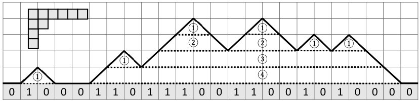 Figure 1
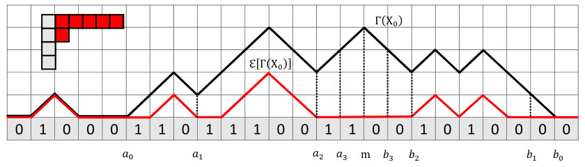 Figure 2
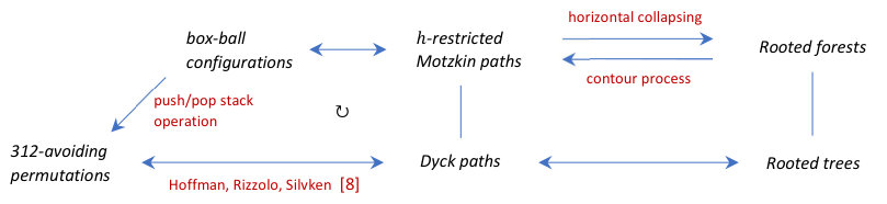 Figure 3
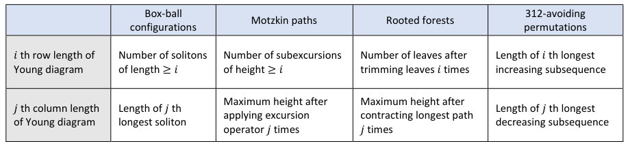 Figure 4
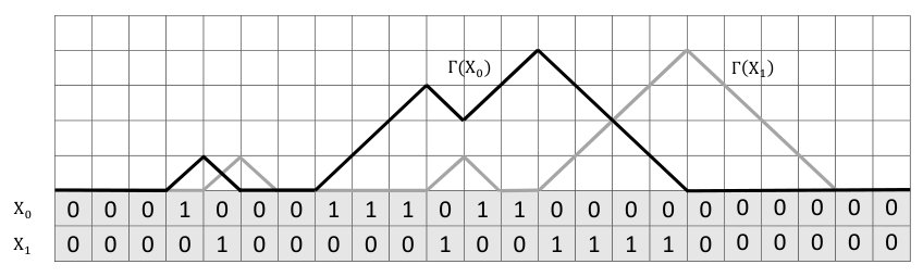 Figure 5
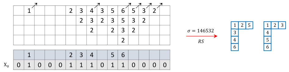 Figure 6
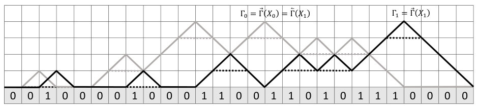 Figure 7
 Figure 8
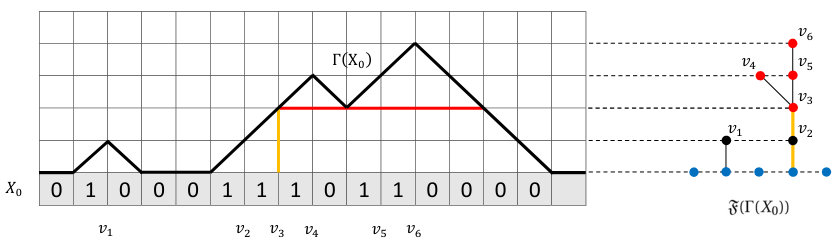 Figure 9
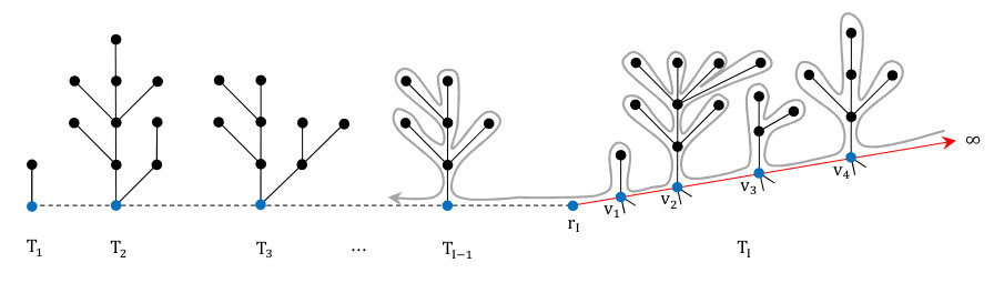 Figure 10
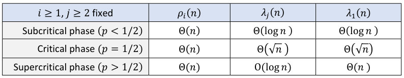 Figure 11
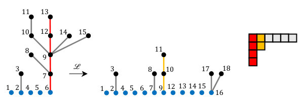 Figure 12
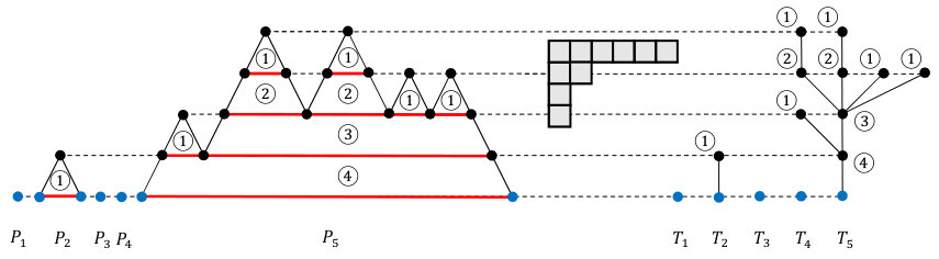 Figure 13
Peer Reviews
No public reviews on file for this paper yet. If you reviewed it on a platform where reviews are public (OpenReview, ICLR, NeurIPS, ICML), you can paste yours below so the community can read it here.
Videos
No videos yet. Explain this paper in a talk, walkthrough, or lecture? Add one.
Double jump phase transition in a soliton cellular automaton
Lionel Levine
Lionel Levine, Department of Mathematics, Cornell University, Ithaca, NY 14853.
,
Hanbaek Lyu
Hanbaek Lyu, Department of Mathematics, University of California, Los Angeles, CA 90095.
and
John Pike
John Pike, Department of Mathematics, Bridgewater State University, Bridgewater, MA 02324.
(Date: March 13, 2024)
Abstract.
In this paper, we consider the soliton cellular automaton introduced in [25] with a random initial configuration. We give multiple constructions of a Young diagram describing various statistics of the system in terms of familiar objects like birth-and-death chains and Galton-Watson forests. Using these ideas, we establish limit theorems showing that if the first boxes are occupied independently with probability , then the number of solitons is of order for all , and the length of the longest soliton is of order for , order for , and order for . Additionally, we uncover a condensation phenomenon in the supercritical regime: For each fixed , the top soliton lengths have the same order as the longest for , whereas all but the longest have order for . As an application, we obtain scaling limits for the lengths of the longest increasing and decreasing subsequences in a random stack-sortable permutation of length in terms of random walks and Brownian excursions.
Key words and phrases:
box-ball system, phase transition, condensation, excursion operator, birth-death chain, Motzkin path, Galton-Watson forest, Brownian motion, random stack-sortable permutation
2010 Mathematics Subject Classification:
37K40, 60F05
1. Introduction
In 1990, Takahashi and Satsuma proposed a dimensional cellular automaton of filter type called the soliton cellular automaton, also known as the box-ball system [17, 25]. It is defined as a discrete-time dynamical system whose states are binary sequences with finitely many ’s. We may think of the states as configurations of balls in boxes where box contains a ball at stage if and is empty if . The update rule is defined as follows: At the beginning of stage , each ball has been moved a total of times. To reach stage , successively move the leftmost ball which has been moved a total of times to the first empty box on its right, continuing until all balls have been moved. Alternatively, at each stage a ‘carrier’ starts at the origin and sweeps rightward to infinity. Each time she encounters an occupied box, she pushes the ball to the top of her stack. Each time she encounters an empty box and her stack is nonempty, she pops any ball from her stack into the box. In keeping with this picture, we will refer to the stages of the box-ball system as sweeps henceforth.
As a concrete example, the system initially having balls in boxes evolves through sweep as
[TABLE]
In this model, a (non-interacting) soliton of length is defined to be a string of consecutive ’s followed by consecutive [math]’s. During one sweep, such a soliton travels to the right at speed . The physical interpretation is that of a traveling wave with velocity equal to its wavelength. If a -soliton precedes a -soliton with , then the two will eventually collide, resulting in interference. The subsequent states of the system depend on the congruence class of their initial distance modulo their relative speed, , but solitons are never created or destroyed in the course of these interactions. The case of three or more interacting solitons can be described similarly [25]. It is easy to see that since we have finitely many balls initially, after some finite time the system consists of non-interacting solitons whose lengths are nondecreasing from left to right. We will call such a configuration stable. This final macrostate of the system can be encoded in the Young diagram having column equal in length to the longest soliton.
In this paper, we start the soliton cellular automaton from a random initial configuration and study the limiting shape of the resulting Young diagram. We have two parameters, and . Let be a random coloring of so that each site in is with probability and [math] with probability , independently of all others, and all sites in are [math]. Let be the corresponding random Young diagram and denote the lengths of its row and column by and , respectively. (Thus gives the length of the longest soliton and the number of solitons of length at least .) We are going to show that each fixed row has order for all values of , but the column lengths vary drastically according to whether is less than, equal to, or greater than . The asymptotics of the rows and columns of are summarized in the following table, for which Theorem 1 proves the entries, and Theorem 2 proves the entries. For the precise meaning of the Landau notation employed, see Subsection 1.2.
Erdős and Rényi coined the term double jump to describe the emergence of a giant component in the sparse random graph with vertices, each pair independently joined by an edge with probability , where is a parameter. The analogy between random graph components and box-ball solitons becomes apparent if we take . Then with high probability, all connected components of the Erdős-Rényi graph are of size for ; components of size emerge at ; and for , the largest component is of size while all the rest have size [8]. Except for the exponent (which becomes ) this is exactly the behavior of the soliton lengths in the box-ball system as summarized in the last two columns of Table 1.
1.1. Related work
There have been some exciting recent developments involving the box-ball system with a bi-infinite random initial configuration. A central question is to understand the invariant measures on under the box-ball dynamics. Ferrari, Nguyen, Rolla, and Wang [9] showed that the Bernoulli product measure with density is invariant and provided a recipe for constructing additional invariant measures based on a soliton decomposition of box-ball configurations. Croydon, Kato, Sasada, and Tsujimoto [4] found sufficient conditions for invariance using Pitman’s transformation and considered extending the box-ball system from to . See the references for more details.
1.2. Notation
We adopt the notation , , and throughout. We employ the Landau notation in the sense of stochastic boundedness. That is, given and a sequence of nonnegative random variables, we say that if for every , there is a such that for all . We say that if for every , there is a such that for all , and we say if and . The constants may depend on and but not .
1.3. Main results
Fix , and let be a sequence of i.i.d. random variables with law and . Define by
[TABLE]
and for each , set . The interpretation is that corresponds to an arrangement of balls in boxes where boxes are each occupied independently with probability , and boxes are empty.
For each fixed and , we consider the box-ball system with the random initial configuration . Recall that the soliton lengths are denoted by . This information can be summarized by the Young diagram whose column has length . The length of its row, , equals the number of solitons in the system having length at least . In particular, gives the total number of solitons.
Many properties of this Young diagram can be described in terms of the simple random walk defined by and . Our first result shows that the longest rows are of order for any .
Theorem 1**.**
Let and be as above. Then the following statements hold.
(i)
(SLLN for rows) Let be the first return time of to [math]. Then for any fixed ,
[TABLE]
(ii)
(CLT for the first row)
[TABLE]
where , the standard normal distribution.
Denote by the space of continuous functions endowed with the topology of uniform convergence on compact sets, and let be the subspace of consisting of nonnegative compactly supported functions such that on . For any closed interval containing [math], denote by and the space of restrictions where and , respectively. For , define the operator by
[TABLE]
where and . We call the pivot of . Define by , the location of the rightmost global maximum of . Finally, define the excursion operator on by . See Figure 4 for an illustration.
We now state the main result of the paper.
Theorem 2**.**
Let be as above and set . Let denote the longest soliton length.
(i)
(Subcritical phase) For , is concentrated around for each fixed in the sense that for all ,
[TABLE]
In particular, .
(ii)
(Critical phase) For , let be a standard Brownian motion on . Then for each fixed ,
[TABLE]
In particular, .
Furthermore, for any integers ,
[TABLE]
(iii)
(Supercritical phase) For ,
[TABLE]
Furthermore, there exists a constant such that
[TABLE]
and for all , is concentrated around in the sense that for all ,
[TABLE]
In particular, and if .
We call the statement in Theorem 2 (iii) a condensation phenomenon because in the supercritical regime, a linear number of balls condense into the longest soliton while the next longest solitons each have balls.
The methods that we develop in this paper to study the box-ball system yield several interesting results on lengths of monotone subsequences in random pattern avoiding permutations. The study of statistics involving longest increasing or decreasing subsequences in different types of random permutations has a long history and rich connections to many other fields [22]. In the context of the box-ball system, the class of -avoiding permutations arises naturally, and we are able to generalize some classical results on such permutations in multiple directions.
For each , let be the set of all permutations on . Given two permutations and with , we say that is -avoiding if no subsequence of has the same relative order as . (For example, a permutation is -avoiding if there is no subsequence of the form with .) Denote by the set of all -avoiding permutations in . Note that is -avoiding if and only if is -avoiding. (In particular, is 231-avoiding if and only if is 312-avoiding.) Given a permutation , define integers (resp. ) recursively so that (resp. ) equals the length of the longest subsequence in obtained by taking a disjoint union of decreasing (resp. increasing) subsequences.
In a classic work [23], Rotem studied properties of 231-avoiding permutations chosen uniformly at random among all such permutations of a given length. He showed that if is a permutation in chosen uniformly at random, then
[TABLE]
Our next theorem is an extension of the above result both to the higher moments and to ‘subsequent’ longest increasing and decreasing subsequences of .
Theorem 3**.**
Let be a uniformly chosen random - (or -) avoiding permutation of length .
(i)
Suppose that is a sequence of rooted trees where is chosen uniformly at random among all rooted plane trees on nodes, and for , is obtained from by deleting all leaves. Then
[TABLE]
(ii)
Let be a simple symmetric random walk with and let be the time of its first return to [math]. Then for any fixed ,
[TABLE]
(iii)
Let be a standard Brownian excursion on . Then for each fixed ,
[TABLE]
Furthermore, for any integers ,
[TABLE]
We remark that given a -avoiding permuatation , we can actually interpret as the length of the longest decreasing subsequence after successively deleting an arbitrary longest decreasing subsequence times. For the rows, we can interpret similarly but the longest increasing subsequence we delete at each step must be a special one; see Proposition 8.1. Note that such an interpretation is not valid for general permutations.
1.4. Outline and organization
Broadly speaking, we proceed by observing correspondences between various combinatorial objects related to box-ball configurations, such as Motzkin paths, rooted forests, and -avoiding permutations; see Figure 1. We can then interpret the rows and columns of the Young diagram associated with a box-ball configuration in terms of these objects (Table 2). This allows us to reformulate the original soliton problem in other languages and vice versa.
For us, Motzkin paths provide the most useful framework, especially in the random setting. This is because the random box-ball configuration can be viewed as the increment sequence of the first steps of a simple random walk driven by the measure. The corresponding random (-restricted) Motzkin path is the same simple random walk except that downstrokes at height [math] are censored. The problem then essentially boils down to studying properties of the excursions of such censored random walks. The results for random Motzkin paths can then be translated back to solitons or permutations.
This paper is organized as follows: In Section 2, we describe relations between box-ball configurations, Motzkin paths, and rooted forests, and show how to construct the Young diagram from these objects. In Section 3, we discuss a correspondence between random box-ball configurations, a birth-and-death chain, and a Galton-Watson forest. We prove Theorem 1 in Section 4, and the proof of Theorem 2 is given in Sections 5, 6, and 7. In Section 8, we discuss a connection between box-ball configurations and pattern-avoiding permutations and prove Theorem 3. Finally, in Appendix A, we prove the three lemmas stated in Subsection 2.2 along with some results concerning 312-avoiding permutations.
2. Constructing the time-invariant Young Diagram
In this section, we establish some important statements about the Young diagram which will be used crucially in later sections.
2.1. Motzkin paths
We begin with a bijection between box-ball states and a class of lattice paths we call -restricted Motzkin, a minor variant of the bijection with Dyck paths in [26]. A function is a lattice path if is the linear interpolation of some function . A lattice path is called Motzkin if it is nonnegative, compactly supported, and consists only of , , and steps (which we refer to as ‘upstrokes,’ ‘downstrokes,’ and ‘-strokes,’ respectively). We say that a Motzkin path is -restricted if its -strokes occur only on the -axis. Finally, if is a Motzkin path, we write for , .
The aforementioned bijection maps a (compactly supported) configuration to the -restricted Motzkin path defined by linear interpolation of its values on , which are given recursively by and
[TABLE]
for all . The inverse map from paths to configurations proceeds by writing a [math] for each downstroke or -stroke and a for each upstroke. See Figure 2 for an illustration.
The shape of this path tells us how to evolve the system by a single sweep: A ball is picked up at each upstroke and deposited at each downstroke. Specifically, label the balls from left to right. (This labeling applies only to states, not the system as a whole. In subsequent sweeps, the label of a particular ball may change.) Then the upstroke occurs at the site where the carrier picks up the ball labeled . The site at which she deposits ball is determined by drawing a horizontal line from the center of the upstroke to the first downstroke on its right. From this description, we see that the height of the path at any site equals the number of balls in the carrier’s stack after she visits that site. When the sweep is completed, the new state of the system corresponds to the unique path formed by converting each downstroke to an upstroke and then adding -strokes and downstrokes so that it is -restricted Motzkin.
Formally, the box-ball state is given in terms of the Motzkin path by
[TABLE]
where is the indicator function.
2.2. Hill-flattening and excursion operators
We now describe two methods of constructing a Young diagram associated with a (not necessarily -restricted) Motzkin path . As usual, we denote the row and column by and .
First we give the row-wise construction using the hill-flattening operator defined on the set of all Motzkin paths. To begin, we say that an interval with and is a hill interval of the Motzkin path if for every , . We write for the collection of all hill intervals of , and denote the number of hill intervals by . The hill-flattening operator is then defined by
[TABLE]
for .
A hill of is the graph of over with a hill interval. Thus hills consist of a single upstroke, followed by zero or more -strokes, followed by a single downstroke. Call a hill with no -strokes a peak. Then the hill-flattening operator , when applied to , flattens each hill of by replacing the upstroke and downstroke with -strokes and then lowering any intermediate -strokes so that the path remains connected.
Note that each application of the hill-flattening operator decreases the maximum height of the Motzkin path by and never increases the number of hills, so
[TABLE]
We define the Young diagram associated to the Motzkin path as having row of length for . Here repeated applications of are denoted by \mathcal{H}^{j+1}(f)=\mathcal{H}\big{(}\mathcal{H}^{j}(f)\big{)} with the identity operator. In particular, given a box-ball configuration of finite support, we can construct the Young diagram . See Figure 3 for an illustration.
Now consider a box-ball system started from a configuration . The following lemma says that for each , the corresponding Young diagram is independent of and its column lengths correspond to the lengths of the solitons.
Lemma 2.1**.**
* for all . Moreover, .*
Next, we give the column-wise construction of . The key observation is that the longest column length, which we denote by , is obtained by successively applying the excursion operator to times and then taking a maximum.
Lemma 2.2**.**
Let be a Motzkin path and let denote the length of the column of . Then
[TABLE]
In particular, if is a finitely supported box-ball system with initial configuration , then
[TABLE]
We relegate the proofs of these lemmas, along with that of Lemma 2.3 below, to Appendix A in order to maintain the flow of the paper.
Lemma 2.2 gives the following column-wise construction of . Let be the location of the rightmost global maximum of , and set , the maximum height of . To find , one first computes by traversing to the left and right of as follows: Starting with height [math] at , move to the left, remaining at height [math] until the first local minimum, and then record the sequence of strokes until the original lattice path returns to the height of this minimum. Then repeat the process, staying at height [math] until encountering a local minimum and then recording the path of the second such excursion. Continue to the beginning of the path and then repeat the procedure moving to the right from . The resulting path precisely records all ‘subexcursions’ which are not subsumed by the maximum . , the length of the second column of , is equal to the maximum of . Continuing in this fashion gives for all .
In light of Lemma 2.2, it is natural to call the column length functional. A crucial advantage of extracting the column length from the functional is that this operation is continuous with respect to the topology of as stated in the lemma below. This enables us to take various scaling limits of the system.
Lemma 2.3**.**
For any interval , functions , and ,
[TABLE]
Remark 2.4** (Depth process with drains).**
In private communication with Jim Pitman, we learned that an operator equivalent to was used in studying Brownian paths and continuum random trees. In our context, given a Motzkin path , flip it upside down and consider it as a bucket filled to the top with water. Given , poke a hole at point . This will drain some of the water, and gives the water level at each . For instance, the red path in Figure 4 can be obtained from the black one in this way with drain at . A similar procedure can be defined with multiple drains. This operation was applied to Brownian paths to study, for example, the line-breaking construction of the continuum random tree in a Brownian excursion [1]; sampling bridges, meanders, and excursions at independent uniform times [18]; and developments in the tree setting with different metaphors such as “forest growth” and “bead crushing” [19, 20]. **
2.3. Rooted forests
In this subsection, we develop an alternative perspective for constructing the Young diagram from an associated rooted forest. The idea is to collapse a Motzkin path to a rooted forest by horizontal identification. Intuitively, one paints the underside of the graph of each excursion with glue and then compresses it horizontally to obtain a tree. Then the original Motzkin path can be viewed as the contour process (or Harris walk in the random setting) of the rooted forest so constructed. This point of view will be especially useful for thinking about arguments in Section 7.
To begin, recall that a rooted forest is a sequence of vertex-disjoint plane trees such that each is rooted at a vertex . The level of a vertex is defined as where is the graph distance. Given a Motzkin path , we define a rooted forest as follows: Let be the graph with vertex set and adjacency relation
[TABLE]
In words, is obtained from by removing the -strokes at [math] but retaining all vertices. Clearly each component of is isomorphic to a path beginning and ending at height [math], and there are only finitely many such paths since has finite support. Arranging the components from left to right so that their vertex labels are increasing, let denote the component from the left. Define an equivalence relation on the vertex set of by
[TABLE]
and write for the resulting rooted tree; see Figure 5. The rooted forest associated with is .
We can recover from by keeping track of the levels of the vertices explored in depth-first search. This exploration process begins at the root of and visits nodes from bottom to top and from left to right in such a way that it backtracks to the parent of the current node only if there is no child left to visit. After exhausting all nodes in , the explorer moves to the second tree , and so on.
More concretely, let be the function which maps to the location of the depth-first search at step so that , is the leftmost unvisited child of if such a child exists, and is the parent of if its children have all been visited. (Here the parent of is taken to be .) The depth-first-search ordering of the vertices of is given by if . Finally, the contour process on is the function which maps to the level of in . By construction, for every .
Now we discuss how to compute the Young diagram from the corresponding rooted forest . In the previous subsection, we constructed the diagram from the Motzkin path via successive applications of the hill-flattening and excursion operators. In terms of rooted forests, these operators can be interpreted in terms of ‘trimming’ and ‘lopping.’ Namely, let be the collection of all rooted forests with finitely many vertices and consider the trimming operator which deletes all leaves of the input forest; see Figure 5.
Next, the lopping operator is defined as follows: Given a rooted forest , find the rightmost node of maximal level, say . Set and let be the unique path from to . Now let and be the rooted forests induced from such that and . Then is obtained by first deleting all edges contained in the copies of from and , and then taking the union of the resulting rooted forests with components ordered according to the depth-first search; see Figure 6.
The following proposition shows that these operators are compatible with each other and gives a way to construct the Young diagram from .
Proposition 2.5**.**
For each Motzkin path , we have the following:
(i)
\mathfrak{F}\big{(}\mathcal{H}(\Gamma)\big{)}=\mathcal{T}\big{(}\mathfrak{F}(\Gamma)\big{)}.
(ii)
\mathfrak{F}\big{(}\mathcal{E}(\Gamma)\big{)}=\mathcal{L}\big{(}\mathfrak{F}(\Gamma)\big{)}.
(iii)
For each , \rho_{i}=\text{ #\mathcal{T}^{i-1}(\mathfrak{F}(\Gamma)) }.
(iv)
For each , \lambda_{j}=\text{ maximal level of nodes in \mathcal{L}^{j-1}(\mathfrak{F}(\Gamma)) }.
Proof.
For (i), note that leaves in the forest correspond to hills in the path, so applying to results in the forest obtained by applying to . For (ii), observe that only affects the rightmost excursion of maximal height in , only affects the rightmost tree of maximal height in , and the ‘bushes’ growing off of the ‘trunk’ of this tree correspond precisely to the subexcursions in the corresponding path component which are not subsumed by the maximum.
Now assertion (i) shows that for all , and is the number of hill intervals of , which equals the number of leaves in , and (iii) follows. Finally, given a rooted forest , denote by the maximal level of nodes in . Then , so (ii) implies
[TABLE]
We remark that Proposition 2.5 (iv) holds if we replace the lopping operator by the much simpler one which simply contracts the rightmost longest path into a single root. However, for this contraction operator Proposition 2.5 (ii) no longer holds.
3. Random box-ball system and Harris walk
In this section, we describe stochastic objects corresponding to the random box-ball system introduced in Subsection 1.3.
3.1. Harris walks
Fix , and let be i.i.d. with and . Let be as in Subsection 1.3, and let be the associated random walk, where and . The Harris walk associated with is defined by and for . In other words, is a simple random walk with increments , except that downsteps at [math] are censored.
This defines an irreducible and aperiodic birth-and-death chain on with transition probabilities , and . One readily verifies that the chain is reversible with respect to the measure where . Note that the sum converges if and only if , so the chain is transient for these values of and recurrent for . It is null recurrent when since then , and it is positive recurrent for as the latter sum converges in this case. (See [12] for background on recurrence criteria for birth-and-death chains.) In the ergodic regime, , we can normalize to obtain the stationary distribution .
Now the random Motzkin path is given by the trajectory of the Harris walk up to time , completed by appending downstrokes at the end until the height reaches [math] and appending -strokes thereafter. More precisely, if we define to be the linear interpolation of the Harris walk, , then we have
[TABLE]
Moreover, an easy induction argument shows that for all ,
[TABLE]
Thus if is the linear interpolation of the random walk , then . This observation also shows that, marginally, .
3.2. Galton-Watson forests
Following the procedure outlined in Subsection 2.3, one can construct a random rooted forest \mathfrak{F}(X^{n,p})=\mathfrak{F}\big{(}\Gamma(X^{n,p})\big{)} from the trajectory of the truncated Harris walk , and it turns out that has the same law as the sub-forest of a Galton-Watson forest with mean offspring number consisting of the first nodes revealed by depth-first search.
To be precise, let be an array of i.i.d. -valued random variables, and define the sequence by and
[TABLE]
The interpretation is that is the population size in the generation of a species in which individuals survive for a single generation and produce an i.i.d. number of offspring before dying. is the number of offspring of the individual in generation , and the common law of the ’s is called the offspring distribution. The family tree for this population is known as a Galton-Watson tree. We will be interested in Galton-Watson trees with geometric offspring distribution
[TABLE]
which is the number of independent trials preceding the first failure. Observe that , so is subcritical if , critical if , and supercritical if . The law of a Galton-Watson tree with offspring distribution will be denoted by .
We call a sequence of i.i.d. Galton Watson trees a Galton-Watson forest, and write for the law of a forest of i.i.d. trees. It is well known that for , each component is finite with full probability [7, Ch. 5.3.4], so the depth-first-search visits all nodes in the forest. However, for , each component has a positive probability of being infinite, so almost surely there exists an index such that for all and . Thus for , the depth-first-search cannot pass beyond the leftmost infinite branch in ; see Figure 8.
Now let , write for the vertex-induced subforest of on the nodes which are visited by the depth-first-search in the first steps, and write for the law of .
Proposition 3.1**.**
.
Proof.
Let and . Denote by the number of children of node . We will show that the ’s are i.i.d. and have the law of the number of independent trials before the first failure. This will imply that the Harris walk is distributed as the contour process of . Then the relation between and from the previous subsection yields the assertion.
Let and fix a node for some . Let be the path component in which is collapsed to via the equivalence relation . Note that the number of nodes in which are identified with equals the number of children of . Let be such a vertex of with minimal. If is , then the depth-first search finds the first child of ; otherwise, is childless and the search moves to its parent or to the root of next tree depending on whether or . If , then let be the first return time to level after . ( may be infinite if .) As before, the depth-first search finds the second child of if and only if . Continuing thusly, we see that has a distribution, and the proof is complete. ∎
Proposition 3.1 allows us to describe the joint distribution of the first rows or the first columns in the random box-ball system started at in terms of Galton-Watson Forests.
Corollary 3.2**.**
Suppose that . For each , let and be the number of leaves in and the maximum height of , respectively. Then for any and , we have
[TABLE]
and
[TABLE]
4. Asymptotics for the rows
In this section, we prove our first main result, Theorem 1. From the construction described in Subsection 2.2, we have that , the length of the first row of , equals the number of peaks in , which equals the number of patterns in . In general, is the number of subexcursions of height in the Harris walk , and these can also be understood in terms of certain binary patterns in the initial configuration.
We begin with a proof of the case of Theorem 1 using arguments from renewal theory. Strong laws for the other rows can be deduced similarly by considering analogous (delayed) renewal processes, but we will find it more convenient to pursue an alternative approach that will be of use in Section 8.
Proof of Theorem 1 for .
First observe that the number of solitons in is equal to the number of patterns, so where is the number of patterns in the first terms. Because of the scaling, it suffices to prove that N_{10}(n)=\sum_{k=1}^{n-1}\mathbf{1}\big{\{}\xi_{k}=1,\xi_{k+1}=-1\big{\}} satisfies the asserted limit theorems.
Now counts occurrences of ‘head, tail’ patterns in a sequence of independent coin flips, which we view as a renewal process. Let be distributed as the inter-event times in this process. Then the elementary renewal theorem gives . Since , it follows from the strong law for renewal processes that
[TABLE]
Renewal theory also shows that converges weakly to a standard normal random variable when appropriately normalized [3]. To compute the variance, we write W_{k}=\mathbf{1}\big{\{}\xi_{k}=1,\xi_{k+1}=-1\big{\}} and observe that , , and when , hence
[TABLE]
so
[TABLE]
The second part of the theorem follows upon invoking Slutsky’s theorem to simplify the expression . ∎
Remark 4.1**.**
The normal convergence of can also be established using Stein’s method for sums of locally dependent random variables (see [2, Ch. 9]). Though this approach is more involved, it has the upshot of supplying a Berry-Esseen rate of order . One can show that a central limit theorem also holds for the other row lengths by a similar renewal theory argument, but the corresponding variance computations are not as straightforward. **
To treat the case, we need to establish some more terminology and a useful lemma. Let be any nearest neighbor lattice path (so for all ). We say that has a subexcursion of height on the interval if for all and . Such a subexcursion is said to begin at and end at .
Let be the simple random walk with increment distribution . For each and , define the indicator random variable
[TABLE]
and let be the length of the subexcursion of beginning at , conditional on . Note that the distribution of does not depend on by the Markov property of , so we may drop the subscript when notationally convenient. Moreover, due to the negative drift of for , it is not hard to see that has an exponential tail.
The following lemma establishes a polynomial tail bound for the sum of centered indicators and thereby a strong law for the number of subexcursions of fixed height in the interval . This bound (with and ) will also be used in in the proof of Theorem 3 in Section 8.
Lemma 4.2**.**
Let be the first return time of to zero. Fix and . Set \mu_{i}=\mathbb{P}\{\text{\max_{0\leq k\leq\varsigma}S_{k}=i}\}. Then for each fixed , there exists a constant such that for each ,
[TABLE]
With the above lemma (proved at the end of this section), it is easy to deduce Theorem 1.
Proof of Theorem 1 for .
The hill-flattening procedure produces a unique column of length at least for each such subexcursion, so is the number of height subexcursions of on . Since the Harris walk and the associated simple random walk over share subexcursions of positive height, we may regard as the number of subexcursions of occuring on . Furthermore, we can approximate by since the two only differ when has a subexcursion of height at least beginning at or after , hence . Therefore, the assertion follows from Lemma 4.2 with , and the first Borel-Cantelli lemma. ∎
Our proof of Lemma 4.2 is based on joint moment estimates of the random variables . Before undertaking this task, we give some preliminary calculations and remarks to set the stage. Fix integers and . Clearly , and we compute
[TABLE]
where we used the fact that is independent of \big{\{}J_{\ell_{1}}^{i}=1\big{\}} if the excursion starting at ends at or before , and otherwise. Arguing analogously, we find that
[TABLE]
This shows that are not negatively associated for , so an immediate Chernoff-Hoeffding type bound is not applicable in our case.
Now in order to prove Lemma 4.2, we need to estimate the joint central moments of the random variables . For the sake of readability, this is split up into two propositions. Here and henceforth, the empty product is understood to equal one.
Proposition 4.3**.**
Fix integers , , and . Then
[TABLE]
Proof.
Write . Casing out according to whether is [math] or , we see that where and . Since , a little calculus shows that . Now the strong Markov property for implies that for any , is independent of if the excursion starting at ends at a site less than or equal to ; otherwise . By partitioning according to the length of the first excursion we compute
[TABLE]
Since , \mathbb{P}\big{\{}\tau^{i}\in(\ell_{s-1}-\ell_{1},\ell_{s}-\ell_{1}]\big{\}}\leq\mathbb{P}\big{\{}\tau^{i}>\ell_{s-1}-\ell_{1}\big{\}}, and c_{1}\mu_{i}+d_{1}=\mathbb{E}\big{[}(J^{i}_{\ell_{1}}-\mu_{i})^{\alpha_{1}}\big{]}, the triangle inequality yields
[TABLE]
The key intuition for the next step is that each linear factor effectively decreases the ‘degrees of freedom’ by at least a half. This idea is codified in the following proposition.
Proposition 4.4**.**
Fix integers , , and . If is nonempty, then there exist constants such that
[TABLE]
Proof.
Since the length of a subexcursion of height in has exponential tail, we may choose constants such that
[TABLE]
for all .
Also, the exponential is nonnegative, so it’s enough to establish the inequality when the outer sum on the right-hand side is taken over a subset of those with cardinality at least half that of . Thus, for instance, we may dispense with the case by showing that the expectation on the left is bounded by a constant multiple of . This is an immediate consequence of Proposition 4.3 and Equation (12) since , \left|\mathbb{E}\big{[}\prod_{k=s}^{r}(J_{\ell_{k}}-\mu_{i})^{\alpha_{k}}\big{]}\right|\leq 1, and \mathbb{P}\big{\{}\tau^{i}>\ell_{s}-\ell_{1}\big{\}}\leq\mathbb{P}\big{\{}\tau^{i}>\ell_{2}-\ell_{1}\big{\}} for .
We now proceed by induction on . The base case follows from the previous observation as the assumption that implies when . For the induction step, let . Denote by and the first and second term in the right-hand side of the displayed inequality in Proposition 4.3, and let denote the sum over in the right-hand side of the displayed inequality in Proposition 4.4. By Proposition 4.3, it suffices to show that both and can be bounded by some constant times .
For the bound on , note that the induction hypothesis gives
[TABLE]
If , then , so we have . Otherwise and we are assuming , so the induction hypothesis and Equation (12) imply
[TABLE]
If we set for each in the above summation, then . Moreover, the exponential terms can be written as . Accordingly, we have that .
Next, we show that can be bounded by some constant times . Writing , we see that for , so it follows from the inductive hypothesis, Equation (12), and the fact that all central moments are bounded in absolute value by one that
[TABLE]
with the convention that the empty sum is zero. For the first term, we view its inner sum as ranging over all with . Note that since . Furthermore, the sum of the terms over is exactly . Thus the first term above is at most some constant times . Finally, taking , we see that the second term is bounded by , which is a single summand in and so less than . This completes the inductive step and the proof. ∎
We are now ready to prove Lemma 4.2.
Proof of Lemma 4.2.
Fix , and use Chebyshev’s inequality and the linearity of expectation to write
[TABLE]
Our goal is to show that the right-hand side of the above inequality is . Then letting gives the assertion. (The Landau notation is in terms of throughout this proof.) We first observe that it suffices to bound the contribution from expectations involving at least distinct ’s as there are summands involving fewer and each is .
Fix and let be positive integers such that . Write where , and let as in the preceding proposition. Since there are choices for the ’s and ’s, we need only to demonstrate the existence of a constant such that
[TABLE]
for all .
Note that so that and Proposition 4.4 applies. Thus we will be done upon showing that for each subset such that , there exists a constant such that
[TABLE]
for all . (There are subsets in the sum from Proposition 4.4.)
To verify Equation (15), first observe that if for some , then the corresponding summand is of order . As there are choices, the contribution from such terms is of order . Accordingly, it suffices to show that there are sequences not verifying this condition. To this end, let be the set of maps such that for all , and let be the graph with vertex set and edge set E=\big{\{}\{j,j+1\}\hskip 0.50003pt:\hskip 0.50003ptj\in I_{0}\big{\}}. Then contains at most connected components, say where is a path consisting of vertices , . Now for any and , there at most possible choices for — for and for each of the successive vertices. Since and , this gives
[TABLE]
The assertion then follows since
[TABLE]
where we have used the fact that and . ∎
5. Top soliton lengths in the subcritical regime
In this section, we prove Theorem 2 (i). Fix and let denote the Harris walk associated with the random box-ball configuration . The main insight is that the longest soliton length, , is asymptotically equal to the largest excursion height of over the interval , which we denote by (Lemma 5.2). This allows us to obtain limit theorems for the in terms of the (Lemma 5.1).
Before getting into the details, we discuss the main issue in comparing soliton lengths with excursion heights. Clearly due to the hill-flattening construction of the invariant Young diagram (Lemma 2.1). For , we also have since equals the maximum height of the Harris walk over by Lemma 2.2. However, this identity does not hold for . Indeed, Lemma 2.2 shows that , the maximum excursion height of the modified Motzkin path . While all but the highest excursion of are preserved after applying the excursion operator , it might be the case that there is a large subexcursion within the highest excursion which dominates the contribution from the second highest excursion of . In Subsection 5.3, we show that this is not the case asymptotically.
5.1. Overview and main results
We begin by stating the main results of this section and using them to prove Theorem 2 (i). Our first step is to obtain limit theorems for the (which will be defined more carefully in the following subsection).
Lemma 5.1**.**
Set , , and . Let be the largest excursion height of the associate Harris walk over . Then for any nondecreasing real sequence ,
[TABLE]
and
[TABLE]
Next, we show that the soliton lengths and excursion heights are essentially the same objects.
Lemma 5.2**.**
Fix . Then for each ,
[TABLE]
It is then straightforward to derive the main result for soliton lengths in the subcritical regime.
Proof of Theorem
2 (i).
Fix , , and let . Since , we have
[TABLE]
Hence Lemma 5.1 shows
[TABLE]
For the other inequality, we have
[TABLE]
so Lemmas 5.1 and 5.2 show that
[TABLE]
5.2. Excursion heights
This subsection is devoted to proving Lemma 5.1. Roughly speaking, we proceed by showing that the Harris walk has excursions by time . By relating the excursion heights to a gambler’s ruin problem, we argue that their distribution has an exponential tail. Taking the maximum over the excursions shows that the law of is approximated by a Gumbel distribution after scaling appropriately. The other order statistics are handled similarly.
To begin, set and for , define to be the time of the visit to [math]. Thus is the beginning of the excursion above the -axis, and is the end of the such excursion. (In this section, if the random walk stays at [math], this counts as an excursion of height [math].) Let
[TABLE]
be the maximum height of the excursion. The strong Markov property ensures that are i.i.d. -valued random variables. To compute their distribution function, , we observe that and for . In order for the event to occur, the random walk must begin with an upstep and then visit zero before visiting . The latter occurs with the ‘gambler’s ruin’ probability that a simple random walker, started at the origin and moving right with probability , hits before hitting , which is given by \big{(}\theta^{x}-1\big{)}/\big{(}\theta^{x}-\theta^{-1}\big{)} [7, Ch. 5.7]. Putting all of this together shows that F(x)=(1-p)+p\big{(}\theta^{x}-1\big{)}/\big{(}\theta^{x}-\theta^{-1}\big{)} for all . After a bit of rearranging, we get
[TABLE]
Now let denote the (reversed) order statistics of so that and as multisets. Then
[TABLE]
In particular, the maximum has distribution function
[TABLE]
Write for the number of excursions completed by time and let be the maximum height attained after the last complete excursion. The excursion heights are the (reversed) order statistics for . We begin by showing that is sharply concentrated around its mean so that we can essentially treat it as a deterministic sequence.
Proposition 5.3**.**
If is the number of excursions of completed by time , then
[TABLE]
Proof.
We may write , the number of visits to [math] in . Since the Harris walk is ergodic with stationary distribution for , we can apply the Markov chain ergodic theorem to obtain
[TABLE]
The next ingredient in our argument is a simple stochastic monotonicity result.
Proposition 5.4**.**
Set , . For any real sequence and any positive integer , we have that for all ,
[TABLE]
and
[TABLE]
Proof.
Define
[TABLE]
and
[TABLE]
It follows from Proposition 5.3 that there is an a.s. finite such that
[TABLE]
with probability one for all . Because and the probability that is among the largest of goes to zero as , we see that for any ,
[TABLE]
when is sufficiently large, hence
[TABLE]
and
[TABLE]
The desired assertion follows by noting that and a.s. since [math] is a recurrent state of . ∎
We are now in a position to prove the main result of this subsection.
Proof of Lemma
5.1.
First, we claim that for any sequence with and any nondecreasing sequence , we have
[TABLE]
Indeed,
[TABLE]
Since and is nondecreasing, is bounded. The claim follows since a Taylor expansion of the log term shows that
[TABLE]
Now fix and a nondecreasing sequence . Recall that for any deterministic sequence of integers ,
[TABLE]
when . (Since is nondecreasing and , this restriction is satisfied for all large .)
Writing , we have
[TABLE]
so, since and , we see that
[TABLE]
Set and note that . Then the above estimates and show that for all sufficiently large ,
[TABLE]
Thus Equation (19) with and gives
[TABLE]
By taking and , a similar argument shows that
[TABLE]
Letting and applying Proposition 5.3 completes the proof. ∎
Remark 5.5**.**
Because we are taking the maximum of a random number of excursions, the sequence does not have a weak limit (and thus neither do the normalized subcritical soliton lengths). To see this, we first recall that
[TABLE]
for any real sequence and any . Now fix , write , and choose subsequences and such that and for all . This is possible since \mu_{n}=\log_{\theta}\big{(}(1-2p)\sigma\big{)}+\log_{\theta}(n) and the fractional part of is dense in .**
Since
[TABLE]
, , and , we have the following analogues of Equation (22):
[TABLE]
and
[TABLE]
Repeating the last part of the proof of Lemma 5.1 (and restricting attention to to simplify notation) shows that
[TABLE]
and
[TABLE]
In particular,
[TABLE]
Since the sequence \big{\{}\lambda_{1}(n)-\mu_{n}\big{\}} is tight by Lemma 5.1, both \big{\{}\lambda_{1}(n_{k})-\mu_{n_{k}}\big{\}} and \big{\{}\lambda_{1}(n_{\ell})-\mu_{n_{\ell}}\big{\}} have subsequential weak limits. As Inequality (26) implies that the limiting distribution functions disagree at , it follows that \big{\{}\lambda_{1}(n)-\mu_{n}\big{\}} does not converge weakly.**
5.3. Subexcursions within an excursion
Given an excursion of with length and rightmost global maximum at , define and for . Write and . These paths correspond to the portions of which, moving away from , begin at the point where first descends to height and end where first descends to height , except that they are shifted down by ; see Figure 7.
Set , (which has the effect of changing the downstroke furthest from to an -stroke) and define
[TABLE]
Then is the concatenation of , so .
Now let denote the leftmost global maximum of and set , , . Define for . We first observe that . To see that this is so, let . Then for all , hence for all because for all . On the other hand, since , for all . It follows that .
Next we observe that is symmetric about in distribution. This is because, conditional on the excursion length, the law of depends only on the number of up and down steps. Accordingly, and have the same distribution, so , and thus
[TABLE]
To treat the latter probability, note that given , are stopping times with respect to the natural filtration, so are independent by the strong Markov property. Also, each is stochastically dominated by the random variable which gives the maximum value taken by a simple random walker started at [math] and moving right with probability before hitting (as the path is constrained to be at height at most whereas the random walker’s path has no such restriction). We conclude that on the event ,
[TABLE]
where is the gambler’s ruin probability [7, Ch. 5.7]
[TABLE]
Proof of Lemma
5.2.
Fix and let be given. Lemma 5.1 implies that there exist , such that for each , the event
[TABLE]
has probability at least . Write for the highest excursion of , so that . As each application of the excursion operator affects only one excursion, are the largest values among as and range over . On , these coincide with when \mathcal{E}\big{(}H^{(k,n)}\big{)}\leq 2\delta\log_{\theta}(n) for . Since
[TABLE]
for , Equation (27) implies
[TABLE]
Consequently,
[TABLE]
and the claim follows since is arbitrary. ∎
6. Top soliton lengths at criticality
In this section we observe that when , the (suitably scaled) Harris walk converges weakly to a reflected Brownian motion at the process level. In fact, this weak convergence can be strengthened to “polynomial convergence” by appealing to a result from Drmota [6]. This enables us to deduce scaling limits for the top soliton lengths.
Recall that denotes the space of continuous functions equipped with the supremum norm. We say a continuous functional is of polynomial growth if there exists such that for all .
Theorem 6.1** (Theorem 9 of [6]).**
Suppose that a sequence of stochastic processes defined on converges weakly to . Furthermore suppose that there exists such that for all ,
[TABLE]
and that for every , there exists and with
[TABLE]
If is any continuous functional of polynomial growth, then
[TABLE]
We show the following polynomial convergence of Harris walk to the reflected Brownian motion.
Theorem 6.2**.**
Let be a standard Brownian motion and define for . Then for ,
[TABLE]
Furthermore, if is any continuous functional of polynomial growth, then
[TABLE]
Proof.
Since the rescaled Harris walk is uniformly bounded by , which has moments of all orders and satisfies the Hölder criterion in Theorem 6.1, we only need to show that converges weakly to . To this end, recall from Subsection 1.3 that the linear interpolation of the Harris walk is given by , where is the linear interpolation of symmetric simple random walk.
Donsker’s Theorem shows that after scaling diffusively, converges weakly to a standard Brownian motion in the space . That is, writing , we have
[TABLE]
for every bounded and continuous functional .
A direct computation shows that for any fixed , is (-Lipschitz) continuous and satisfies for all (see Proposition A.6 (i) in Subsection A.3), so for every bounded and continuous ,
[TABLE]
hence converges weakly to . As
[TABLE]
Lévy’s theorem (see [16, Ch. 2.3]) implies and the proof is complete. ∎
Now we can use the Lipschitz continuity of column length functionals to obtain Theorem 2 (ii).
Proof of Theorem
2 (ii)..
First recall that the Motzkin path agrees with the Harris walk on , and has only downstrokes until it reaches height [math] on , hence all of its peaks are contained in . Recall also that the excursion operator deletes the peak at the rightmost maximum and preserves all the other peaks. Thus by Lemma 2.2, we have
[TABLE]
Lemma 2.3 in Section 2 shows that the column length functionals are Lipschitz, so taking powers gives continuous functionals of polynomial growth, and the claimed convergence follows from Theorem 6.2. A stronger version of the second part of the assertion (concerning orders of column lengths) is shown in Theorem 6.4 below. ∎
To establish the order of the other top soliton lengths, we appeal to known results about the marginal densities of the ranked maxima of over all excursions. To state our conclusions precisely, note that the continuity of ensures that the random subset of is a countable union of maximal disjoint intervals, called the excursion intervals of . We call an excursion interval complete if , and incomplete otherwise. All of the excursion intervals are complete except possibly the last one , where is the last zero of .
Let be the ranked sequence of values as ranges over all excursion intervals of . The marginal distributions of the ranked heights over excursions in the reflected Brownian bridge were first obtained by Pitman and Yor [21]. Lagnoux, Mercier, and Vallois [15] pointed out that the probability that the maximum of reflected Brownian motion is obtained during the last incomplete excursion is approximately . Csaki and Hu [5] obtained the following explicit expressions for the marginal densities of ranked maxima of reflected Brownian motion over all excursions, including the final meander:
Theorem 6.3**.**
For each and ,
[TABLE]
where is the standard normal distribution function.
Accordingly, Theorem 6.2 and Lemma 2.2 imply
Theorem 6.4**.**
At criticality, we have that for each
[TABLE]
Furthermore,
[TABLE]
In particular, for any , .
Remark 6.5**.**
One might wonder whether the top soliton lengths agree with the top excursion heights as in the subcritical phase. This would imply that the right-hand side of (28) gives the limiting distribution of for all . However, we conjecture that this is not the case for . This is because the random variable appearing in the proof of Lemma 5.2 would then have distribution function [7, Ch. 4.1], and one cannot find , with 1-\big{(}1-\frac{1}{x_{n}+2}\big{)}^{r_{n}}\rightarrow 0.**
7. Top soliton lengths in the supercritical regime
In this section, we fix and prove Theorem 2 (iii). The intuition is the following. According to Proposition 3.1, the top soliton lengths are encoded in the first nodes of a Galton-Watson forest . Since the offspring distribution has mean in the supercritical regime, the random index is almost surely finite. For large, about nodes of the infinite component will be exposed by the Harris walk, which climbs up along the ‘leftmost’ infinite branch in . Hence should behave like the maximum of a random walk with positive drift, and will be the maximum height of the first few finite components together with the ‘bushes’ attached to the infinite branch in . We prove the assertion by approximating by . For subsequent soliton lengths, we appeal to a duality argument: A backward Harris walk started at the highest node will encounter a subcritical Galton-Watson forest, so for density should behave as for density ; see Figure 8.
7.1. Duality and proof of Theorem 2 (iii)
To make the above sketch rigorous, we introduce the notion of flip and dual configurations, which will be used to provide a coupling between the random box-ball configurations and .
Given a random box-ball configuration , define the associated box-ball configurations (which we call the flip and dual) by
[TABLE]
For each , denote and .
For , it is easy to see from the postive drift that , where and denote the random walk and Harris walk associated with . For the subsequent soliton lengths, we establish a duality with corresponding soliton lengths in an appropriate subcritical configuration.
Lemma 7.1**.**
Fix , , and . Then there exists a constant such that for each ,
[TABLE]
and
[TABLE]
It is straightforward to deduce Theorem 2 from the above lemma.
Proof of Theorem 2 (iii)..
First, we may write
[TABLE]
The first term on the right-hand side converges in probability to zero by Lemma 7.1, and the second term converges in distribution to a standard normal by the usual central limit theorem, so the first part of the assertion follows from Slutsky’s theorem.
The concentration inequality for is a consequence of Lemma 7.1 and Hoeffding’s inequality applied to the associated random walk :
[TABLE]
for a suitable constant .
Now let . (This is the term from Section 5 but with and switched since we are now working in the supercritical regime.) Then for fixed, Lemma 7.1 implies
[TABLE]
The lower bound is established similarly:
[TABLE]
and the assertion then follows from Theorem 2 (i). ∎
7.2. Proof of Lemma 7.1
We now prove Lemma 7.1, establishing a duality principle between the super- and sub-critical box ball systems. Positive drift ensures that and are not too different, so the first claim seems reasonable since should attain its maximum over near . To explain why the second claim is true, let be the Harris walk for the dual configuration so that . Now and are coupled in such a way that the latter is a time-reversal of , which is approximated by . Thus it all boils down to showing that the path pivoted at is close to , pivoted at the actual location of the rightmost maximum of . But again positive drift ensures that attains its maximum near the end. Continuity of the column length functionals can then be used to show that the two paths must be close to each other in an appropriate sense.
We begin by introducing the following random variable:
[TABLE]
Also, let and be the random walk and Harris walk associated with the flip . Observe that has the same law as , and for each , we have and
[TABLE]
In the following proposition, we show that the maximum of the Harris walk on the interval is exponentially concentrated around its last value .
Proposition 7.2**.**
Fix and let . Then for any ,
[TABLE]
Proof.
To show the first inequality, let be the location of the leftmost global minimum of the random walk . Then for any ,
[TABLE]
It follows that
[TABLE]
Now gives the height of the subcritical Harris walk which moves up with probability , so writing for the beginning of the excursion interval containing , Equation (16) shows that
[TABLE]
Proposition 7.3**.**
Fix and . Let and be as defined at (41) and (42). Then there exists a constant such that for all ,
[TABLE]
Proof.
Casing out according to the value of \xi_{1}=\mathbf{1}\big{\{}X^{p}(1)=1\big{\}}-\mathbf{1}\big{\{}X^{p}(1)=0\big{\}} shows that for any integer , \mathbb{P}\big{\{}R\leq k\big{\}}=p\mathbb{P}\big{\{}R\leq k+1\big{\}}+(1-p)\mathbb{P}\big{\{}R\leq k-1\big{\}}, hence
[TABLE]
so \mathbb{P}\big{\{}R=k+1\big{\}}=\widehat{\theta}^{-1}\mathbb{P}\big{\{}R=k\big{\}}. It follows that
[TABLE]
for each . Thus Proposition 7.2 implies that there is a such that
[TABLE]
for all . ∎
We are now ready to prove Lemma 7.1.
Proof of Lemma 7.1..
Fix and let and be as defined at (41) and (42), respectively. According to the exponential bound in Proposition 7.3, it suffices to show the following inequalities:
[TABLE]
Note that the first inequality in (46) follows from Lemma 2.2 and the triangle inequality upon observing that
[TABLE]
To establish the second inequality, let denote the rightmost maximum of on , and define the sequence of random variables by for all and . As usual, let denote the linear interpolation of . By construction, . Also, observe that , and for , writing , we have and . If , then . It follows that
[TABLE]
Writing for the random walk associated with the dual configuration, we see that the Harris walk can be written as
[TABLE]
for all . As implies , we have
[TABLE]
for all . Since the functional is invariant under time reversal, the above observation together with Lemmas 2.2 and 2.3 yields
[TABLE]
Finally, the triangle inequality, Lemma 2.2, and Lemma 2.3 give
[TABLE]
8. Random 312-avoiding permutations
In this section, we discuss some relations between box-ball systems and 312-avoiding permutations and prove Theorem 3.
Recall that for a given permutation , one can use the Robinson-Schensted algorithm (see [24, Ch. 3.1]) to obtain a pair of standard Young tableaux with common shape . Greene’s theorem [10] relates the sum of the lengths of the first rows (resp. columns) of the Young diagram to the length of a longest subsequence in which can be obtained by taking the union of increasing (resp. decreasing) subsequences. In Proposition 8.1, we show that if is -avoiding, then a ‘naive’ version of Greene’s theorem holds: We can subsequently delete longest increasing/decreasing subsequences to obtain subsequent row/column lengths of . Hence, roughly speaking, Theorem 3 gives the asymptotics of the ‘ longest’ increasing/decreasing subsequences of a random - (or -) avoiding permutation.
For a precise statement, we introduce some notation. Given two finite sequences , of positive integers, denote by the sequence obtained by deleting all elements in from . Denote by (resp. ) an arbitrary longest increasing (resp. decreasing) subsequence of . Furthermore, let (resp. ) be the unique longest increasing (resp. decreasing) subsequence in such that the sum of all numbers used in (resp. ) is as small (resp. large) as possible. This ensures that (resp. ) is the ‘leftmost’ (resp. ‘rightmost’) longest increasing (resp. decreasing) subsequence in . For instance, if , then both and are longest increasing subsequences, where the former is . The following proposition is proved in Appendix A.4.
Proposition 8.1**.**
Let be a 312-avoiding permutation and fix arbitrary . Then is obtained from by deleting its first column. Moreover, is obtained from by deleting its first row.
In order to prove Theorem 3, we begin by explaining (an equivalent version of) the construction of the time-invariant Young diagram introduced in [26], which was built upon a connection between box-ball configurations and -avoiding permutations. The first step is to map a box-ball configuration of balls to a -avoiding permutation using the pushing and popping stack operations from [13, Ch. 2.2.1]. To do so, label the balls from left to right so that the ball gets label . Then the one-line notation for gives the left to right labels of the balls after a single update . That is, we push the symbol onto an empty stack at the first ball and then, advancing to the right, pop the top of the stack off for storage at each empty box and push onto the stack upon encountering the ball. See Figure 10 for an illustration.
To get a Young diagram from this stack-representable permutation , one applies the Robinson-Schensted algorithm to obtain a pair of standard Young tableaux, and records their common shape as . It was shown in [26] that is invariant in and its column length is the longest soliton length in the system. Thus, by Lemma 2.1, this construction gives the same Young diagram which was obtained by hill-flattening operations applied to the Motzkin path.
Proposition 8.2**.**
Let be a finitely supported box-ball configuration. Then
[TABLE]
The following proposition (proved in Appendix A.4) shows that there is a bijection between -avoiding permutations of length and Dyck paths of length which ‘factors through’ box-ball configurations in a natural way. Let be the set of all -avoiding permutations of length and let be the set of all Dyck paths of length —that is, lattice paths from to consisting only of upstrokes and downstrokes and never dipping below the horizontal axis.
Proposition 8.3**.**
**
(i)
There exists a bijection .
(ii)
For each and such that , there is a box-ball configuration such that and .
We now prove Theorem 3 using similar ideas from the proof of Theorem 1 together with some known results on random Dyck paths and random walk excursions.
Proof of Theorem 3.
Recall that if and only if , so the map preserves the uniform distribution on the sets and . Moreover, . Hence it suffices to prove the assertion only for the 312-avoiding permutations.
Let be a Dyck path of length and let be the corresponding -avoiding permutation. Proposition 8.3 enables us to choose a box-ball configuration such that and , and Proposition 8.2 implies that . If we denote by and uniformly random elements of and , this yields
[TABLE]
Now the contour process described in Subsection 2.3 gives a bijection between Dyck paths of length and rooted plane trees with nodes, so part (i) of Theorem 3 follows from (47) and Proposition 2.5.
Part (iii) also follows easily from known results. Indeed, it is well known that under diffusive scaling the random walk excursion converges weakly to a standard Brownian excursion [1]. Moreover, by Theorem 6.1, the convergence is polynomial. Thus (iii) follows from (47) and Lemmas 2.2 and 2.3.
Lastly, we establish the strong law for stated in part (ii). To begin, fix , and let be a simple symmetric random walk with . We may view the uniformly random Dyck path of length as the trajectory of over the interval conditioned to stay non-negative and satisfy . By (47) and the hill-flattening procedure, equals the number of subexcursions of of height . Recall the definitions of and given in Lemma 4.2 and above the same lemma, respectively. Let . Then , so for all and ,
[TABLE]
It is well known that the number of Dyck paths of length is the Catalan number , so by Stirling’s approximation, \mathbb{P}\left\{\text{S_{k}[0,2n] }\right\}\sim n^{-3/2}/\sqrt{\pi}. Now by Lemma 4.2 with and , we get
[TABLE]
In particular, these probabilities are summable, so the first Borel-Cantelli lemma implies a.s. as . ∎
A Proofs of combinatorial lemmas
In this appendix, we provide proofs of Lemmas 2.1, 2.2, and 2.3, and Propositions 8.1 and 8.3.
A.1. Time invariance of the Young diagram
Our proof of Lemma 2.1 is similar to the argument from [26], which is formulated in terms of Dyck words intead of Motzkin paths. The argument is simplified by Proposition A.1.
To begin, recall that given a box-ball configuration of finite support, the associated lattice path is constructed by reading from left to right: Starting at height [math], increase by every time a is encountered, decrease by whenever a [math] is encountered at positive height, and remain at height [math] otherwise. A simple but useful observation is that reading from right to left produces the lattice path . More precisely, let be a box-ball system started from a finitely supported configuration . For each , let be the location of the rightmost 1 at time . Construct a (backward) lattice path \reflectbox{\vec{\reflectbox{}}}(X_{s}):\mathbb{N}_{0}\rightarrow\mathbb{N}_{0} by \reflectbox{\vec{\reflectbox{}}}(X_{s})_{k}=0 for and
[TABLE]
for . See Figure A.1 for an illustration. In this appendix, we denote the ordinary lattice path by to emphasize the reading direction.
Proposition A.1**.**
\displaystyle{\reflectbox{\vec{\reflectbox{}}}(X_{s+1})=\vec{\Gamma}(X_{s})}* for all .*
Proof.
Fix , and observe that both paths are [math] on , so the assertion holds on this interval. Now suppose the paths agree on for some . We must show that \reflectbox{\vec{\reflectbox{}}}(X_{s+1})_{k}=\vec{\Gamma}(X_{s})_{k}.
The definition of the box-ball dynamics shows that if and only if , hence
[TABLE]
The inductive hypothesis implies
[TABLE]
and
[TABLE]
To facilitate the proof of Lemma 2.1, it is convenient to reformulate the procedure for building Young diagrams row by row: Rather than flatten hills, we contract peaks by deleting the upstroke-downstroke pair and then identifying the endpoints so that the path remains connected. The number of hills after flattening is the same as the number of peaks after contracting, so everything is exactly same as before. The advantage here is that if one begins with an -restricted Motzkin path, then the hills are always peaks and the Motzkin paths are always -restricted. Moreover, the contraction operation can be understood in terms of the environment as deleting patterns.
Proof of Lemma 2.1..
The second part of the assertion clearly holds for all stable box-ball configurations of finite support. Since the system always stabilizes, the second part follows from the time invariance as stated in the first part.
Now let be as before. To show the time invariance of , recall that the construction of begins by counting the number of peaks in the path corresponding . This is equal to the number of patterns, which is equal to the number of -strings, which is equal to the number of patterns. The length of the first row of is given by this number. The peaks are then contracted by deleting the patterns from to obtain and the process is repeated with . At each step, the -strings are counted, the diagram is updated, and the patterns are deleted, continuing until the path consists only of -strokes.
The key insights are that the number of strings is the same regardless of whether the environment is read from left to right or conversely, and that the number of -strings after patterns are deleted is the same as the number of strings after patterns are deleted. In the first case, each string either decreases in length by (possibly disappearing), or it merges with the string on its right. In the second, each string either decreases in length by or merges with the string on its left.
Now for any fixed , and can be read off from by proceeding from right to left and from left to right, respectively. The update rule for the former is to count -strings and then delete patterns, and the update rule for the latter is to count -strings and then delete patterns. By the previous observations, both result in the same final Young diagram.
At this point, it remains only to show that soliton lengths are given by the column lengths of the Young diagram . To see that this is so, observe that the path , which corresponds to the first stable configuration, consists of a series of single peaks of nondecreasing height, each as tall as the length of the associated soliton. As each flattening step reduces the height of the peaks by , we see that the number of rows of having length at least corresponds to the number of solitons of length at least . Therefore, the columns of encode the soliton lengths, so the same is true of by invariance. ∎
A.2. Extracting column lengths with excursion operators
In this subsection, we prove Lemma 2.2. The key observation is that the hill-flattening and excursion operators commute on the space of Motzkin paths.
To begin, we need to establish a couple of technical results. First, for any interval , recall that denotes the space of continuous functions with compact support. For any , we denote by the open set , which is a finite disjoint union of open intervals. Accordingly, we may write , where if . We call the excursion interval of . Recall that denotes the set of hill intervals of (see the beginning of Subsection 2.2).
Proposition A.2**.**
Fix a Motzkin path and let be contained in a hill interval of . Denote as above. Then is constant on each . In addition, and for all .
Proof.
To establish the first part, write , and define integers by
[TABLE]
for each . In words, they are the first locations where has height when moving to the left and right from ; see Figure 4. To simplify notation, we set and . Now \Gamma_{y}-\mathcal{E}_{x}(\Gamma)_{y}=\min\big{\{}\Gamma_{z}\hskip 0.50003pt:\hskip 0.50003ptx\wedge y\leq z\leq x\vee y\big{\}}, so on
[TABLE]
It follows that vanishes at the ’s and ’s, and differs from by a constant on and each interval of the form or , . is the such interval (from left to right) where is not constant. This shows the first part of the assertion.
The preceding argument also implies that . In addition, on and , so is not a hill interval of . Finally, the definition of the and terms ensures that if , then either or for some . Since is a vertical translate of on these intervals, must be a hill interval of . This shows .
Lastly, taking in the first part gives , and the second part of the second assertion follows from the first since each application of removes a single hill interval and the height of a Motzkin path is at least one while hill intervals remain. ∎
Proposition A.3**.**
For any interval , , , if is constant on the interval , then .
Proof.
Casing out according to whether , , or shows that
[TABLE]
Proposition A.4**.**
For any Motzkin path and any contained in a hill interval of , . In particular, .
Proof.
Let and . Note that and that is constant on . This holds for any Motzkin path . Thus by Proposition A.3 with , it suffices to prove the first part. To this end, we first note that for any ,
[TABLE]
where denotes the hill interval of containing . Indeed, on , so the left-hand side is for all . Now fix , and let be the location of the leftmost minimum of over the interval . Then is an integer which is not contained in any hill interval of , so . Moreover, minimizes on since the only integer points with are those contained in a hill interval of , in which case . This shows that the left-hand side is [math] for as desired.
In conjunction with Proposition A.2, we have
[TABLE]
∎
Now we prove Lemma 2.2.
Proof of Lemma 2.2.
Let be a Motzkin path and write for the length of the column of for each . We show
[TABLE]
by induction on . If the maximum is zero, then the assertion is trivial, so we may assume that it holds for all Motzkin paths with maximum less than . Now fix a path with . The inductive hypothesis implies that the assertion holds for since it has maximum . Moreover, is obtained by deleting the first row of . Thus by Proposition A.4, we have
[TABLE]
where the final equality used the second part of Proposition A.2 to ensure for any . ∎
Remark A.5**.**
An easy modification of Proposition A.4 and applying the same proof of Lemma 2.2 shows that the excursion operator in the statement of Lemma 2.2 could be replaced by , where the pivot is chosen to be an arbitrary element in the set where the Motzkin path achieves its maximum. **
A.3. Regularity of the column length functionals
In this subsection we prove Lemma 2.3, establishing Lipschitz continuity of the ‘column length functionals’ . The general strategy is to show that the column length functionals satisfy a Lipschitz condition on Motzkin paths and then extend the result to arbitrary functions in by an approximation argument. We begin by establishing some preparatory results.
Proposition A.6**.**
**
(i)
Fix an interval , a point , and functions . Then
[TABLE]
(ii)
For any Motzkin paths ,
[TABLE]
Proof.
For (i), the triangle inequality gives
[TABLE]
since the minima of two functions over a given interval can differ by no more than their maximum difference over the interval.
For (ii), observe that the maximum distance between Motzkin paths is necessarily -valued and the claim is clearly true if , so we may assume that . Let
[TABLE]
and assume without loss of generality that . If is not in a hill interval of , then , so
[TABLE]
If is in a hill interval of both and , then
[TABLE]
Finally, suppose that is in a hill interval of but is not in any hill interval of . Then is constant on , so our choice of implies that for all . By considering whether or not , we see that we must have . A similar consideration of whether for all leads to the contradiction that is in a hill interval of . ∎
To state our next result, we say that a function is an affine scaling if for some , . The set of all affine scalings forms a group under composition. Given and an affine scaling , we write for the function . A function is an extended Motzkin path if for all and is a Motzkin path.
Proposition A.7**.**
For any which are not identically zero and any , there exist affine scalings and extended Motzkin paths such that and for , the function satisfies
[TABLE]
Proof.
By hypothesis, . Also, the ’s are uniformly continuous, so there is some such that implies . Set and choose large enough that . Define the lattice
[TABLE]
Note that . Set , , and let denote the smallest element of . Observe that by construction.
For , define the function by
[TABLE]
Note that changes by no more than when the argument changes by no more than . In conjunction with the fact that on , , and , this implies that is an extended Motzkin path on . That is, for all and for each with , we have and .
Let . Then is an affine scaling which maps bijectively to . Also define the affine scaling . By a slight abuse of notation, we will henceforth let denote its extension to by linear interpolation. Let be the extended Motzkin path defined by . Now define
[TABLE]
where . Then and . For , a direct computation gives . For , writing for the nearest lattice point to gives
[TABLE]
hence as desired. ∎
We are now ready to prove Lemma 2.3.
Proof of Lemma 2.3..
Fix . To begin, we observe that it is enough to show the assertion for . Indeed, for any and any , we can define a function which equals on and drops linearly to zero on where is the rightmost boundary point of . This construction ensures that and .
Next we show that the result holds if the graphs of and are (extended) Motzkin paths by induction on . The assertion is trivial when or . If and , write . Let be the excursion interval of which contains . By Proposition A.2, is constant on the excursion intervals of . Hence we get
[TABLE]
As , consideration of whether or not shows that
[TABLE]
By symmetry, the result also holds when and , so we may assume that both and are at least 1. As the maxima are necessarily attained on hill intervals, Proposition A.4, the inductive hypothesis, and part (ii) of Proposition A.6 imply
[TABLE]
This completes the proof for Motzkin paths.
Now we show the assertion for by induction on . The base case is tautological. For the inductive step, choose , as in Proposition A.7 with . Then by the choice of , Proposition A.4, the inductive hypothesis, and Proposition A.6 (i), we have
[TABLE]
and similarly for . Also, since , the triangle inequality gives
[TABLE]
Lastly, observe that the functional satisfies
[TABLE]
Thus in conjunction with the assertion for the Motzkin paths, we obtain
[TABLE]
Letting completes the inductive step and the proof. ∎
A.4. Statistics of 312-avoiding permutations
In this subsection, we provide proofs of Propositions 8.3 and 8.1.
Recall that for each and permutation of length 3, we denote by the set of all -avoiding permutations of length . Also recall that denotes the set of all Dyck paths of length . Note that a permutation is -avoiding iff its inverse is -avoiding. Also, if we denote by
\vec{\reflectbox{\sigma}}
the reversal of obtained by reading from right to left, then is -avoiding iff its reversal
\vec{\reflectbox{\sigma}}
is -avoiding.
There are a number of bijections between -avoiding permutations and Dyck paths in the literature. For instance, Krattenthaler [14] obtained a bijection , and later Hoffman, Rizzolo, and Silvken [11] used a bijection to study random -avoiding permutations in terms of random walks and Brownian excursions. In fact, the inverse of the latter bijection is the conjugation of the former by reversals of permutations and Dyck paths, where the reversal of a Dyck path is its left-right mirror image. In the forthcoming proof of Proposition 8.3, we will make use of the bijection mentioned above, which we give below in a slightly more general version.
For a given -restricted Motzkin path , we define a permutation as follows: Let be the location of the upstroke of . (Thus if , then is the location of the ball in ). Then we define a -avoiding permutation by
[TABLE]
When restricted to Dyck paths, this map is shown to be a bijection between and in [11, Thm. 4.3].
Remark A.8**.**
For a given rooted forest , a permutation can be defined similarly: Let be the non-root node in according to the depth-first order and define
[TABLE]
Note that the maps (A.2) and (A.1) yield the same permutation for corresponding rooted forest and its contour process. Namely, let be the -restricted Motzkin path which is a contour process of . Then ; see Figure A.3 for an illustration. **
Proof of Proposition 8.3..
We define a map by
[TABLE]
where the first map is given by (A.1). As a composition of two bijections, is a bijection from to . This shows (i).
To show (ii), fix and let be the box-ball configuration obtained from by
[TABLE]
for all . It then suffices to show that
[TABLE]
To this end, label the balls from left to right, and recall the push-pop stack construction described in Section 8. Fix a label . We are going to track the trajectory of ball during the push-pop stack construction. Using the notation from Equation (A.1), let ball be at site . Note that equals the number of balls in the stack after ball is pushed onto it. Hence the number of balls which have been popped off in previous steps equals . Next, while the stack sweeps sites to the right of , balls with larger labels will be pushed on and popped off until ball is finally deposited. This happens precisely when first hits height after location . Accordingly, the number of balls that are deposited during the period when ball is in the stack equals the height of the subexcursion of started at , which equals to half of the duration of this excursion. Thus
[TABLE]
Therefore, , which is one more than the above quantity, is the position of in as desired. ∎
Proof of Proposition 8.1..
Before we begin, recall the definition of the longest ‘leftmost’ increasing and ‘rightmost’ decreasing subsequences and given above the statement of Proposition 8.1.
We first show the assertion for . By induction on the length of the permutation, we suppose that the assertion holds for all -avoiding permutations of length less than for some , and fix a -avoiding permutation of length . (The result is true by inspection when .) Using Proposition 8.3, choose a box-ball configuration and a Dyck path such that and .
By Greene’s theorem ([10]), we know that the length of the first row of equals the length of any longest increasing subsequence in . Since , we see that the length of the longest increasing subsequence of equals the number of peaks in .
Let be the box-ball configuration obtained from by deleting all patterns from , as in the proof of Lemma 2.1, and let and be the -restricted Motzkin path and -avoiding permutation constructed from (see the commutative diagram (A.4)). It is easy to see that can be directly obtained from by first applying the hill-flattening operator and then contracting new -strokes which are not at height [math].
On the other hand, let be the number of patterns in , which is the same as the number of peaks in . When reading from left to right, let be the label of the ball that corresponds to the ‘1’ in the pattern. Then is an increasing subsequence in satisfying . Moreover, Greene’s theorem shows that this is a longest increasing subsequence. By an easy induction argument, one sees that is the first number to the right in that exceeds . Thus by definition, , is the ‘leftmost’ longest increasing subsequence in . From the construction it is clear that .
[TABLE]
To complete the argument, recall that is obtained from by deleting the first row. Since and by Proposition 8.2, we have that is obtained from by deleting its first row. Since can be obtained from by deleting a longest increasing subsequence, the inductive hypothesis applied to completes the proof.
Next, we show the assertion for the columns. Let , , be as before. To begin, observe that in the stack construction of from , every decreasing subsequence in is generated by the balls that occupy the stack at the same time. (For instance, in Figure 10, the decreasing subsequence in is generated by the balls in the stack on top of the ball of label 4.) Thus, every longest decreasing subsequence in is generated by the balls in the stack where achieves its maximum.
Let be any location where attains its global maximum. During the stack operation to construct from , let be the decreasing sequence consisting of the numbers in the stack after pushing all the balls over the interval . This is a longest decreasing subsequence in . Denote . Let be the box-ball configuration that is obtained by converting ’s that correspond to balls with labels in to [math]’s. Then observe that and , where is the excursion operator pivoted at location instead of the rightmost one . According to Lemma 2.2 and the following remark, is obtained by deleting the first column of . Since and , the assertion follows. ∎
Acknowledgments
We thank Karthik Karnik, Thomas Lam, Yuval Peres, Pavlo Pylyavskyy, and Mikaeel Yunus for inspiring conversations.
The reference list from the paper itself. Each links out to its DOI / PubMed record.
- 1[1] David Aldous. The continuum random tree. III. Ann. Probab. , 21(1):248–289, 1993.
- 2[2] Louis H. Y. Chen, Larry Goldstein, and Qi-Man Shao. Normal approximation by Stein’s method . Probability and its Applications (New York). Springer, Heidelberg, 2011.
- 3[3] David Roxbee Cox. Renewal theory . Methuen & Co. Ltd., London; John Wiley & Sons, Inc., New York, 1962.
- 4[4] David A Croydon, Tsuyoshi Kato, Makiko Sasada, and Satoshi Tsujimoto. Dynamics of the box-ball system with random initial conditions via pitman’s transformation. ar Xiv preprint ar Xiv:1806.02147 , 2018.
- 5[5] Endre Csáki and Yueyun Hu. Lengths and heights of random walk excursions. In Discrete random walks (Paris, 2003) , Discrete Math. Theor. Comput. Sci. Proc., AC, pages 45–52. Assoc. Discrete Math. Theor. Comput. Sci., Nancy, 2003.
- 6[6] Michael Drmota. Stochastic analysis of tree-like data structures. Proc. R. Soc. Lond. Ser. A Math. Phys. Eng. Sci. , 460(2041):271–307, 2004. Stochastic analysis with applications to mathematical finance.
- 7[7] Rick Durrett. Probability: theory and examples . Cambridge Series in Statistical and Probabilistic Mathematics. Cambridge University Press, Cambridge, fourth edition, 2010.
- 8[8] Paul Erdős and Alfred Rényi. On the evolution of random graphs. Magyar Tud. Akad. Mat. Kutató Int. Közl. , 5:17–61, 1960.