The Probability of Causation
Philip Dawid, Monica Musio, Rossella Murtas

TL;DR
This paper discusses how to estimate the probability of causation in legal cases using statistical data, emphasizing the importance of additional scientific information to refine these estimates.
Contribution
It reviews and extends recent methods for calculating the probability of causation, incorporating additional data on covariates and mediating variables.
Findings
Probability of causation can be bounded using statistical data.
Additional information improves the precision of causation estimates.
The approach applies to legal and scientific decision-making.
Abstract
Many legal cases require decisions about causality, responsibility or blame, and these may be based on statistical data. However, causal inferences from such data are beset by subtle conceptual and practical difficulties, and in general it is, at best, possible to identify the "probability of causation" as lying between certain empirically informed limits. These limits can be refined and improved if we can obtain additional information, from statistical or scientific data, relating to the internal workings of the causal processes. In this paper we review and extend recent work in this area, where additional information may be available on covariate and/or mediating variables.
Click any figure to enlarge with its caption.
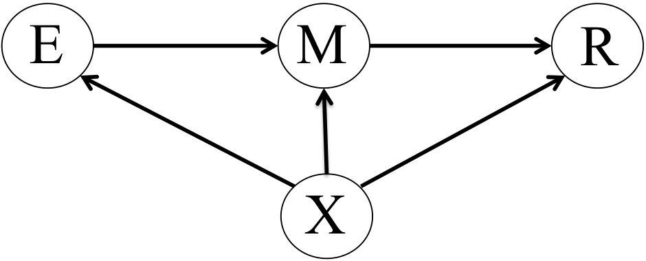 Figure 1
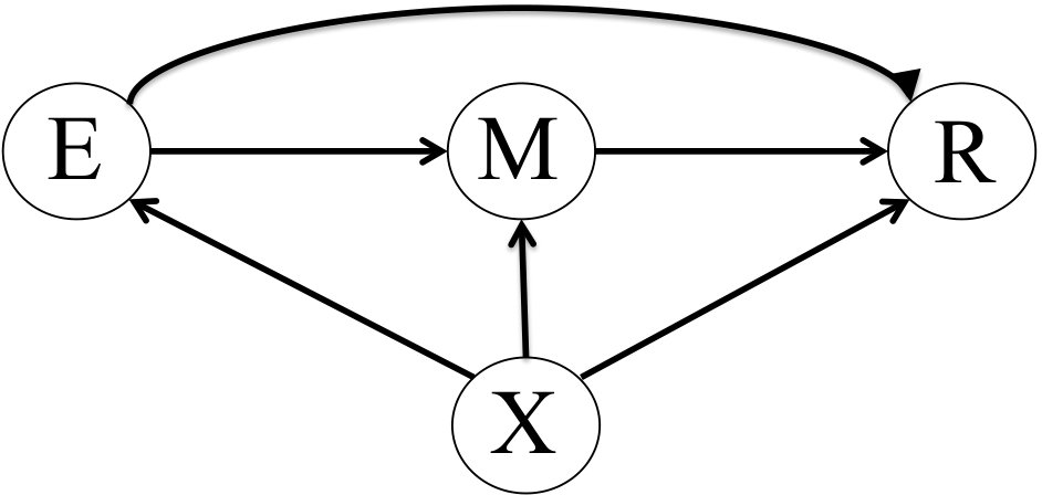 Figure 2
 Figure 3
 Figure 4
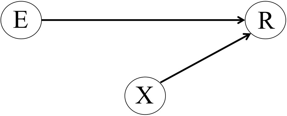 Figure 5
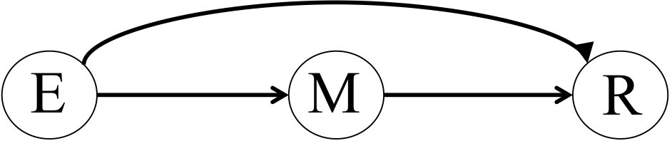 Figure 6
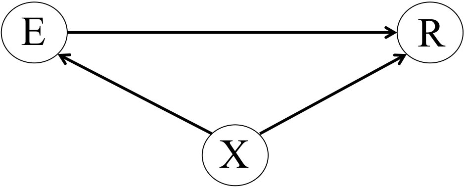 Figure 7
| Recover | Not recover | Total | |
|---|---|---|---|
| No aspirin | 12 | 88 | 100 |
| Aspirin | 30 | 70 | 100 |
| 0 | 1 | ||
| 0 | 0.70 | ||
| 1 | 0.30 | ||
| 0.88 | 0.12 | 1 | |
Peer Reviews
No public reviews on file for this paper yet. If you reviewed it on a platform where reviews are public (OpenReview, ICLR, NeurIPS, ICML), you can paste yours below so the community can read it here.
Videos
No videos yet. Explain this paper in a talk, walkthrough, or lecture? Add one.
The Probability of Causation
Philip Dawid University of Cambridge
Monica Musio University of Cagliari
Rossella Murtas University of Cagliari
(Dedicated to the memory of Stephen Elliott Fienberg
27 November 1942–14 December 2016
)
Abstract
Many legal cases require decisions about causality, responsibility or blame, and these may be based on statistical data. However, causal inferences from such data are beset by subtle conceptual and practical difficulties, and in general it is, at best, possible to identify the “probability of causation” as lying between certain empirically informed limits. These limits can be refined and improved if we can obtain additional information, from statistical or scientific data, relating to the internal workings of the causal processes. In this paper we review and extend recent work in this area, where additional information may be available on covariate and/or mediating variables.
Key words: Balance of probabilities, Causes of effects, Counterfactual, Group to individual inference, Mediator, Potential response, Sufficient covariate
1 Introduction
Many legal proceedings hinge on the assignment of blame or responsibility for some undesirable outcome. In a civil case a patient may sue a pharmaceutical company for damage caused as a side effect of one of its products; or a state health department may bring an action against a tobacco company for not disclosing information it had on the health risks of smoking, thus (it is claimed) leading to unnecessary deaths.
In many such cases there will be no dispute about the facts at issue. The patient took the drug and suffered the side effect. The tobacco company admits to having withheld the information. What remains at issue is the causal relation between the established facts. But any attempt to understand this quickly throws us into the philosophical quagmire of counterfactual reasoning, where we have to consider what might have happened in circumstances known to be false. Whether or not the patient’s suit succeeds will depend on whether or not she can prove, to the appropriate legal standard (e.g., “on the balance of probabilities”) that she would not have developed the same outcome, had she not taken the pharmaceutical product. The damages that the tobacco company are liable for will depend on an assessment of how many lives could have been saved, had they made the information available.
In this article we concentrate on cases of the first kind, where it is desired to assess whether or not the same outcome would have occurred had the putative causal event been absent. Typically, epidemiological evidence will be admitted as to the frequency of the adverse outcome, both in patients who have, and in patients who have not, been exposed to the product. Although such evidence is clearly of relevance, it is less clear exactly how. A common procedure is to compute the relative risk (RR), obtained by dividing the frequency of the outcome among those exposed to the product by the corresponding frequency among those not so exposed. And it is frequently asserted that a relative risk exceeding 2 is enough to prove that the “probability of causation” (PC) exceeds 0.5, and thus to establish a causal link “on the balance of probabilities”.
In this paper we consider such arguments in greater detail. We explain why it is difficult to establish a precise value for the probability of causation on the basis of epidemiological or other scientific evidence, which at best can only provide interval bounds for PC. We also show how it is possible to reduce the uncertainty about PC by collecting and taking account of additional data, so shedding some light on the internal workings of the causal black box.
The work presented here builds on a long-standing interaction and collaboration with Stephen Fienberg, as represented in particular by the recent papers [Dawid et al. (2014), Dawid et al. (2015), Dawid et al. (2016b)]. This formed a very small component part of Steve’s many highly significant contributions to the correct use of Statistics in the Law, which work, substantial as it was, itself constituted only a very small component of his numerous original and highly influential contributions over an enormous range of statistical topics. He was a delightful friend and a stimulating colleague and companion; he is sorely missed.
2 Group to individual analysis: The basic problem
Epidemiology attempts to discover causal relationships, such as between a certain exposure, and a certain response, . Such a relationship can be intuitively represented by a diagram such as that of Figure 1. (There is a formal semantics underlying such diagrams, but we shall not delve into that here).
Epidemiological experts are frequently called on to testify in cases revolving around the assignment of individual responsibility. However, such testimony can only concern the behaviour of groups of individuals, and its relevance to any individual case is at best indirect. The general issue of “group-to-individual” (“G2i”) inference has recently become a centre of attention both within and outside the Law [Faigman et al. (2014)].
In our context, the important distinction to be made is between inference about “Effects of Causes” (“EoC”), and inference about “Causes of Effects” (“CoE”). The former, concerning the likely outcome of a contemplated intervention or exposure, in a specific or generic individual, is the focus of most scientific investigation and experimentation, including epidemiological studies. However, it is the latter, concerning the possible causes of an observed effect in an individual case, that is of most relevance for the Law. The distinction between EoC and CoE is crucial, but all too often goes unremarked and unappreciated.
We illustrate the subtle relationship between these two forms of inference by means of an example [Dawid (2011), Dawid et al. (2014)].
Effects of Causes (EoC)
Ann has a headache. She is wondering whether to take aspirin. Will that cause her headache to disappear?
Causes of Effects (CoE)
Ann had a headache and took aspirin. Her headache went away. Was that caused by the aspirin?
To assist in addressing these questions, we assume that we have data from a very large, well-conducted, randomised trial of the success of aspirin in curing headaches, whose subjects can be assumed to be similar to Ann in the way they respond. This yields percentages as in the following table:
3 A framework for analysis
Effects of Causes (EoC)
Ann can argue as follows “If I take the aspirin, I will be just like the subjects in the treatment group, so I can assess my probability of recovery in this case as 30%. Similarly, If I don’t take the aspirin, my probability of recovery in that case can be assessed to be 12%. Other things being equal, it would be better to take the aspirin.” While this argument does, not, perhaps address the question exactly as posed, it does give Ann fully adequate guidance to address and solve her EoC decision problem. What is at issue was the as yet unknown event of recovery, and the data are directly relevant for assessing uncertainty about that unknown outcome (for each of the two decisions that Ann might take).
Causes of Effects (CoE)
Things are very different for the CoE question. Indeed, there is now no unknown event: We know that Ann definitely took the aspirin, and she definitely recovered. What is at issue here is not uncertainty about an as yet unknown event, but uncertainty about a relationship between known events: the existence, or otherwise, of a causal relationship between taking the aspirin and recovering.
3.1 Counterfactuals and potential outcomes
One way of thinking about whether a certain outcome was caused by a certain exposure is to ask the question: “Would the same outcome still have occurred, even if the exposure had been absent?”. Because this question is posited on a hypothesis that is known to be false, and thus counter to known facts, it is termed a counterfactual query. There is much discussion of counterfactuals in the philosophical literature (see e.g. [Menzies (2014)]), and they raise many perplexing problems. In particular, is it even meaningful to regard a counterfactual as having a definite (even if unknown) truth value?
Supposing that we can talk of the truth value of counterfactual, we might reinterpret the assertion “The exposure caused the outcome” as:
“Both the exposure and the outcome occurred; and had (counterfactually) the exposure not occurred, neither would the outcome have occurred.”
With this interpretation, and taking account of the known facts, the truth value of the assertion “The exposure caused the outcome” becomes identified with the (typically unknown) truth value of the counterfactual proposition “In the counterfactual world where the exposure did not occur, the outcome did not occur”.
Some comments
- (i).
There is an implicit “ceteris paribus” condition in the above interpretation. In the counterfactual world being considered, we are changing the truth value of the exposure, but nothing else—or, at any rate, nothing else occurring before, or simultaneously with, the exposure. We must of course allow for the outcome to change, and we might possibly also allow changes to other, later, events (perhaps intermediate between the exposure and the outcome), in the light of the change to the exposure. Since there are various ways in which our counterfactual comparison world can be constructed, there is a resultant ambiguity in the truth value of the counterfactual assertion. [Lewis (1973)] argues that we should use the “closest possible world” to the real world, subject to the counterfactual change in the exposure—but this still leaves a great element of vagueness. 2. (ii).
There may be some choice as to what the counterfactual value of the exposure would have been, if it had been other than it actually was. If Ann had not taken two aspirins, she might have taken none at all, or taken three aspirins, or taken two paracetamol tablets, or gone to bed with a wet towel around her head. The counterfactual query only becomes precise when we have fully specified the “counterfactual foil” for comparison with the factual exposure. 3. (iii).
There will typically be a variety of different exposures that we can consider. For example, Ted has been a smoker for 20 years, has lived by a busy main road which is subject to high air pollution, and has developed lung cancer. Then we could ask “Was Ted’s cancer caused by his smoking?”, “Was it caused by his air pollution exposure?”, “Was it caused by his smoking and the air pollution jointly?”, etc., etc. Each of these questions involves consideration of a different counterfactual world for comparison with the real world, and there is no reason why we could not regard all of them as true simultaneously—which leads to some difficulties in understanding what might be the “actual cause” of Ted’s cancer (see [Halpern (2016)] for a thoughtful analysis of the elusive concept of “actual cause”). In particular, we should not express “Ted’s smoking caused his cancer” as “The cause of Ted’s cancer was his smoking”—though we might say “A cause of Ted’s cancer was his smoking”. The former phrasing suggests, misleadingly, that there is a variable, “The cause of Ted’s cancer”, that can take different values (e.g., smoking, air pollution, natural causes). But as these putatuve causes are not mutually exclusive, there can be no such variable. And when we can assign probabilities to “Ted’s smoking caused his cancer”, “Air pollution caused Ted’s cancer”, etc., it is perfectly acceptable for these to sum to more than 1. (For a specific example of this, see [Hutchinson et al. (1991)]).
The standard framework of probability theory does not easily admit argument about counterfactual worlds and uncertain relationships. To formulate such questions meaningfully, we need to expand the universe of discourse. The way this has traditionally been done in statistics is by the introduction of so-called “potential outcomes” [Neyman (1935), Rubin (1978)]. We consider a binary exposure, or cause, variable , and a binary response, outcome, or effect, variable . For each value or of , we introduce a variable , conceived as the value that would assume, were it the case that . If in the actual world (say), then the observed outcome will be ; in this case we have no way of observing , which thus becomes a (necessarily unobservable) counterfactual variable. Similarly, if in the actual world , then , and becomes counterfactual and unobservable. It is typically assumed, explicitly or implicitly, that the bivariate variable {\mbox{\mathbf{R}}}:=(R_{0},R_{1}) is determined before the value of is, and does not depend on how that value of came to be determined or known (for example, whether by external intervention, or by observation alone). The effect of setting or observing (say) is just to uncover the pre-existing value of , and identify with . In particular, although the pair is modelled probabilistically just like any other bivariate random variable, there is the epistemic problem that there are no circumstances in which it would be possible to observe both its constituent values. This has been termed “the fundamental problem of statistical causality” [Holland (1986)].
The framing and analysis of causal questions in terms of potential outcomes has become the industry standard in statistical causality. For the investigation of “effects of causes”’, it has been strongly argued that this approach is both unnecessary and potentially misleading [Dawid (2000), Dawid (2015)]. However, for studying causes of effects there is currently no alternative to the use of potential outcomes to model counterfactual possibilities. Nevertheless, the logical difficulty that the bivariate quantity can never be fully observed creates subtle problems that must not be ignored.
3.2 The probability of causation
Armed with the above machinery and notation, we can now formulate an expression for the probability of causation.
We interpret the expression “the exposure causes the outcome ” as the event “EC: ”. This encodes the property that the potential response to is , while at the same time the potential response to is [math]. However, although we have thus expressed the causality relation as an event, in what appears to be a standard probabilistic framework, the fundamental problem of statistical causality implies that this is an event whose truth value can never be determined.
Suppose now that (for Ann) we have observed and (or, equivalently, and ). Since we must condition on all known facts, the appropriate expression for the probability of causation (in Ann’s case) is
[TABLE]
However, merely establishing a notational expression for the probability of causation does not, of itself, solve the problem of how to evaluate this quantity, involving as it does the probability of an unobservable event.
The approach we shall take is to regard the pair as having a joint distribution (jointly with all other variables in the problem), but to make no assumptions about that distribution, other than any constraints imposed by empirically observable information. Typically it will not then be possible to identify that joint distribution fully, but only to constrain it within limits—though those limits will depend on the precise form of the available information.
There is a further point that needs to be taken into account. The variables in (1) are those pertaining specifically to Ann, and the joint distribution Pr appearing in it is thus a distribution over those specific variables. But who is the analyst assigning this distribution? It might be Ann herself, or some onlooker. These individuals will typically have different background information, and so different distributions. In particular, an onlooker might reasonably infer, merely from observing that Ann decided to take the aspirin (, that her headache is particularly bad, and consequently that her potential responses and are both likely to be poorer than if he did not have this information. For Ann, however, the severity of her headache is known background information that is already taken into account in her own distribution, and the mere fact that she is contemplating taking the aspirin gives her no additional information about her potential responses. That is to say, for Ann’s own probability distribution we can reasonably invoke the “no confounding” assumption,
[TABLE]
which expresses probabilistic independence between the fact of her exposure, . and the pair of her potential responses. In this case expression (1) simplifies to
[TABLE]
However, for the onlooker who is not initially aware of the severity of Ann’s headache, it may be inappropriate to accept (2), and hence (3).
In most of the sequel (with the exception of § 5) we shall assume that the analyst has sufficient background information about Ann for (2) to be true (to a good enough approximation), and hence use (3) as the expression for the probability of causation. Furthermore, because we shall wish to use external data from other individuals to assist in estimating the analyst’s probability distribution Pr for Ann, we shall also need to assume that the background information the analyst has on those individuals is essentially the same as what he111We refer to the analyst in the masculine, to distinguish him from the subject, Ann—while not precluding that they could be the same individual. has for Ann — a condition that can sometimes be met by restricting the set of external individuals considered. Even so, these assumptions, necessary for much of our analysis, are highly restrictive, and will often be inappropriate. Careful consideration must be given to their suitability before applying our results.
4 Basic analysis
We start by considering the case that the only available empirical information is that presented in Table 1.
Assuming the analyst can regard the individuals in the trial as similar to Ann, he might argue: “When Ann takes aspirin, she puts herself in the same position as those external individuals in the treatment group, of which recovered. Because of the no confounding assumptions (both in the data and for Ann), this means that her potential response to taking aspirin, , has a 30% probability of taking the value (Recover). I can thus identify my marginal probability (for Ann), . Similarly, I can evaluate my marginal probability . However, because of the fundamental problem of statistical causality, there is no further empirical information available relating to my joint distribution of .”
Armed with this limited information, the analyst can attempt to fill in the entries in Table 2, specifying his bivariate probability distribution for . The margins are fully determined by the above empirically informed probabilities, but since he has no empirical information directly relevant to the joint probability , he simply enters an unknown (and unknowable) value in the associated internal cell of the table. In combination with the known marginal probabilities, this allows completion of the body of the table, as shown.
Now although the precise value of remains unknown, from the table we can extract partial information about it, using the fact that any probability must be nonnegative. Applying this principle to the four entries in the body of the table, we obtain: , , , . Combining these and omitting redundancies gives the inequality: . This interval bound is the full information available about on the basis of the empirical data.
Now because of assumption (2), . Thus the analyst can assert:
[TABLE]
Even under the restrictive assumptions that have been made, this wide interval bound is all that can be deduced, from the empirical data, about the probability of causation in this particular case.
The above logic can be applied in the general case, leading to the following interval bound in terms of empirically estimable quantities (under our no-confounding assumptions):
[TABLE]
where
[TABLE]
is the (causal) risk ratio. We note that implies , which might be taken to prove causation “on the balance of prbabilities”. However, if we can not deduce from (5) that (to reject causation, on the balance of probabilities).
5 Allowing for unobserved confounding
When we cannot assume (2) we cannot simply apply the above theory directly, since the very fact that Ann decided to take the aspirin gives the analyst some indirect information about Ann’s state of health—in the light of which it would no longer be appropriate to consider her as similar to the individuals in the experimental study, for which this information was not available. [Tian and Pearl (2000)] showed that in this situation we can still obtain bounds for PC, so long as, in addition to the experimental data, we also have observational data on individuals whose behaviour (in the opinion of the analyst) can be considered similar to that of Ann, in that they have the same dependence as she does between their decision to take the aspirin and their pair of potential responses. [Tian and Pearl (2000)] then derive the following interval bounds:
[TABLE]
where denotes the recovery probability in the experimental control group, who were externally assigned to have set to [math]; while the other probabilities are obtained from the observational data (interestingly, we do not require experimental data on those who were assigned treatment).
For example, suppose that, in addition to the experimental data of Table 1, we have observational data in which . We then find that the lower bound in (7) is —allowing us to establish causation with certainty.
6 Peeking into the box
So far we have considered the relationship between exposure and response as a causal “black box”, without attempting to understand or model its hidden mechanisms in any further detail. If we are willing to make some assumptions about these mechanisms, or access external information about them, we can make better causal inferences from our data—even in the absence of any further information about Ann.
6.1 Monotonicity and beyond
One assumption commonly made is monotonicity. In a context such as ours, this would say that, if recovery would have occurred without the treatment, it would certainly occur with the treatment. That is to say, . This implies in particular , or equivalently . This is a constraint on the margins of a table such as Table 1, and so could be falsified; but even when this marginal constraint is satisfied, there is typically no further information to help us decide whether monotonicity holds or not. Nevertheless it is frequently taken as a reasonable requirement, and would add one further constraint on the entries in Table 1: . Since in that table , we can then compute the exact value , so that . Here (as in general), monotonicity allows as to replace the interval given by (5) by its lower endpoint . In this case, does imply .
Monitonicity, while appealing, is a strong, perhaps overstrong, assumption about the internal workings of the causal black box. Moreover, because it is a property of the pair of values considered jointly, the fundamental problem of statistical causality implies that we can never expect to obtain empirical evidence to let us decide whether or not monitonicity does in fact hold. For that reason we take a different approach in the rest of this paper, focusing on using additional, empirically observable, information to shed some light on internal causal mechanisms, and thus improve causal inferences. In such cases, although we typically cannot obtain an exact point value for the probability of causation, we may be able to narrow the interval bounds on it. We shall particularly consider cases in which we might have information on additional covariates and/or mediators that influence the causal pathway.
7 Covariate information
Suppose that, in the experimental data, we can also observe an additional covariate, — an individual characteristic that can vary from person to person, and can affect that person’s response. This situation is represented by the diagram of Figure 2.
For simplicity, we suppose that can only take a discrete set of values. We can then estimate, from the data, the response probability, , among those individuals having covariate value and exposure level ( or ).
In those cases that we are also able to measure for Ann, say , we can simply restrict the experimental subjects to those having the same covariate value (who are thus like Ann in all relevant respects), and apply the analysis of § 4. We can then use formula (5), after first replacing all the probabilities in (5) and (6) by their conditional versions, given .
However, it turns out that we can make use of the additional covariate information in the experimental data, even when we cannot observe for Ann. For this case, it is shown in [Dawid (2011)] that we have the interval bounds
[TABLE]
where
[TABLE]
and that this interval is always contained in that given by (5), which ignores the additional covariate information.
Example 7.1
Suppose that the covariate is binary, taking values [math] and with equal probability. Suppose further that, from the experimental data, we obtain the following probabilities:
[TABLE]
These imply marginal recovery probabilities (not taking the value of into account):
[TABLE]
- (i).
If we had not observed , either in the data or in Ann, we would use the marginal values, to obtain a relative risk of , and interval bounds
[TABLE] 2. (ii).
If we observe both in the data and in Ann, we obtain
[TABLE]
if Ann has , and
[TABLE]
if Ann has . 3. (iii).
Finally, if we have observed in the data but not in Ann, the relevant interval becomes
[TABLE]
an improvement on that of (i)
8 Sufficient covariate
In § 7 above it was assumed that the assignment of exposure was unrelated to the covariate . Here we relax this, and allow to influence both the exposure and the response . But we assume that there are no further, unobserved, variables that might act to confound this relationship— is a “sufficient covariate” [Guo and Dawid (2010), Dawid (2015)] for assessing the causal effect of on . The relevant diagram is now that of Figure 3.
We assume that the identical same structure holds for the individuals in the data and for Ann. is observed in the data, but possibly not for Ann.
When is observed for Ann, say , we can again apply the basic inequalities (5), after replacing the probabilities in (5) and (6) by their conditional versions, given .
When is not observed for Ann, the interval bounds for PC become:
[TABLE]
Now in this case we can alternatively use the “back-door formula” [Pearl (2009)]:
[TABLE]
to recreate the experimental response rate among the controls—and so compute the interval (7). However, this would be tantamount to ignoring the additional information on in the data. It can be shown that the interval given by (9) is always contained in that given by (7).
Example 8.1
Suppose is binary, and from the data we obtain the following probabilities:
[TABLE]
Then we obtain the following lower bounds for the probability of causation (the upper bound being 1 in all cases):
[TABLE]
9 Complete mediator
We now turn to consider the case, represented by the diagram in Figure 4, that the causal effect of on is completely mediated by some variable , assumed for simplicity to be binary. That is to say, affects and effects , and the combination of these two pathways constitutes the totality of the effect of on .
We assume that there is no further confounding of either of these relationships, either in the data or for Ann. We shall consider the case that all three variables are observed in the data, but that we only observe and for Ann.
Note that our assumptions imply the conditional independence property R\,\mbox{\perp!!!\perp}\,E\,|\,M, so that
[TABLE]
which should hold, at least approximately, in the data. In any event, we should estimate using formula (11), rather than directly. (We could also have separate experimental data on the and relationships, and apply (11).)
It is shown in [Dawid et al. (2016a)] that (with this understanding) the additional information on the mediator does not affect the lower bound in (5). However, we obtain the following improved upper bound:
[TABLE]
Example 9.1
Suppose we obtain the following values from the data:
[TABLE]
Marginalising over using (11), we obtain the same values as in Table 1. On applying (12), we get ; whereas without taking account of the mediator the bounds were .
We can elaborate the above analysis by allowing for an additional sufficient covariate , as represented by Figure 5, that can modify all the above marginal and conditional probabilities, and conditional on which is a complete mediator.
We assume that is always observed in the data. If we observe for Ann, we simply replace all probabilities by their versions further conditioned on , yielding bounds , say. If we do not observe in Ann, the lower bound is , and the upper bound is .
10 Partial mediator
In the case of a partial mediator, as represented by Figure 6, there us an additional “direct effect” of on , that is not mediated by (again supposed binary, for simplicity). So now we have to consider the effect of on , and the joint effect of and on . Again we suppose that there is no further confounding of these relationships, either in the data or for Ann, and consider the case that all three variables are observed in the data, but that we only observe and for Ann.
In [Murtas et al. (2016)] it is shown that, once again, the lower bound for PC is unaffected by the additional information on . However, we are able to abtain a new upper bound , where
[TABLE]
Example 10.1
Suppose that, from the data, we estimate the following probabilities:
[TABLE]
Marginalising over , these imply
[TABLE]
We then obtain when accounting for the mediator, compared with when ignoring it.
However, accounting for a partial mediator may not always yield improved bounds.
Example 10.2
Suppose the probabilities estimated from the data are as follows:
[TABLE]
These imply
[TABLE]
The lower bound is . The upper bound obtained from (13) is . However, just ignoring , and applying (5), we get upper bound , which should theregore be used in preference.
Again, we can elaborate the problem by including a sufficient covariate , conditional on which we have the above structure, as represented by Figure 7. Let the appropriate lower and upper bounds, computed with all probabilities conditioned on , be and . Then in the absence of information about for Ann, the relevant lower and upper bounds for PC are , .
11 Discussion
We have assumed throughout that the available data are sufficiently extensive to allow essentially perfect estimates of the required probabilities. Of course this will never be the case. [Dawid et al. (2016b)] consider how to make suitable inferences about PC from limited data, using a Bayesian approach.
We have presented some simple cases, involving covariates and mediators, where having additional information about the internal structure of the causal link between exposure and response enables us to refine our causal inferences. Other problems might involve a more complex collection of variables and pathways, perhaps expressed as a directed acyclic graph. It should be possible to extend our analysis to such more general cases. Information on different causal subsystems might be obtained from a variety of scientific investigations. But caution must be exercised in justifying the transfer of such information from generic scientific data to the individual case. Additional uncertainty over the correct representation of the problem must also be taken into account.
To return, finally, to the issue facing a court of law that has to return a decision on causality: we hope we have shown that this is not a simple matter! We can only express our sympathy with a judge who has to make such a decision, on the “balance of probabilities,” when the best possible conclusion, based on available scientific evidence and the kind of analysis we have presented here, is that the probability of causation lies between and .
The reference list from the paper itself. Each links out to its DOI / PubMed record.
- 1Dawid (2000) Dawid, A. P. (2000). Causal inference without counterfactuals (with Discussion). Journal of the American Statistical Association , 95 , 407–48.
- 2Dawid (2011) Dawid, A. P. (2011). The role of scientific and statistical evidence in assessing causality. In Perspectives on Causation , (ed. R. Goldberg), pp. 133––147. Hart Publishing, Oxford.
- 3Dawid (2015) Dawid, A. P. (2015). Statistical causality from a decision-theoretic perspective. Annual Review of Statistics and its Application , 2 , 273–303. DOI:10.1146/annurev-statistics-010814-020105 . · doi ↗
- 4Dawid et al . (2014) Dawid, A. P., Faigman, D. L., and Fienberg, S. E. (2014). Fitting science into legal contexts: Assessing effects of causes or causes of effects? (with Discussion and authors’ rejoinder). Sociological Methods and Research , 43 , 359--421. DOI:10.1177/0049124113515188 . · doi ↗
- 5Dawid et al . (2015) Dawid, A. P., Faigman, D. L., and Fienberg, S. E. (2015). On the causes of effects: Response to Pearl. Sociological Methods and Research , 44 , 165--74. DOI:10.1177/0049124114562613 . · doi ↗
- 6Dawid et al . (2016 a) Dawid, A. P., Murtas, R., and Musio, M. (2016 a). Bounding the probability of causation in mediation analysis. In Topics on Methodological and Applied Statistical Inference , (ed. T. D. Battista, E. Moreno, and W. Racugno), pp. 75--84. Springer.
- 7Dawid et al . (2016 b) Dawid, A. P., Musio, M., and Fienberg, S. E. (2016 b). From statistical evidence to evidence of causality. Bayesian Analysis , 11 , 725--52.
- 8Faigman et al . (2014) Faigman, D. L., Monahan, J., and Slobogin, C. (2014). Group to individual (G 2i) inference in scientific expert testimony. University of Chicago Law Review , 81 , 417--80.