Effect of intense magnetic fields on reduced-MHD evolution in $\sqrt{s_{\rm NN}}$ = 200 GeV Au+Au collisions
Victor Roy, Shi Pu, Luciano Rezzolla, Dirk H. Rischke
TL;DR
This study explores how intense external magnetic fields influence the evolution of hot nuclear matter in heavy-ion collisions, revealing increased elliptic flow and altered momentum eccentricities depending on magnetic field dynamics.
Contribution
It introduces a model for external magnetic fields affecting 2+1D reduced-MHD evolution in Au+Au collisions, considering different electrical conductivities of the QGP.
Findings
Magnetic fields cause significant changes in momentum eccentricities.
Elliptic flow coefficient v2 increases with magnetic field presence.
Results depend on magnetic field decay and initial strength.
Abstract
We investigate the effect of large magnetic fields on the dimensional reduced-magnetohydrodynamical expansion of hot and dense nuclear matter produced in = 200 GeV Au+Au collisions. For the sake of simplicity, we consider the case where the magnetic field points in the direction perpendicular to the reaction plane. We also consider this field to be external, with energy density parametrized as a two-dimensional Gaussian. The width of the Gaussian along the directions orthogonal to the beam axis varies with the centrality of the collision. The dependence of the magnetic field on proper time () for the case of zero electrical conductivity of the QGP is parametrized following [Deng 2012], and for finite electrical conductivity following [Tuchin 2013]. We solve the equations of motion of ideal hydrodynamics for such an external magnetic field. For collisions…
Click any figure to enlarge with its caption.
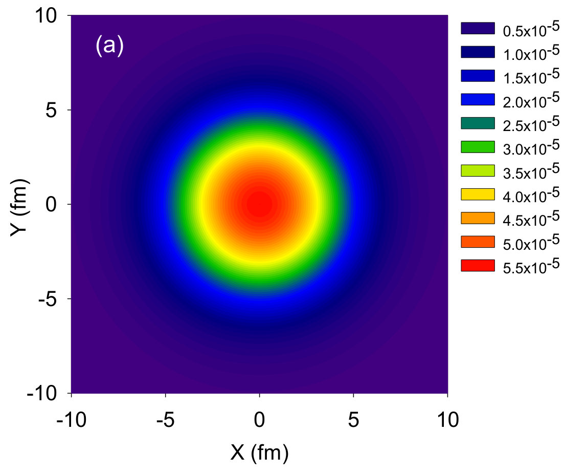 Figure 1
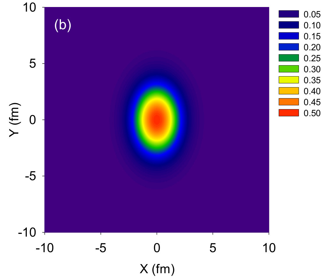 Figure 2
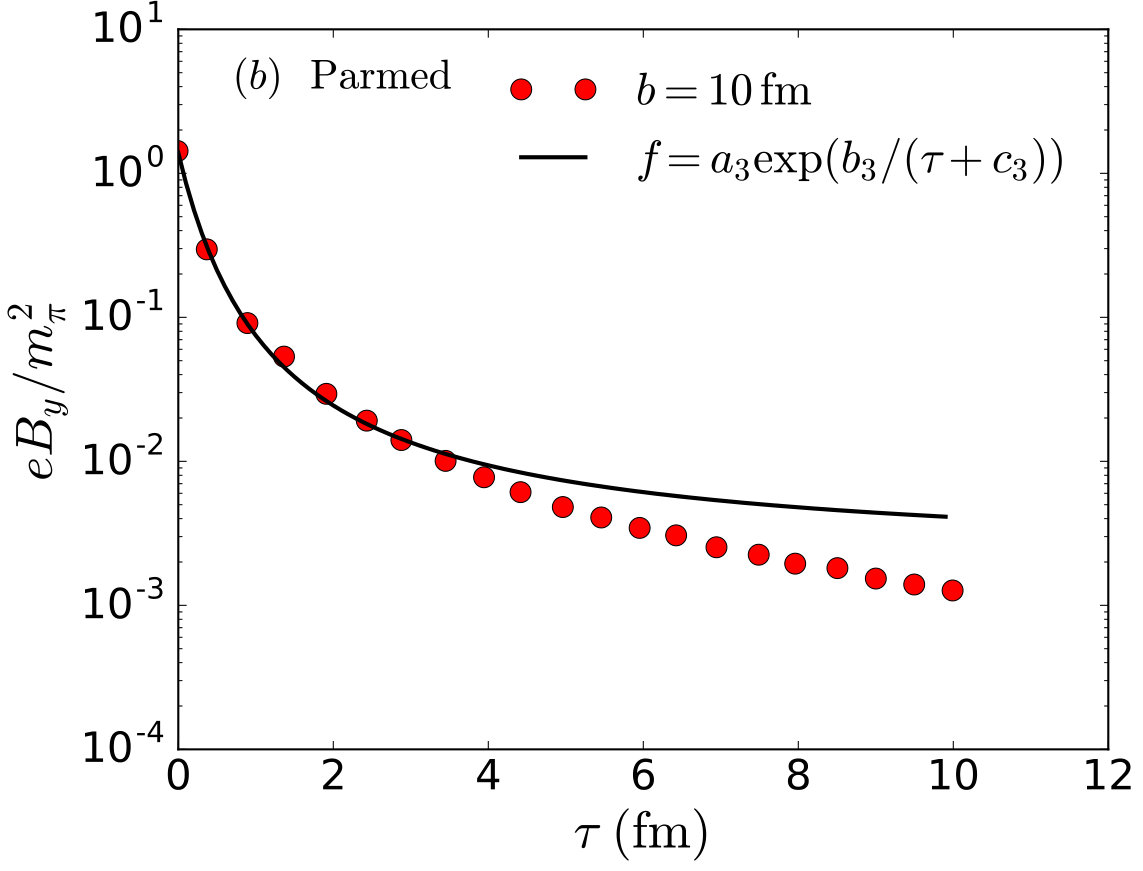 Figure 3
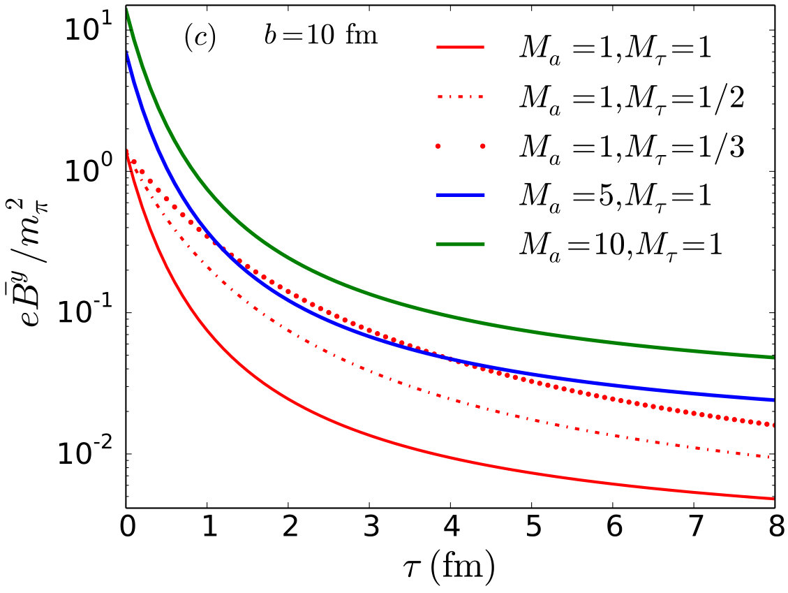 Figure 4
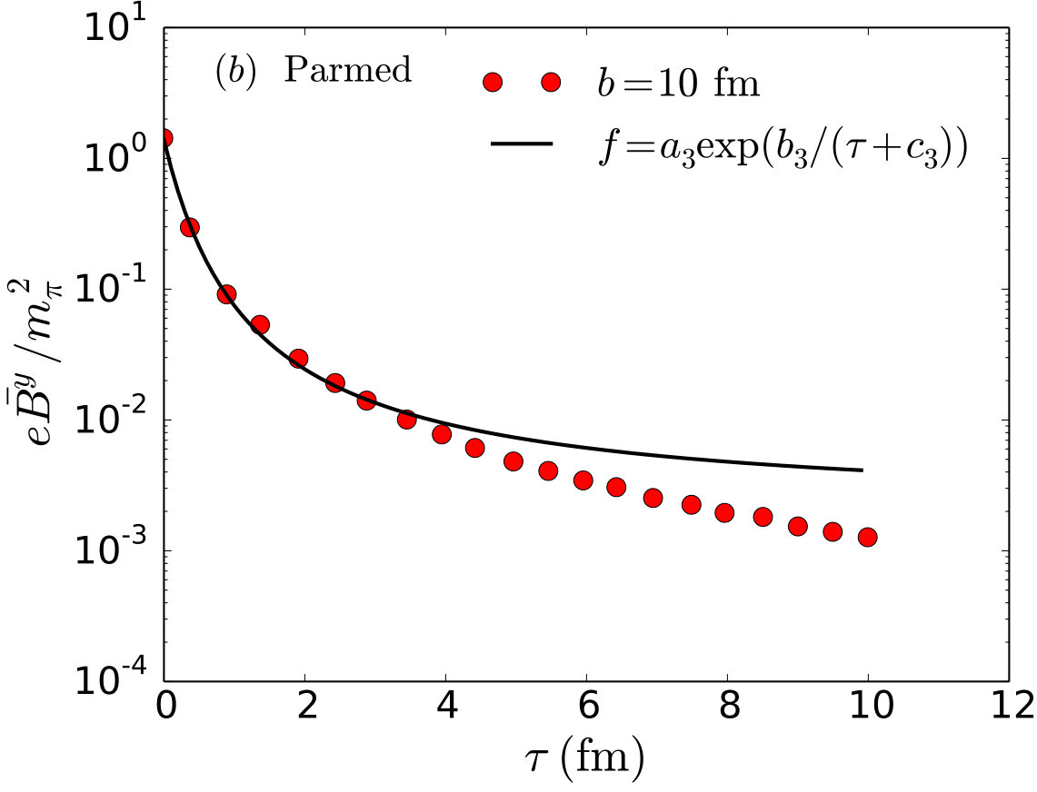 Figure 5
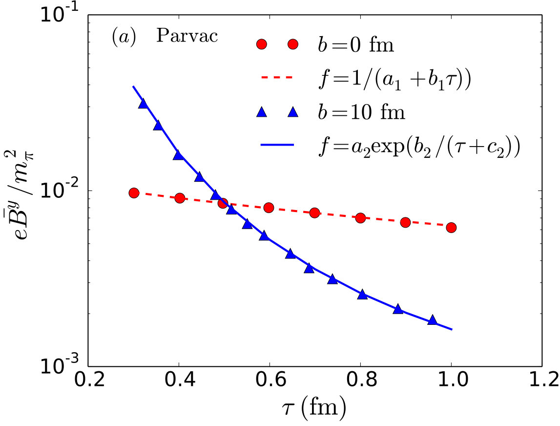 Figure 6
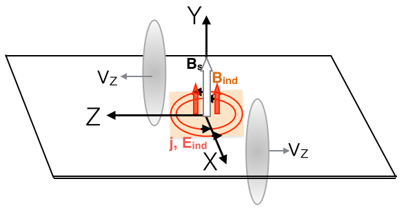 Figure 7
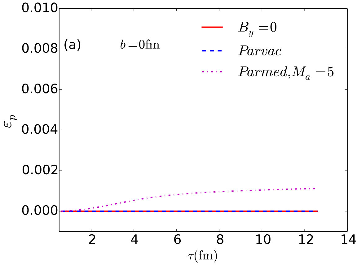 Figure 8
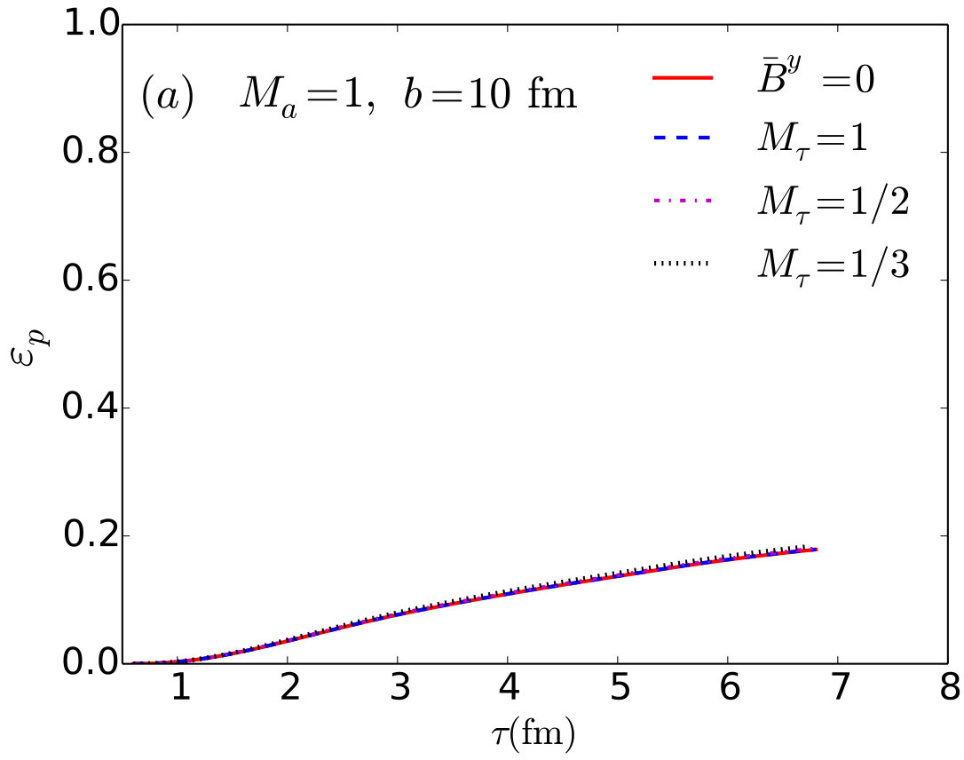 Figure 9
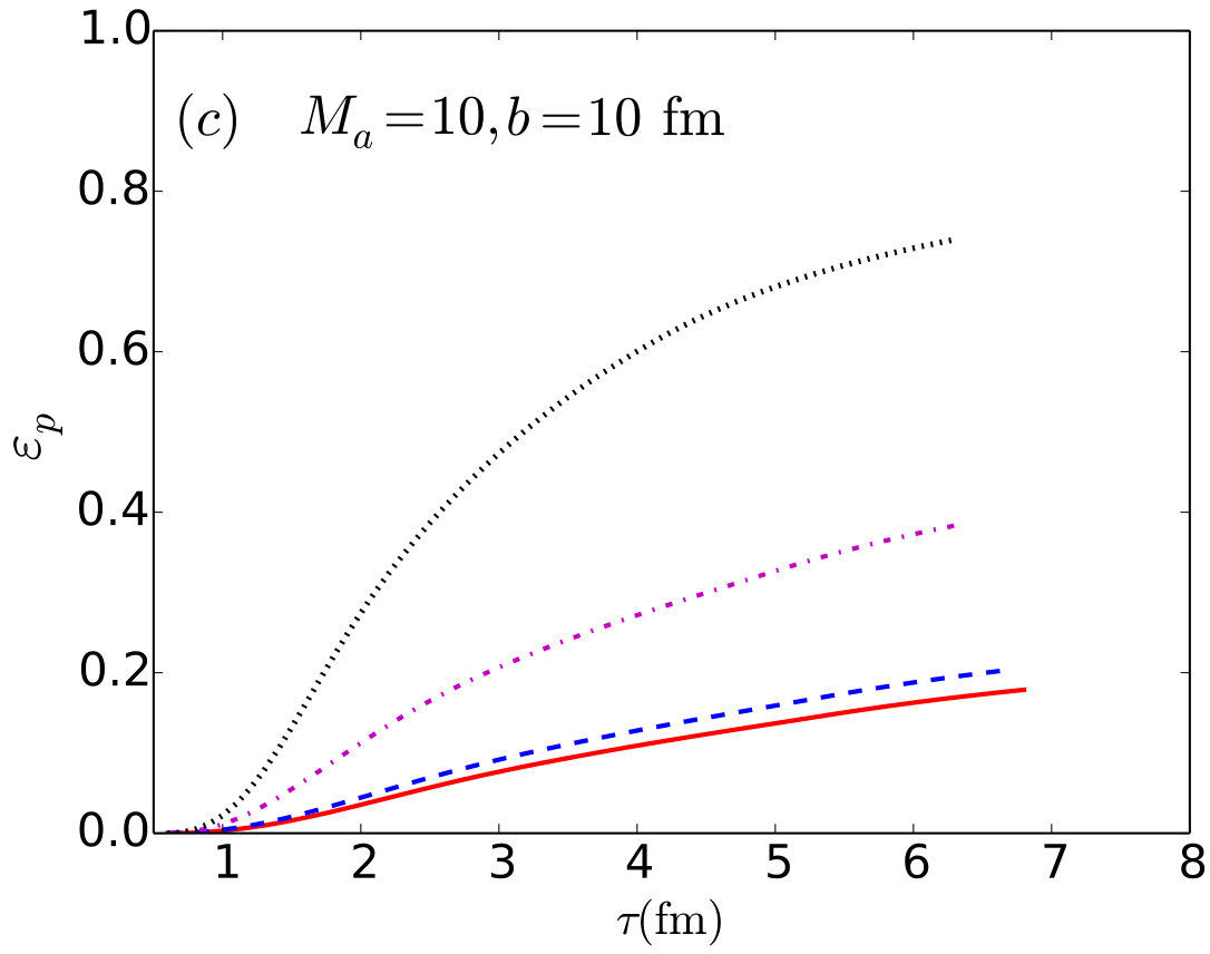 Figure 10
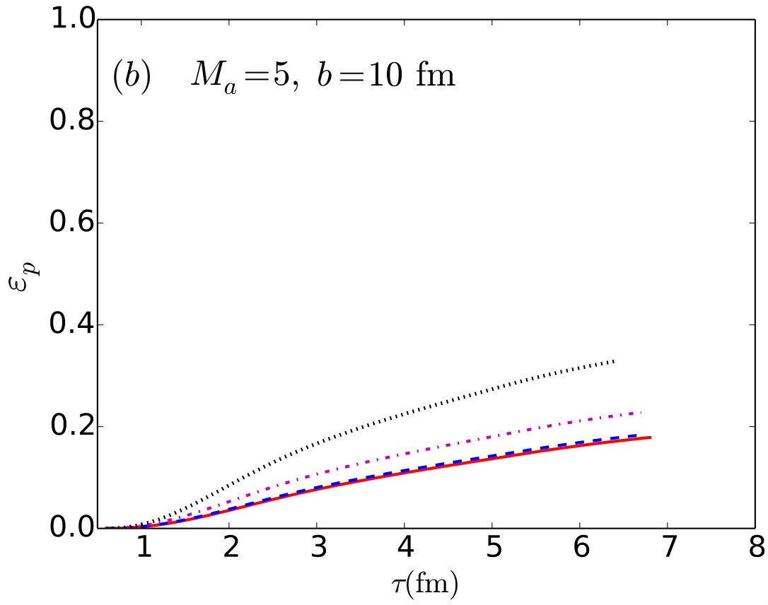 Figure 11
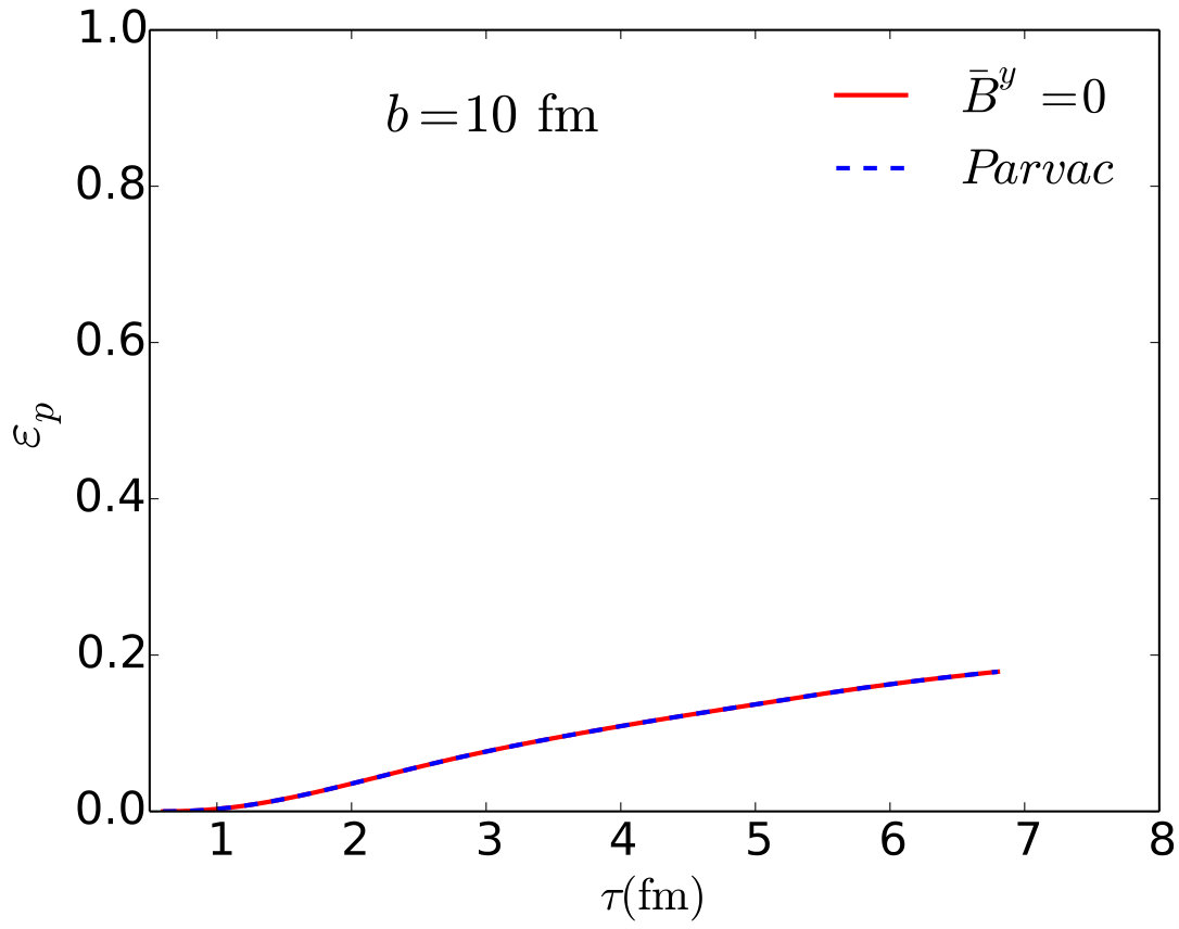 Figure 12
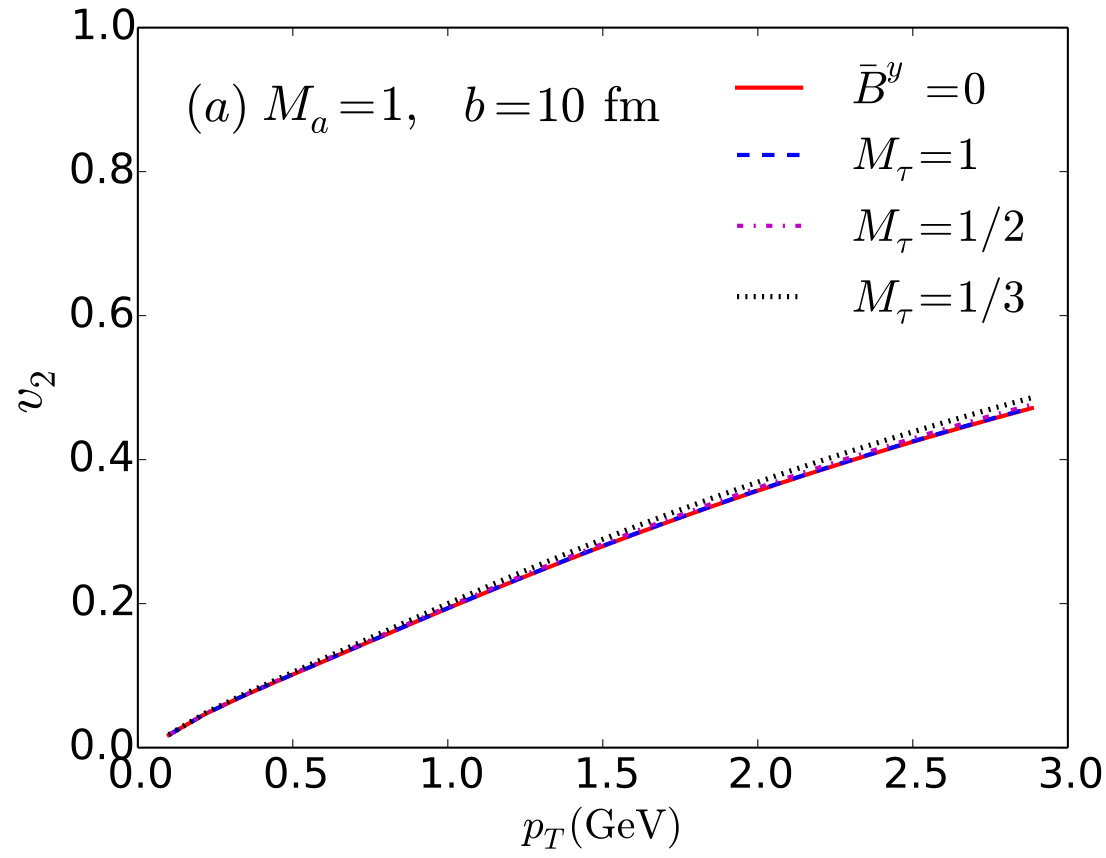 Figure 13
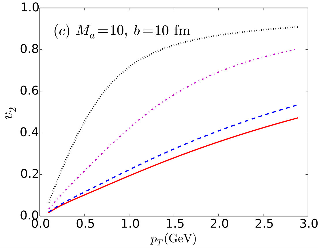 Figure 14
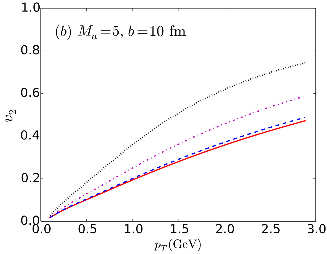 Figure 15
Peer Reviews
No public reviews on file for this paper yet. If you reviewed it on a platform where reviews are public (OpenReview, ICLR, NeurIPS, ICML), you can paste yours below so the community can read it here.
Videos
No videos yet. Explain this paper in a talk, walkthrough, or lecture? Add one.
Effect of intense magnetic fields on reduced-MHD evolution in
= 200 GeV Au+Au collisions
Victor Roy1, Shi Pu2, Luciano Rezzolla3,4, Dirk H. Rischke3,5
1National Institute of Science Education and Research, HBNI, 752050 Odisha, India.
2Department of Physics, The University of Tokyo, 7-3-1 Hongo, Bunkyo-ku, Tokyo 113-0033, Japan
3Institute for Theoretical Physics, Goethe University, Max-von-Laue-Str. 1, D-60438 Frankfurt am Main, Germany
4Frankfurt Institute for Advanced Studies, Ruth-Moufang-Str. 1, D-60438 Frankfurt am Main, Germany
5Department of Modern Physics, University of Science and Technology of China, Hefei, Anhui 230026, China
Abstract
We investigate the effect of large magnetic fields on the dimensional reduced-magnetohydrodynamical expansion of hot and dense nuclear matter produced in = 200 GeV Au+Au collisions. For the sake of simplicity, we consider the case where the magnetic field points in the direction perpendicular to the reaction plane. We also consider this field to be external, with energy density parametrized as a two-dimensional Gaussian. The width of the Gaussian along the directions orthogonal to the beam axis varies with the centrality of the collision. The dependence of the magnetic field on proper time () for the case of zero electrical conductivity of the QGP is parametrized following Ref. Deng:2012pc , and for finite electrical conductivity following Ref. Tuchin:2013apa . We solve the equations of motion of ideal hydrodynamics for such an external magnetic field. For collisions with non-zero impact parameter we observe considerable changes in the evolution of the momentum eccentricities of the fireball when comparing the case when the magnetic field decays in a conducting QGP medium and when no magnetic field is present. The elliptic-flow coefficient of is shown to increase in the presence of an external magnetic field and the increment in is found to depend on the evolution and the initial magnitude of the magnetic field.
I Introduction
Two positively charged heavy nuclei produce ultra-intense magnetic fields in collider experiments at the Relativistic Heavy Ion Collider (RHIC) and at the Large Hadron Collider (LHC), e.g. for 200 GeV Au+Au collisions. The intensity of the magnetic field in the transverse plane grows approximately linearly with the center-of-mass energy () Bzdak:2011yy ; Deng:2012pc ; Tuchin:2013apa [see also recent studies including non-zero chiral conductivity Tuchin:2014iua ; Li:2016tel ]. The corresponding electric field in the transverse plane also becomes very large since it is enhanced by a Lorentz factor. Such intense electric and magnetic fields are believed to have a strong impact on the dynamics of high-energy heavy-ion collisions. For example, a strong magnetic field may induce energy loss of fast quarks and charged leptons via synchrotron radiation Tuchin:2010vs , or may enhance dilepton and photon production Tuchin:2010gx ; Basar:2012bp . There are several other interesting phenomena related to the presence of ultra-intense magnetic fields in heavy-ion collisions. For example, in the case of an imbalance in the number of left- vs. right-handed fermions, a charge current is induced in the Quark-Gluon Plasma (QGP), leading to the separation of electrical charges, which is known as the “chiral magnetic effect” (CME) Kharzeev:2007jp . Within a 3+1 dimensional anomalous hydrodynamics calculation, Ref. Hirono:2014oda showed that the CME could be seen in azimuthal correlations of charged hadrons. Along with the CME, it was also theoretically predicted that massless fermions with the same charge but different chirality will be separated, known as “chiral separation effect” (CSE). A connection between these effects and the Berry phase in condensed-matter systems was pointed out in Refs. Son:2012wh ; Son:2012zy ; Stephanov:2012ki ; Gao:2012ix ; Chen:2012ca ; Hidaka:2016yjf , and some nonlinear chiral transport phenomena were studied in Refs. Pu:2014fva ; Chen:2016xtg ; Ebihara:2017suq ; Gorbar:2016qfh . Within the statistical hadron-resonance gas model of Ref. Bhattacharyya:2015pra , significant changes of hadron multiplicities were observed in the presence of a strong magnetic field. Finally, the possibility of a change in the quark-hadron phase transition line in the QCD phase diagram under the combined influence of external magnetic field and local vortices was explored in Ref. McInnes:2016dwk ; we refer the reader to the recent reviews Kharzeev:2013ffa ; Bzdak:2012ia ; Kharzeev:2015kna ; Tuchin:2013ie ; Huang:2015oca , where more details can be found.
Relativistic dissipative hydrodynamics has so far been successfully applied to explain the experimentally measured flow harmonics in heavy-ion collisions. The success of hydrodynamics implies that a QGP with small shear-viscosity to entropy-density ratio is formed in Au+Au collisions at top RHIC energies within a short time interval Shen:2011zc ; Romatschke ; Heinz ; Bozek:2012qs ; Roy:2012jb ; Heinz:2011kt ; Niemi:2012ry ; Schenke:2011bn . The system is close to local equilibrium, thus the initial geometry of the collision has a strong influence on the final momentum anisotropy. However, the possible effect of a magnetic field on the hydrodynamical evolution has so far not been studied extensively, except for some simplified cases Gursoy:2014aka ; Zakharov:2014dia and most recently using some approximate form of the equations of relativistic magnetohydrodynamics (MHD) Pang:2016yuh ; Das:2017qfi , or employing a 3+1-dimensional partonic cascade BAMPS (Boltzmann Approach to Multi-Parton Scatterings) Greif2017 .
In a parallel analytical approach, in Refs. Roy:2015kma ; Pu:2016ayh ; Pu:2016bxy solutions of the ideal-MHD equations were found in simplified geometries. More specifically, for Au+Au collisions at 200 GeV, the electromagnetic field energy was shown to be comparable to the initial energy density of the QGP in Ref. Roy:2015coa . In a recent work Mohapatra:2011ku , it was argued that a magnetic field of magnitude , with the pion mass, can induce a large azimuthal anisotropy of the produced particles. In Refs. Tuchin:2011jw ; Critelli:2014kra it was also shown that the magnitude of the shear viscosity extracted from the experimental data is underestimated when ignoring the magnetic field. On the other hand, Ref. Pang:2016yuh has found that the elliptic flow is reduced in the presence of a magnetic field when one considers a temperature-dependent magnetic susceptibility of the QGP. Similarly, in Ref. Voronyuk:2011jd magnetic fields were found to have only a very small impact on the flow harmonics within the Parton Hadron String model.
Here we will study the dimensional expansion of matter with vanishing magnetization in terms of the dynamics of a perfect fluid Rezzolla_book:2013 in the presence of an external magnetic field. We refer to this approach as to “reduced MHD” and we note that this is not a self-consistent solution of the full set of MHD equations, since we only use a parametrized form for the evolution of the magnetic field and do not solve Maxwell’s equations together with the conservation equations of energy and momentum. For the sake of simplicity, we also assume that the electrical conductivity is infinite (i.e., the ideal-MHD limit), since this allows to eliminate the electric field in favor of the magnetic field (see below). Contrasting our approach with the one of Ref. Inghirami:2016iru , it is useful to remark that they are quite complementary. In fact, while in Ref. Inghirami:2016iru the full set of ideal-MHD equations was employed, it was solved only for a comparatively small value of the initial magnetic field and for a simple ultrarelativistic equation of state (EOS). Here instead, we employ the reduced-MHD formulation, but study the impact of varying the initial magnetic field strength, adopting, furthermore, a realistic EOS.
We should also note that, in principle, one should then not use a parametrized form for the magnetic-field evolution, because for a perfectly conducting fluid one can show that the magnetic field follows the evolution of the entropy density [the so-called “frozen-flux” theorem, see Refs. Roy:2015kma ; Pu:2016ayh ]. Vice versa, using some parametrized form of the magnetic field generally implies that the electric conductivity is finite. Assuming a perfectly conducting fluid under the influence of an external magnetic field still represents a reasonable first approximation, which however calls for a future improvement towards a self-consistent MHD solution, along the lines of the work carried out in Ref. Inghirami:2016iru . We also assume that the magnetic field only points into the -direction. In Ref. Roy:2015coa this was shown to be a good approximation for peripheral collisions. In a first approximation, we will also neglect the magnetization of the QGP and the change in the EOS due to the magnetic field. We then investigate the effect of the magnetic field on the fluid evolution and the momentum anisotropy of charged particles on an event-averaged basis. The goal of our study is to clarify how large the external magnetic field has to be and how slowly it has to decay in order to make a sizable impact on the momentum anisotropy of charged particles.
The paper is organized as follows: in Sec. II we discuss the mathematical formalism employed in our calculations, while the numerical set-up is presented in Sec. III. Our results are discussed in detail in Sec. IV and a summary is given at the end in Sec. V. We use natural units , where and are the electric permittivity and magnetic permeability in vacuum, respectively, and the electric charge , where is the fine-structure constant. In these units the quantity has dimension . Throughout the paper the components of four-tensors are indicated with Greek indices, whereas three-vectors are denoted as boldface symbols. The metric tensor in flat spacetime is .
II Magnetohydrodynamics
We consider a system consisting of “matter”, represented by a QGP with electric charge, and “fields”, i.e., electromagnetic fields which are created in the collision of heavy ions. The spacetime evolution of the coupled system of QGP and electromagnetic field is obtained by solving the equations of motion of MHD, i.e., energy-momentum conservation coupled to Maxwell’s equations. In order to relate our work to that of others, we first discuss the MHD equations of non-dissipative, polarized, and magnetized fluids in general degroot ; Israel:1978up ; Kovtun:2016lfw , and then specialize to the case of a perfectly conducting, non-dissipative fluid.
II.1 MHD of non-dissipative, polarized, and magnetized fluids
The energy-momentum conservation equation reads
[TABLE]
with being the total energy-momentum tensor. The latter can be decomposed into a matter part, , and a field part, , such that
[TABLE]
but this decomposition is not unique. Following Israel Israel:1978up , for a non-dissipative, polarized, and magnetized fluid we define (note that our convention for the metric tensor differs from that of Israel Israel:1978up by an overall sign)
[TABLE]
where and are energy density and pressure of the fluid, respectively, and is the four-velocity of the fluid in an arbitrary frame (in our context we choose the center-of-momentum (CM) frame of the heavy-ion collision), where the fluid moves with three-velocity ; is the Lorentz factor111Note that hereafter we will indicate spatial three-vectors with a bold face, i.e., . Introducing antisymmetrization of a rank-2 tensor via the notation , the auxiliary vector in Eq. (3) is defined as Israel:1978up
[TABLE]
where
[TABLE]
is the Faraday tensor. Here, is the completely antisymmetric four-tensor, with being the metric tensor, is the electric field and the magnetic induction field, both measured in a frame comoving with the fluid. Note that by definition and are orthogonal to , i.e., . Also, both and are space-like vectors, i.e., and .
The in-medium Faraday tensor in Eq. (4) is defined as , where
[TABLE]
is the polarization tensor, also appearing in Eq. (5), with the polarization vector and the magnetization vector . Note that also and are orthogonal to , i.e., , as well as being space-like, i.e., , . Hereafter, we will assume that and , which is characteristic for matter with a linear response to electromagnetic fields.
Inserting Eqs. (6) and (7) into Eq. (5) yields
[TABLE]
so that in the comoving frame
[TABLE]
Note that neither nor are by themselves symmetric, but their sum is, . To see this, compute their antisymmetric parts and and use the identity [see Eq. (6.24) of Ref. Israel:1978up ]
[TABLE]
which can be readily proven using Eqs. (6) and (7), together with the assumption that the response of the matter to electromagnetic fields is linear.
A decomposition of the energy-momentum tensor where each term is symmetric by itself reads Israel:1978up
[TABLE]
with the symmetric ”free” energy-momentum tensor of the electromagnetic field
[TABLE]
and the symmetric “matter” energy-momentum tensor
[TABLE]
where we used Eq. (10) and introduced a symmetrized rank-2 tensor via the notation .
Note that the definitions of energy-momentum tensor in Refs. Pu:2016ayh ; Huang:2011dc do not contain the terms proportional to the auxiliary vector . This is because for the physical conditions encountered in relativistic heavy-ion collisions, both electromagnetic susceptibilities and , as well as the ratio of the electromagnetic energy density to fluid energy density are usually much smaller than unity Roy:2015coa , so that , and the auxiliary vector can be neglected as a first approximation.
Maxwell’s equations in matter read
[TABLE]
where is the electric-charge four-current, with the net electric charge density , and is the dual Faraday tensor. Using these equations, one can show that
[TABLE]
Moreover, using the Boltzmann equation, Israel Israel:1978up proved that
[TABLE]
so that the sum of both equations indeed gives total energy-momentum conservation, Eq. (1). This implies that the symmetric “matter” energy-momentum tensor obeys the equation
[TABLE]
II.2 Ideal MHD
The electric current induced by an electric field is , where is the electric conductivity. Since for a perfect conductor, , we have to demand that , otherwise the induced current would be infinite. This simplifies the equations of motion of MHD considerably, because in this case also , which eliminates the auxiliary vector in Eq. (5) from the discussion. The “matter” energy-momentum tensor becomes that of a non-dissipative fluid in the absence of fields,
[TABLE]
while the symmetric “matter” energy-momentum tensor assumes the form given in Eq. (4) of Ref. Huang:2011dc ,
[TABLE]
For a linear response of matter to the magnetic induction field, , the total energy-momentum tensor can then be brought into the form Pu:2016ayh ; Gedalin:1995 ; Huang:2011dc ; Giacomazzo:2005jy 222Note that this form of the energy-momentum tensor is different from the one normally used in general-relativistic formulations of the equations of MHD. In particular, in that notation are the contravariant components of the magnetic field in the frame comoving with the fluid; see Appendix A of Ref. Roy:2015kma for a more detailed discussion.
[TABLE]
where and . Note that because of , the electric field in the CM frame can be eliminated in favor of the magnetic induction field in the CM frame via . This implies . Note also that the magnetization in the comoving frame is actually defined as , where is the magnetic field in the comoving frame and is the magnetic susceptibility. If the latter is very small, then to first order , and the magnetization can be approximated as . Since the magnetic susceptibility in the temperature range applicable for heavy-ion collisions, i.e., for Bonati:2013lca , we will set in the actual calculations.
II.3 Reduced-MHD evolution
As discussed above, a consistent MHD evolution would require to solve Maxwell’s equations (14) simultaneously with the energy-momentum conservation equation (1). In this work, we do not attempt this rather formidable task, but restrict ourselves to the so-called “reduced-MHD” set-up, where the magnetic field evolution is prescribed from outside and only the energy-momentum conservation equation is solved.
The evolution of magnetic field considered here follows that of Ref. Tuchin:2013apa . The physical picture is the following: although the magnetic field produced at the time of collisions is large, it also decays very quickly due to the high velocity of the spectators. According to the Maxwell equation , a time-varying magnetic field induces an electric field, which, in turn, will produce an electric current in the QGP medium that depends on the conductivity and the displacement current in the medium. This induced current will give rise to an induced magnetic field in the same direction as the original magnetic field and hence the net magnetic field is expected to decay more slowly than if the evolution took place in vacuum.
The physical conditions just described above are shown schematically in Fig. 1. The initial large but time-varying magnetic field produced mostly due to the spectators is shown as , whereas the induced magnetic field is shown by red arrows and denoted as . The induced electric field in the reaction plane and the corresponding current are shown by the red circles. We remark that the calculation of Ref. Tuchin:2013apa assumes a constant electric conductivity, but in our case the system evolves in space and time, so that the electrical conductivity of the plasma should not be taken to be constant but a function of temperature.
At this point, let us briefly comment on the treatment of the conservation equations in Ref. Pang:2016yuh . A common feature to our work is that the authors of Ref. Pang:2016yuh also assumed an ideally conducting fluid, . There are, however, two important differences to our work: (1) the magnetization was assumed to be non-zero and (2) the effect of the magnetic field in the energy-momentum conservation equation was neglected. In essence, Ref. Pang:2016yuh just solved the evolution equation (16) for the “matter” part of the energy-momentum tensor under the assumption of a vanishing electric-charge four-current , but for non-vanishing magnetization . In this case, using the relations
[TABLE]
such that , Eq. (16) then reads
[TABLE]
Equation (22) differs by a sign from Eqs. (2) and (3) of Ref. Pang:2016yuh . However, note that the EOS of state used in the fluid evolution in Ref. Pang:2016yuh did not include the effect from the magnetic field. As discussed in Ref. Huang:2011dc , in this case one needs to replace , , such that the right-hand side of Eq. (22) is replaced by . For a constant magnetic susceptibility , this is then equivalent to Eq. (4) of Ref. Pang:2016yuh . However, that work used a temperature-dependent , cf. their Eq. (5).
II.4 2+1 dimensional geometry
We will assume a Bjorken-scaling expansion in the longitudinal direction, so that, on account of boost invariance, we may restrict the discussion to the plane, where for reasons of symmetry . In this case, it is advantageous to use Milne coordinates , where , , and the metric tensor is given by . The energy-momentum conservation equations (1) then take the following form
[TABLE]
where we have defined
[TABLE]
as well as , , , and
[TABLE]
with . Note that, at , . Note also that, at , , which vanishes if the magnetic field has no component in beam direction.
From Eq. (25) it is clear that a magnetic field along the -direction decreases the total pressure However, since what drives the evolution of the fluid are the pressure gradients, a constant magnetic field does not lead to a change of the fluid acceleration. That said, and we will see below, the spatial distribution of the magnetic field is such that also pressure gradients are enhanced (reduced) along the ()-axis, respectively. Ultimately, this will result in an increase in the momentum-space anisotropy of the fluid.
The set of equations (23)–(25) is closed by an EOS and we use the EOS indicated as “s95p-PCE165-v0” in Refs. Huovinen:2009yb ; Shen:2010uy , which is constructed from lattice-QCD data at high temperature and a partially chemically equilibrated hadron resonance gas at low temperature. From now on we will refer to this as EOS-LHRG. Note that, for , neither nor change due to a non-vanishing magnetization energy density.
III Numerical setup
We solve the conservation equations (23)–(25) for , i.e., , by using an appropriately modified (see below) version of the publicly available dimensional perfect fluid dynamics code “AZHYDRO” Kolb:1999it ; Roy:2011xt , which uses the multidimensional flux-correcting algorithm SHASTA to solve the energy-momentum conservation equations.
At each time-step the conserved quantities and are evolved to the next time-step using the SHASTA algorithm. In order to find the primitive variables from the time-evolved conserved quantities we use the following algorithm Rischke:1995ir . First we define the quantities
[TABLE]
Note that the momentum flow vector is not always parallel to the fluid velocity vector and thus we cannot apply the algorithm given in the original “AZHYDRO” code to find the new velocity. To counter this problem we next introduce the new quantities
[TABLE]
where the new three-vector is always parallel to . As a result, we can now apply the well known technique (given below) of finding primitive variables at each time-step. More specifically, after defining and , we can write
[TABLE]
and use the above expressions to replace in to finally obtain
[TABLE]
For given values of , and , Eq. (37) can be solved iteratively for the velocity , which, once known, allows us to compute from Eq. (36). Finally, the distinct components and can be obtained from the collinearity of and .
III.1 Initial data
Obviously, in order to solve the system of coupled partial differential equations (23)–(25) a set of initial conditions needs to be specified. In particular, at the initial time of the hydrodynamical evolution, which we choose as , we set , while the initial energy density in the transverse plane is obtained from the Glauber model via the following two-component form
[TABLE]
Here, and are the transverse profiles of the average number of participants and the average number of binary collisions, respectively, both calculated within a Glauber model for a given impact parameter . The fraction of hard scattering is important to explain the centrality dependence of the average charged hadron multiplicity. Since we will not compare our result to experimental data, we take in all cases considered.
III.2 Magnetic-field evolution
In a fully consistent solution of the MHD equations with appropriate boundary conditions the induction equation would provide the evolution of the magnetic field as a result of the dynamics of the magnetized flow. However, as mentioned in Sec. I, we here employ a reduced set of MHD equations, and the evolution of the external magnetic field is taken to follow some suitably defined function in space and time. Inspired by a previous study Roy:2015coa , we use the following parametrized form in space and time for the -component of the magnetic field
[TABLE]
In all cases considered we center the Gaussian in Eq. (39) at and use to set the widths of the Gaussian in - and -direction, respectively. For an impact parameter , we use , while for , we set and . The corresponding magnetic energy densities at are shown in Fig. 3 for the cases of (left panel) and (right panel).
The evolution of the magnetic field in the QGP is not well known. In vacuum, the decay time of the magnetic field is inversely proportional to the of the collision Deng:2012pc . However, several studies have shown that the QGP possesses a nonzero temperature-dependent electrical conductivity Gupta:2003zh ; Greif:2014oia ; Finazzo:2013efa . In this case, the decay of the magnetic field can be substantially delayed Tuchin:2011jw ; Li:2016tel .
In view of these considerations and uncertainties, we here employ a function of proper time only, i.e., in Eq. (39), as a fully phenomenological ansatz for a reasonable parametrization of the evolution of the magnetic field , distinguishing the case in which the field is in vacuum from when it is in a QGP.
- (i)
In vacuum we parametrize the evolution of the magnetic field as in Ref. Deng:2012pc , so that for collisions
[TABLE]
and for collisions
[TABLE]
Adjusting the constants in these parametrizations to the data given in Ref. Deng:2012pc , we obtain , , , , and . The data are shown by the symbols in Fig. 2 (a), while our parametrizations (40) and (41) are given by the lines in that figure. From now on we denote these parametrizations as “Parvac”, since they are valid in vacuum. 2. (ii)
In a QGP with nonzero electrical conductivity we parametrize the evolution of the magnetic field as in Ref. Tuchin:2013apa [see Fig. 3 of Ref. Tuchin:2013apa ]
[TABLE]
We denote this parametrization as “Parmed”. Data from Ref. Tuchin:2013apa are shown in Fig. 2 (b). We fit these data setting and adjusting the constants, giving , , and . We note that at late times, i.e., for , the fit (black line) overestimates the corresponding data points (open red circles), but also that the magnetic field at this time is already two orders of magnitude smaller than its initial value, so that this mismatch is likely not dynamically important.
As an extension of the space of parameters we have also studied variations of the parametrization (42) by changing the constants and . Since varying changes the value of at , we have considered , and , which corresponds to , and at , respectively. Furthermore, the decay rate has been varied by using different values of and for each value of we use three different values, namely, , and .
IV Results
In order to measure the effect of a strong magnetic field we investigate the evolution of the “momentum anisotropy” of the fluid flow in Au+Au collisions and defined as
[TABLE]
where denotes the energy-density weighted average over the transverse plane at proper time , i.e., for a generic component
[TABLE]
The momentum anisotropy is a particularly interesting quantity to study since an azimuthally asymmetric energy-density distribution in the transverse plane in non-central collisions is expected to give rise to stronger pressure gradients along the -direction than along the -direction, at least in our geometrical setup. In turn, since pressure gradients drive the fluid flow, a momentum anisotropy of this type is directly related to a higher flow velocity along the -direction than along the -direction. In Ref. Kolb:1999it it was shown that at freeze-out is directly related to the transverse-momentum squared weighted elliptic flow of pions. Thus, any change in also indicates a possible change in the elliptic flow of hadrons and the following results corroborate this expectation.
As an initial test of the numerical infrastructure we have considered the simplified but also physically less interesting case of central collisions, i.e., . In this case, the symmetry of the system yields at all times in a purely hydrodynamical flow. Actually, this result applies also in the presence of a magnetic field, since the magnetic-field contribution in the -direction is expected to be the same as the one in the -direction, at least when . However, our numerical setup, in which only is switched on, does not allow us to validate this behaviour, but we have verified that the growth of is nevertheless extremely small, being for a Parvac parametrization and for a Parmed parametrization with .
On the other hand, for peripheral collisions one expects an anisotropy to develop already from the underlying asymmetric hydrodynamical flow. This anisotropy can then be further amplified if a magnetic field is present. Figure 4 shows the growth of such anisotropy by reporting the evolution of for a collision with . Shown with a solid red line is the purely hydrodynamical evolution (i.e., with zero magnetic field), while the dashed blue line refers to the Parvac parametrization. Clearly the two curves are very similar and this is essentially because with the parametrization (41) the magnetic field is effectively very small, [cf. Fig. 2 (a)].
The evolution of the momentum anisotropy for the case of collisions with and when the magnetic field is evolved using the Parmed parametrization is shown in Fig. 5. More specifically, Fig. 5 (a) corresponds to case where the initial magnetic-field amplitude is , i.e., when the magnetic field at is set to be . The solid red line corresponds to the case without magnetic field, while the dashed blue, dash-dotted magenta, and the dotted black lines correspond to , and , respectively. The evolution is shown up to freeze out, that is when the temperature is nowhere larger than .
A rapid inspection of Fig. 5 (a) reveals that a visible change in is seen only when the magnetic field decays very slowly, i.e., for (dotted black line). Under these conditions one is induced to conclude that the influence of the magnetic field is very limited and that the momentum anisotropy remains small, with a relative variation relative to the purely hydrodynamical case of . However, because the common expectation is that the initial magnetic field in Au+Au collisions can be substantially larger than , Fig. 5 (b) reports the evolution of the momentum anisotropy for a larger initial magnetic field, i.e., or at . In this case, in fact, even for the most rapid decay of the magnetic field, i.e., , the momentum anisotropy is larger when compared to the case of zero magnetic field; the largest relative difference in this case is and is obviously obtained for . Finally, as can be seen from Fig. 5 (c), a much higher initial value of the magnetic field (i.e., ) increases even more, with a relative difference that can now be for .
As mentioned earlier, the elliptic-flow coefficient of charged hadrons is directly proportional to the momentum anisotropy , so that we expect also a noticeable change of due to the magnetic field. For demonstration purposes, we show here of only333Note that elliptic-flow coefficient for would be identical, since any effect of the magnetic field after freeze-out is neglected.. Since we are not trying to match experimental data, the input parameters for simulations are not adjusted to reproduce any experimentally measured charged-hadron multiplicity. However, we do use realistic values for the input parameters corresponding to Au+Au collisions at . More specifically, at the initial time and for central collisions () we set the central energy density to be and consider a constant freeze-out temperature of . However, neither resonance decays nor viscous corrections are taken into account.
Figure 6 shows the elliptic-flow coefficient of as a function of the transverse momentum for non-central collisions with . Different lines refer to the same set of conditions as in Fig. 5, namely, the solid red line corresponds to the result for zero magnetic field, the dashed blue, dash-dotted magenta, and dotted black lines correspond to results with external magnetic field for , and , respectively. In analogy with what discussed for the momentum anisotropy, it is clear from Fig. 6 that changes in are noticeable only when either the initial magnetic field is large or when the magnetic field decay is substantially delayed. For the largest initial value of the magnetic field considered here, i.e., for , we notice a considerable enhancement of the elliptic-flow coefficient, which can become as large as for [cf. dotted black line in Fig. 6 (c)]. A smaller initial magnetic field, i.e., , leads to a smaller increase of the elliptic-flow coefficient, which however remains rather large, with for [cf. dotted black line in Fig. 6 (b)], thus highlighting that quite realistic values of the magnetic field can have a considerable impact on the ellipticity of the flow of particles. Overall, these results and their implications for the understanding of the physics of ultrarelativistic heavy-ion collisions clearly call for the extension of this study towards a fully self-consistent MHD treatment of the evolution of hot and dense strongly interacting matter created in heavy-ion collisions, following the spirit of the work in Ref. Inghirami:2016iru .
V Conclusions
We have investigated the effect of a strong external magnetic field on the evolution of matter created in Au+Au collisions within a dimensional reduced-MHD description. In particular, we have assumed that the external magnetic field has only a non-vanishing component transverse to the reaction plane (i.e., it is aligned with the -direction) and we have employed the spacetime variation suggested in Refs. Deng:2012pc ; Tuchin:2013apa . Overall and on average, we found no visible changes in the fluid-velocity profile when comparing the magnetic-field decays in vacuum with the case in which the magnetic field is actually zero.
On the other hand, a substantial change in the fluid velocity and, consequently, in the elliptic-flow coefficient of is observed when the magnetic field is sufficiently large, i.e., for , or when a nonzero electrical conductivity of the QGP is accounted for such that it decays slowly, i.e., for . Under these conditions, the momentum anisotropy shows a relative variation relative to the purely hydrodynamical case of , while the elliptic-flow coefficient can become as large as for (all of the values reported refer to an initial magnetic field strength ).
Our results are obtained under some simplifying assumptions: (1) We have used an analytic prescription for the magnetic-field evolution, but the latter should really be the result of a self-consistent solution of the full set of ideal-MHD equations Inghirami:2016iru . (2) We have considered event-averaged values for the initial energy density and the magnetic field, but both of them fluctuate event to event in reality. Indeed, a previous study Roy:2015coa has shown that because of the event-by-event fluctuations of both the magnetic energy density and of the fluid energy density, in some cases the ratio of these two quantities can be . In such cases, the magnetic field will have a larger effect than considered here. (3) We have neglected the component of the magnetic field as we expect that in the present geometrical setup. Although this is a good approximation for peripheral collisions, in central collisions is of the same order as and one needs to consider both. (4) We have considered a decay of the magnetic field pertaining to a constant electrical conductivity Tuchin:2013apa . However, one should use the appropriate temperature-dependent electrical conductivity of the QGP. (5) We have considered the case of vanishing magnetization, but, depending on the magnetic properties of the QGP and the hadronic phase, a nonzero magnetization of the medium needs to be accounted for in the full energy-momentum tensor, as some recent preliminary studies show that this could also affect the QGP evolution Pu:2016ayh ; Pang:2016yuh . (6) We have considered here only perfect fluids Rezzolla_book:2013 , but it is important to take into account also dissipative corrections to the fluid evolution. Nonzero magnetic fields will have an impact on the value of the shear viscosity-to-entropy density ratio extracted from a comparison to experimental data, as was also speculated in some previous studies Tuchin:2011jw ; Mohapatra:2011ku .
Overall, we regard the present study as of exploratory nature. In addition to the considerations made above and together with a systematic exploration of the input parameters, our work will need to be extended in a number of ways. These include: the study of the corrections to the final particle spectra due to the magnetic field at and after freeze-out, the study of several other experimental observables, e.g., charge-dependent azimuthal correlations and soft-photon production Bloczynski:2012en ; Bloczynski:2013mca ; Deng:2014uja ; Deng:2016knn , as well as the investigation of smaller collision energies, where the decay of the magnetic field is slower and thus its impact on the fluid evolution is expected to be more pronounced.
Acknowledgements
It is a pleasure to thank Gergely Endrödi, Xu-Guang Huang, Igor Mishustin, Long-Gang Pang, and Hannah Petersen for discussions and comments. VR is supported by the DST-INSPIRE faculty research grant. SP is supported by a JSPS post-doctoral fellowship for foreign researchers. DHR is partially supported by the High-end Foreign Experts project GDW20167100136 of the State Administration of Foreign Experts Affairs of China. Support also comes from “NewCompStar”, COST Action MP1304, and from the LOEWE program HIC for FAIR.
The reference list from the paper itself. Each links out to its DOI / PubMed record.
- 1(1) W. T. Deng and X. G. Huang, “Event-by-event generation of electromagnetic fields in heavy-ion collisions,” Phys. Rev. C 85 , 044907 (2012).
- 2(2) K. Tuchin, “Time and space dependence of the electromagnetic field in relativistic heavy-ion collisions,” Phys. Rev. C 88 , no. 2, 024911 (2013) doi:10.1103/Phys Rev C.88.024911 [ar Xiv:1305.5806 [hep-ph]].
- 3(3) A. Bzdak and V. Skokov, “Event-by-event fluctuations of magnetic and electric fields in heavy ion collisions,” Phys. Lett. B 710 , 171 (2012).
- 4(4) K. Tuchin, “Electromagnetic field and the chiral magnetic effect in the quark-gluon plasma,” Phys. Rev. C 91 , no. 6, 064902 (2015) doi:10.1103/Phys Rev C.91.064902 [ar Xiv:1411.1363 [hep-ph]].
- 5(5) H. Li, X. l. Sheng and Q. Wang, “Electromagnetic fields with electric and chiral magnetic conductivities in heavy ion collisions,” Phys. Rev. C 94 , no. 4, 044903 (2016).
- 6(6) K. Tuchin, “Synchrotron radiation by fast fermions in heavy-ion collisions,” Phys. Rev. C 82 , 034904 (2010) [Phys. Rev. C 83 , 039903 (2011)].
- 7(7) K. Tuchin, “Photon decay in strong magnetic field in heavy-ion collisions,” Phys. Rev. C 83 , 017901 (2011) doi:10.1103/Phys Rev C.83.017901 [ar Xiv:1008.1604 [nucl-th]].
- 8(8) G. Basar, D. Kharzeev and V. Skokov, “Conformal anomaly as a source of soft photons in heavy ion collisions,” Phys. Rev. Lett. 109 , 202303 (2012) doi:10.1103/Phys Rev Lett.109.202303 [ar Xiv:1206.1334 [hep-ph]].