Feedback stabilization and boundary controllability of the Korteweg-de Vries equation on a star-shaped network
Ka\"is Ammari, Emmanuelle Cr\'epeau

TL;DR
This paper studies the stabilization and boundary control of the Korteweg-de Vries equation on a star-shaped network, demonstrating energy decay and controllability results.
Contribution
It introduces a model for the KdV equation on star-shaped networks, proving well-posedness, exponential energy decay, and boundary controllability.
Findings
Energy of solutions decays exponentially over time.
Established exact boundary controllability for the system.
Proved well-posedness and regularity of the model.
Abstract
We propose a model using the Korteweg-de Vries equation on a finite star-shaped network. We first prove the well-posedness of the system and give some regularity results. Then we prove that the energy of the solutions of the dissipative system decays exponentially to zero when the time tends to infinity. Lastly we show an exact boundary controllability result.
Click any figure to enlarge with its caption.
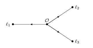 Figure 1
Peer Reviews
No public reviews on file for this paper yet. If you reviewed it on a platform where reviews are public (OpenReview, ICLR, NeurIPS, ICML), you can paste yours below so the community can read it here.
Videos
No videos yet. Explain this paper in a talk, walkthrough, or lecture? Add one.
Feedback stabilization and boundary controllability of the Korteweg-de Vries equation on a star-shaped network
Kaïs Ammari
UR Analysis and Control of PDEs, UR 13ES64, Department of Mathematics, Faculty of Sciences of Monastir, University of Monastir, Tunisia and Laboratoire de Mathématiques, Université de Versailles Saint-Quentin en Yvelines, 78035 Versailles, France and Université Paris-Saclay, France
and
Emmanuelle Crepeau
Laboratoire de Mathématiques, Université de Versailles Saint-Quentin en Yvelines, 78035 Versailles, France
Abstract.
We propose a model using the Korteweg-de Vries equation on a finite star-shaped network. We first prove the well-posedness of the system and give some regularity results. Then we prove that the energy of the solutions of the dissipative system decays exponentially to zero when the time tends to infinity. Lastly we show an exact boundary controllability result.
Résumé. On propose dans cet article un modèle de l’équation de Korteweg-de Vries sur un réseau sous forme d’une étoile. On prouve que le problème est bien posé et on établit quelques propriétés de régularité. De plus, on montre que l’énergie du système décroit d’une manière exponentielle vers [math] quand le temps tend vers l’infini. A la fin, on déduit un résultat de contrôlabilité frontière du système associé.
Key words and phrases:
Star-Shaped Network, KdV equation, stabilization, controllability
2010 Mathematics Subject Classification:
35L05, 35M10
Contents
-
3.1.1 Observability inequality and stability in the non critical case
-
3.2 Stabilization of the system on a star-shaped network in the critical or non critical case
1. Introduction
In the last few years various physical models of multi-link flexible structures consisting of finitely many interconnected flexible elements such as strings, beams, plates, shells have been mathematically studied. For details about some physical motivation for the models, see [11, 3, 4, 1] and the references therein.
In [10], the Korteweg-de Vries equation (KdV) is designed for modeling the pressure in an arterial compartment. Indeed, the Korteweg-de Vries equation models usually long waves in a channel of relatively shallow depth. Thus we propose a new model using this nonlinear dispersive partial differential equation on a network to be used to model the pressure on the arterial tree.
Numerous papers on the stability or the exact controllability of the KdV equation on a finite length interval have already been studied, see for example [15, 13] for the stability and [16, 8, 6, 7] for the control problem. In [6], a tutorial of both problems is presented.
To our knowledge, there is no work about the KdV equation on a star-network but we can cite the article [9] where the controllability of the KdV equation on a compartment with nodes is presented.
Now, let us first introduce some notations and definitions which will be used throughout the rest of the paper, in particular some which are linked to the notion of - networks, (as introduced in [11]).
Let be a connected topological graph embedded in ℝ, with edges (). Let be the set of the edges of . Each edge is a Jordan curve in ℝ and is assumed to be parametrized by its arc length such that the parametrization is -times differentiable, i.e. for all . The - network associated with is then defined as the union
[TABLE]
We define by , the maximal length of the network.
We study here the stabilization problem and the controllability one of a KdV system on a star-shaped network as in the following figure for .
More precisely, we study a system which is in connection with the mathematical modeling of the human cardiovascular system. For each edge , the scalar function for and contains the information on the displacement of the wave at location and time , .
We consider the evolution problems and described by the following systems:
[TABLE]
and
[TABLE]
where .
We define the natural energy of a solution of or system by
[TABLE]
We can easily check that every sufficiently smooth solution of satisfies the following dissipation law
[TABLE]
and therefore, the energy is a nonincreasing function of the time variable .
This paper is organized as follows: In Section 2, we give the proper functional setting for both systems and and prove that those systems are well-posed. We also give some regularity results. In Section 3, we prove our main results, namely the stabilization problem of the systems given by and . For doing this, we derive first an observability inequality for the linear system and then we apply a fixed point theorem for the non-linear one. In the last Section 4 we prove that the observability inequality also gives the controllability result in the case where the network is non critical.
2. Well-posedness and regularity results
In order to study both systems on the network, we need a proper functional setting. We define the following spaces:
[TABLE]
[TABLE]
and
[TABLE]
equipped with the inner product
[TABLE]
We also define the following space endowed with the norm
[TABLE]
2.1. Well-posedness of the system and regularity results
The system can be rewritten as the first order evolution equation
[TABLE]
where is the vector and the operator is defined by
[TABLE]
[TABLE]
and
[TABLE]
Now we can prove, according to the linear semi-group theory (see [14]), the well-posedness of system and that the solution satisfies the dissipation law (1.2).
Proposition 2.1**.**
For an initial datum , there exists a unique solution to problem (2.4). Moreover, the solution satisfies (1.2). Therefore the energy is decreasing.
Proof.
The operator is clearly closed. Let , then by using some integration by parts, we get,
[TABLE]
Thus is dissipative.
The adjoint operator of is defined by with
[TABLE]
In the same manner, we obtain,
[TABLE]
hence is also dissipative and then generates a strongly semi-group of contractions on . We denote by this semi-group.
∎
We also need some regularity results for the solution of the linear equation with some extra boundary conditions,
[TABLE]
Proposition 2.2**.**
Let , where . Then there exists a unique solution of (2.5).
Proof.
We first define the functions . Thus and satisfies,
[TABLE]
We define , then satisfies the system:
[TABLE]
Thus, as , we deduce from Proposition 2.1 and classical results on semi-group theory, that system (2.6) admits a unique classical solution . Hence we can easily prove that problem (2.5) admits a unique classical solution .
∎
Now, we study the same system but with less regular data.
Proposition 2.3**.**
Let , then there exists a unique mild solution of (2.20), . Furthermore and belong to and we have the following estimates,
[TABLE]
[TABLE]
[TABLE]
Proof.
The proof of this result is obtained by a density argument and the multiplier method. We first suppose that and thus the solution of (2.5) satisfies .
Let .Then by multiplying by , integrating on with and using some integrations by parts we get the following equation,
[TABLE]
- (1)
Taking first , then (2.10) becomes,
[TABLE]
So we have,
[TABLE]
[TABLE]
Thus, and we have the estimate,
[TABLE]
Taking in inequality (2.11) gives that and , for all and we have the estimates,
[TABLE] 2. (2)
Secondly, we take for and then equation (2.10) gives us,
[TABLE]
Then we have,
[TABLE]
Using estimates (2.12) and (2.13), we can deduce the following estimate,
[TABLE] 3. (3)
Lastly, we choose for and then we obtain the equation,
[TABLE]
and then we easily get
[TABLE]
By the density of in and of in , and by using inequalities (2.12), (2.13) and (2.14), we get the desired result. ∎
Before proving the well-posedness of we need also a result of regularity for the linear system with a source term.
Proposition 2.4**.**
Let , then there exists a unique mild solution of
[TABLE]
and it satisfies,
[TABLE]
Proof.
Thanks to Proposition 2.3, we consider that . By using standard semi-group theory, we get that if then the solution of (2.15) verifies and
[TABLE]
As before we multiply the PDE in (2.15) by and we integrate by parts on . We easily obtain that,
[TABLE]
Thus
[TABLE]
Next, we multiply the PDE in (2.15) by and integrate by parts. We obtain,
[TABLE]
Thanks to (2.17), we obtain that,
[TABLE]
Which ends the proof. ∎
2.2. Well-posedness of and regularity results
In order to prove the well-posedness of the nonlinear KdV equation, we need some regularity on the nonlinearity appearing in the equation and at the central node.
We first recall the following Proposition whose proof can be found in [16, Proposition 4.1] or [6, Proposition 4].
Proposition 2.5**.**
Let , let . Then and the map is continuous. Moreover, we have
[TABLE]
We also need the following proposition,
Proposition 2.6**.**
Let , then and the map is continuous. Moreover, we have the estimate,
[TABLE]
Proof.
Let . As we have
[TABLE]
Thus,
[TABLE]
[TABLE]
[TABLE]
[TABLE]
We get the desired result and estimate (2.19).∎
With those both previous Propositions, we can prove the well-posedness of the non-linear KdV system.
Theorem 2.7**.**
Let and . Then there exist and such that for all with , then there exists a unique solution of (KdV) that satisfies .
Proof.
Let us fix such that where will be chosen later. We prove this theorem by using the Banach fixed point Theorem on the following map, , where is the solution of,
[TABLE]
Clearly, is a solution of (KdV) is equivalent to is a fixed point of . By using the previous regularity results, namely Propositions 2.4, 2.5 and 2.6, we get that for all ,
[TABLE]
and for all ,
[TABLE]
Let us choose to be defined later and , and , then we have
[TABLE]
Thus by taking such that and such that we get the well-posedness result with the Banach fixed point Theorem. ∎
3. Exponential stability
3.1. Exponential stability of
In this section we will study two cases. First when the number of lengths which are in the space of critical lengths, namely , is strictly less than two. And in the second case when this number is larger than two.
3.1.1. Observability inequality and stability in the non critical case
Theorem 3.1**.**
Let such that . Then for all , there exists such that for all we have,
[TABLE]
where is the solution of .
Proof.
We follow the proof of Lemma 3.5 in [16] or Proposition 8 in [6]. Let us suppose that the result is false. Then we could find a sequence such that and such that
[TABLE]
where .
By using estimates (2.7) we have
[TABLE]
Thus is bounded in and then is bounded in . Thanks to the Aubin-Lions Lemma, we can deduce that is relatively compact in and we can assume that converges in .
With inequality (2.9), we have
[TABLE]
As the two last terms tends to [math] as tends to infinity, is a Cauchy sequence in and then converges to a function satisfying . Then, we have , and .
With the same type of proof as in [16], we have to prove the following Lemma:
Lemma 3.2**.**
Let . Let us consider the following assertion:
[TABLE]
Then .
Proof.
Let us first recall Lemma 3.5 in [16]:
Lemma 3.3**.**
[16, Lemma 3.5]** Let . Consider the following assertion,
[TABLE]
Then .
- (1)
If then Lemma 3.3 gives us . 2. (2)
If , then we can suppose that and for all . Then Lemma 3.3 gives us that for all , and then has to satisfy,
[TABLE]
Due to the three null conditions at the spatial origin [math], the unique solution of this system is .
Thus . 3. (3)
If , then we can suppose that . Then we can take for . Lemma 3.3 gives us two non null functions and that satisfy
[TABLE]
We then define
[TABLE]
As and are non null satisfy an ODE of order 3 and and then and . Then is non null and satisfies the system given in (3.22).
∎
From this Lemma, we easily deduce the observability inequality (3.21) and this ends the proof of Theorem 3.1. ∎
We can now prove the result of stability.
Theorem 3.4**.**
Let such that , then there exists and such that for all the solution of satisfies,
[TABLE]
Proof.
We follow the proof given in [15]. With (1.2) we have by integration and using the previous observability inequality (3.21),
[TABLE]
Thus we get easily the stability result.
∎
3.1.2. Stability in the critical case
We suppose in this section that then adding a damping mechanism on the critical branches except at most one gives the stability of the system.
Let us define , the set of critical indexes, and equals to minus one index. We study the following problem,
[TABLE]
where and the damping is defined by
[TABLE]
We can prove the well-posedness of this system as in [15], by considering it as a perturbation of (LKdV). With same types of arguments we get the stability result.
Theorem 3.5**.**
Assume that the damping is defined as in (3.24), then there exist and such that for all , the solution of satisfies,
[TABLE]
Proof.
We first multiply the PDE of by and we easily get the following estimate,
[TABLE]
Then we multiply the PDE of by to get,
[TABLE]
We argue by contradiction to prove the following inequality,
[TABLE]
By following the same arguments as for the proof of Theorem 3.1 we can construct a sequence such that the corresponding solution of satisfies
[TABLE]
By passing to the limit we obtain a non trivial solution of such that
[TABLE]
- (1)
For all , is solution of and such that . Then thanks to Lemma 3.3, . 2. (2)
For all , , thus and in . Then and thanks to Holmgren’s Theorem, . 3. (3)
For , satisfies,
[TABLE]
Due to the three null conditions at the central node, we obtain that .
Thus and we get a contradiction which ends the proof of Theorem 3.5.
∎
3.2. Stabilization of the system on a star-shaped network in the critical or non critical case
3.2.1. Stability for small amplitude solutions
In this section we study the stabilization of the non linear system for the critical and the non critical case.
We define as before , the set of critical indexes, and equals to minus one index. Eventually, . We study the following problem,
[TABLE]
where and the damping is defined by
[TABLE]
Let such that is sufficiently small in order to have with Theorem 2.7 the existence and unicity of solution of which is a perturbation of . Then we can decompose into respective solutions of
[TABLE]
[TABLE]
Then thanks to Theorems 3.4 and 3.5 we have the existence of such that for all ,
[TABLE]
Thanks to Propositions 2.4, 2.5 and 2.6 we can deduce that
[TABLE]
We need some estimates on this last right term.
We first multiply the equation of by and integrate in space and time over to obtain
[TABLE]
Secondly, we multiply by and integrate in space and time and obtain with the previous result,
[TABLE]
As for all , and embeds into , we have as in [6] or [15],
[TABLE]
We obtain with (3.27),
[TABLE]
This gives with the previous inequalities, the estimate,
[TABLE]
Thus by taking small enough such that if satisfies we have
[TABLE]
and we get the stability result.
3.2.2. Semi-global stability result
In this section we prove a semi-global result, provided that the damping is applied on all branches.
Let with,
[TABLE]
Then our main result of this section is:
Theorem 3.6**.**
Let , let satisfying (3.29), and let . Then for all with then there exist and such that the solution of satisfies,
[TABLE]
Proof.
To prove this result we follow the article of Pazoto [13]. Our result is based on this Unique Continuation Property of Saut and Sheurer [17].
Theorem 3.7**.**
([17, Theorem 4.2]) Let and let be a solution of
[TABLE]
such that , and where is a nonempty open subset of . Then , and .
By multiplying by and integrating on time and space, we have,
[TABLE]
[TABLE]
By integrating (3.30) over we have,
[TABLE]
Thus we just have to prove that there exists such that
[TABLE]
[TABLE]
∎
We assume that this inequality is false. Then we can find a sequence solution of with and such that
[TABLE]
Let us define and . Then satisfies the following problem,
[TABLE]
By multiplying the PDE in (3.32) by and integrating on we get
[TABLE]
Thus is bounded in .
By using (3.30), we see that . Thus is bounded in .
Then we can get as for the previous inequality (3.28),
[TABLE]
Thus is bounded in , and we can prove that for all , is a sequence of as
[TABLE]
Thus we can deduce that is bounded in and then we can extract from a subsequence that converges strongly in to a limit with and we have , , and , .
As is bounded in we can extract a sequence that converges in to a limit . Thus satisfies the following system,
[TABLE]
- (1)
If then thanks to Holmgren’s Theorem, we deduce that which is absurd. 2. (2)
If then we will apply the results of Saut and Sheurer [17] to get a contradiction. As satisfies the same equation as in [13] we can deduce that for all . Thus by applying Theorem 3.7 we get the contradiction and then the stability result.
4. Controllability results.
We first consider the following exact boundary controllability problem for the linearized KdV equation:
For any , and , for every , does there exist (N+1) controls and such that the solution of the following system, , satisfies and ?
[TABLE]
By applying the Hilbert Uniqueness Method, [12], it is well known that the exact boundary controllability is equivalent to the inequality of observability for the following backward adjoint problem.
[TABLE]
By following the same steps as done for Theorem 3.1, we can prove this observability inequality,
Theorem 4.1**.**
Let such that . Then for all , there exists such that for all we have,
[TABLE]
where is the solution of the backward adjoint problem.
Thus we get the following exact boundary controllability result, provided that the network is non critical.
Theorem 4.2**.**
Let and such that . Then for all , there exists and such that the solution of satisfies and .
By using a standard fixed point result we then prove the local exact controllability result for the non linear problem,
[TABLE]
Theorem 4.3**.**
Let and such that . Then there exists such that for all with and , there exists and such that the solution of satisfies and .
Remark 4.4**.**
If , there exists a finite dimensional space of which is unreachable for the linearized system . We could certainly prove the controllability of the non linear problem by using some power series expansion for the critical branches, following the same type of proof as [8], [5] or [7].
Remark 4.5**.**
In this last section, we prove the controllability by using (N+1) controls, acting at the external nodes and at the central node. It could be interesting to reduce the number of controls.
The reference list from the paper itself. Each links out to its DOI / PubMed record.
- 1[1] K. Ammari and S. Nicaise, Stabilization of elastic systems by collocated feedback, Lecture Notes in Mathematics, 2124, Springer, Cham, 2015.
- 2[2] K. Ammari, D. Mercier, V. Régnier and J. Valein, Spectral analysis and stabilization of a chain of serially connected Euler-Bernoulli beams and strings, Commun. Pure Appl. Anal., 11 (2012), 785–807.
- 3[3] K. Ammari and M. Jellouli, Remark in stabilization of tree-shaped networks of strings, Appl. Maths., 4 (2007), 327-343.
- 4[4] K. Ammari and M. Jellouli, Stabilization of star-shaped networks of strings, Diff. Integral. Equations, 17 (2004), 1395-1410.
- 5[5] E. Cerpa, Exact controllability of a nonlinear Korteweg-de Vries equation on a critical spatial domain, SIAM Journal on Control and Optimization , 46 (2007), 877-899.
- 6[6] E. Cerpa, Control of a Korteweg-de Vries equation: a tutorial, Math. Control Relat. Fields , 4 (2014), 45–99.
- 7[7] E. Cerpa and E. Crépeau, Boundary controllability for the nonlinear Korteweg-de Vries equation on any critical domain, Annales de l’Institut Henri Poincare (C) Non Linear Analysis , 26 (2009), 457-475.
- 8[8] J.M. Coron and E. Crépeau, Exact boundary controllability of a nonlinear Kd V equation with critical lengths, Journal of the European Mathematical Society , 6 (2004), 367-398.