Phylogenetic diversity and biodiversity indices on phylogenetic networks
Kristina Wicke, Mareike Fischer

TL;DR
This paper generalizes phylogenetic diversity measures from trees to networks, enabling conservation prioritization in complex evolutionary scenarios involving hybridization and horizontal gene transfer.
Contribution
It introduces new methods and software for calculating phylogenetic diversity and indices directly from phylogenetic networks, extending existing tree-based concepts.
Findings
Extended diversity indices to networks
Implemented software package NetDiversity
Applied methods to hybridizing fish species
Abstract
In biodiversity conservation it is often necessary to prioritize the species to conserve. Existing approaches to prioritization, e.g. the Fair Proportion Index and the Shapley Value, are based on phylogenetic trees and rank species according to their contribution to overall phylogenetic diversity. However, in many cases evolution is not treelike and thus, phylogenetic networks have come to the fore as a generalization of phylogenetic trees, allowing for the representation of non-treelike evolutionary events, such as horizontal gene transfer or hybridization. Here, we extend the concepts of phylogenetic diversity and phylogenetic diversity indices from phylogenetic trees to phylogenetic networks. On the one hand, we consider the treelike content of a phylogenetic network, e.g. the (multi)set of phylogenetic trees displayed by a network and the LSA tree associated with it. On the other…
Click any figure to enlarge with its caption.
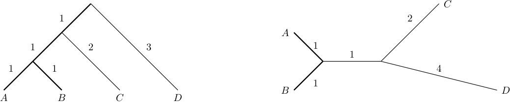 Figure 1
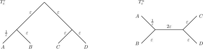 Figure 2
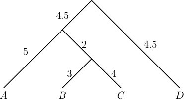 Figure 3
 Figure 4
 Figure 5
 Figure 5
 Figure 7
| X. gordoni | (1) | (3) | (3) | (4) |
|---|---|---|---|---|
| X. meyeri | (1) | (3) | (3) | (4) |
| X. continens | (3) | (1) | (1) | (2) |
| X. pygmaeus | (3) | (1) | (1) | (2) |
| X. couchianus | (5) | (7) | (5) | (8) |
| X. multilineatus | (6) | (5) | (6) | (6) |
| X. nigrensis | (6) | (5) | (6) | (6) |
| X. birchmanni | (8) | (9) | (8) | (10) |
| X. malinche | (8) | (9) | (8) | (10) |
| X. monticolus | (10) | (14) | (13) | (13) |
| X. clemenciae | (10) | (14) | (13) | (13) |
| X. alvarezi | (12) | (16) | (15) | (15) |
| X. mayae | (12) | (16) | (15) | (15) |
| X. hellerii | (14) | (18) | (18) | (18) |
| X. nezahuacoyotl | (15) | (12) | (12) | (1) |
| X. montezumae | (15) | (11) | (11) | (12) |
| X. signum | (17) | (20) | (19) | (20) |
| X. cortezi | (18) | (13) | (17) | (17) |
| X. variatus | (19) | (19) | (20) | (19) |
| X. xiphidium | (20) | (8) | (10) | (9) |
| X. evelynae | (21) | (21) | (21) | (21) |
| X. milleri | (22) | (22) | (22) | (22) |
| X. andersi | (23) | (23) | (23) | (23) |
| X. maculatus | (24) | (24) | (24) | (24) |
Peer Reviews
No public reviews on file for this paper yet. If you reviewed it on a platform where reviews are public (OpenReview, ICLR, NeurIPS, ICML), you can paste yours below so the community can read it here.
Videos
No videos yet. Explain this paper in a talk, walkthrough, or lecture? Add one.
Phylogenetic diversity and biodiversity indices on phylogenetic networks
Kristina Wicke
Mareike Fischer
Institute of Mathematics and Computer Science, University of Greifswald, Germany
Abstract
In biodiversity conservation it is often necessary to prioritize the species to conserve. Existing approaches to prioritization, e.g. the Fair Proportion Index and the Shapley Value, are based on phylogenetic trees and rank species according to their contribution to overall phylogenetic diversity. However, in many cases evolution is not treelike and thus, phylogenetic networks have been developed as a generalization of phylogenetic trees, allowing for the representation of non-treelike evolutionary events, such as hybridization. Here, we extend the concepts of phylogenetic diversity and phylogenetic diversity indices from phylogenetic trees to phylogenetic networks. On the one hand, we consider the treelike content of a phylogenetic network, e.g. the (multi)set of phylogenetic trees displayed by a network and the so-called lowest stable ancestor tree associated with it. On the other hand, we derive the phylogenetic diversity of subsets of taxa and biodiversity indices directly from the internal structure of the network. We consider both approaches that are independent of so-called inheritance probabilities as well as approaches that explicitly incorporate these probabilities. Furthermore, we introduce our software package NetDiversity, which is implemented in Perl and allows for the calculation of all generalized measures of phylogenetic diversity and generalized phylogenetic diversity indices established in this note that are independent of inheritance probabilities. We apply our methods to a phylogenetic network representing the evolutionary relationships among swordtails and platyfishes (Xiphophorus: Poeciliidae), a group of species characterized by widespread hybridization.
keywords:
Hybridization , Phylogenetic networks , Phylogenetic diversity , Shapley Value , Fair Proportion Index
1 Introduction
Facing a major extinction crisis and the inevitable loss of biodiversity at the same time with limited financial means, biological conservation has to prioritize the species to conserve. In this matter, the so-called phylogenetic diversity (Faith [1]) has been introduced as a measure of biodiversity based on the evolutionary history of species. It serves as a basis for biodiversity indices used in taxon prioritization, e.g. the Fair Proportion Index and the Shapley Value (Haake et al. [2], Hartmann [3], Fuchs and Jin [4], Wicke and Fischer [5]).
Both phylogenetic diversity, as well as the Fair Proportion Index and the Shapley Value are based on phylogenetic trees and thus, assume the evolutionary history of species to be treelike. However, there are several forms of non-treelike evolution, such as hybridization, affecting a variety of species. Therefore, phylogenetic reticulation networks have become an important concept in evolutionary biology, allowing for the representation of non-treelike evolution.
Here, we aim at combining both approaches, i.e. we aim at extending the concept of phylogenetic diversity and its measures from phylogenetic trees to phylogenetic networks. So far, phylogenetic diversity and the Shapley Value have been considered for so-called split networks, which can be used to represent conflict in data (Chernomor et al. [6], Volkmann et al. [7]), but no attempts have been made towards the generalization of phylogenetic diversity and its measures to reticulation networks.
In this note we first recapitulate phylogenetic diversity, the Fair Proportion Index and the Shapley Value on phylogenetic trees, before we focus on generalizing these concepts to phylogenetic networks.
We will introduce a variety of definitions for generalized phylogenetic diversity, following three main principles: the calculation of spanning arborescences and subgraphs of a network, the consideration of the (multi)set of phylogenetic trees displayed by a network and the construction of the so-called lowest stable ancestor tree associated with a network.
We will then turn our attention to the Fair Proportion Index and the Shapley Value and suggest different ways of using them as taxon prioritization tools in the context of phylogenetic networks.
Both for the generalized measures of phylogenetic diversity and the generalized biodiversity indices, we develop both approaches that are independent of so-called inheritance probabilities as well as approaches that explicitly incorporate these probabilities.
In case of the former, all approaches are implemented in our new software tool NetDiversity, which has been made publicly available at
www.mareikefischer.de/Software/NetDiversity.zip.
Moreover, we test NetDiversity on a recently published phylogenetic network of swordtails and platyfishes (Xiphophorus: Poeciliidae), whose evolution is characterized by widespread hybridization (Solís-Lemus and Ané [8]).
2 Preliminaries
Let be a finite set of species (taxa). A rooted phylogenetic -tree is a rooted tree with root where the leaves are bijectively labeled by . is called binary if all internal nodes have degree and the root has degree . Throughout this paper, when we refer to trees, we always mean rooted phylogenetic trees. Furthermore, we assume all edges in a tree to have edge lengths greater than zero assigned to them, and we denote the length of an edge as .
Note that all edges in a rooted phylogenetic tree are directed away from the root, thus formally the treeshape of is a so-called arborescence.
Definition 1** (Arborescence).**
Let be a directed graph and let be a specified root node (of indegree 0). Then is an arborescence (rooted at ) if there is exactly one directed path from to for all nodes .
A rooted binary phylogenetic network on is a connected rooted acyclic digraph such that:
the root has outdegree 2 (and indegree 0),
- 2.
each node with outdegree 0 has indegree 1, and the set of nodes with outdegree 0 is bijectively labeled by ,
- 3.
all other nodes either have indegree 1 and outdegree 2, or indegree 2 and outdegree 1.
Nodes with indegree 2 and outdegree 1 are called reticulation nodes and all other nodes are called tree nodes. Furthermore, tree nodes with outdegree 0 are referred to as leaves. Edges directed into a reticulation node are called reticulation edges and edges directed into a tree node are called tree edges. When we refer to phylogenetic networks, we always mean rooted binary phylogenetic networks. Moreover, when we refer to the size of a tree or a network, we mean the number of taxa, i.e. the number of leaves of the tree or network under consideration.
Additionally, we assume all tree edges of a phylogenetic network to have edge lengths greater than zero assigned to them and denote the length of a tree edge as . W.l.o.g. we define the edge lengths of all reticulation edges to be zero. However, we assign so-called inheritance probabilities to the reticulation edges of a network, reflecting the probability with which a hybrid species inherits its genetic material from both of its parents. More formally, let be a phylogenetic network on and let be a reticulation node, i.e. a hybrid species, with parents and . Let be the edge between and and analogously let be the edge between and . Then we use to denote the probability that inherits its genetic material (e.g. a nucleotide or a gene) from and we use to denote the probability that the genetic material is inherited from . We call and inheritance probabilities and associate with edge and with (cf. Figure 1). If no inheritance probabilities are given, we assume for all reticulation nodes . Moreover, we assign probability one to all tree edges, i.e. the probability assigned to an edge is given by
[TABLE]
Let be a phylogenetic network on and let be a phylogenetic -tree. We say that is embedded in , or that displays , if can be obtained from by deleting one of the reticulation edges for each reticulation node and suppressing resulting nodes of indegree 1 and outdegree 1. We use to denote the (multi)set of all rooted phylogenetic -trees displayed by .
Note that we receive the edge weights of an embedded tree as follows: for all formerly distinct edges that are melted into a new edge by suppressing nodes of indegree 1 and outdegree 1, we add their edge lengths, while all other edges keep their original weights. Moreover, note that if there are reticulation nodes in a rooted binary phylogenetic network on a taxon set , then there are at most phylogenetic -trees displayed by . However, this bound does not have to be sharp (cf. Figure 1).
In the following we will also need the probability of an embedded tree, which is calculated as follows:
For all calculate the unscaled probability
[TABLE]
where is the inheritance probability associated with . 2. 2.
Set (scaling factor). 3. 3.
Calculate the probability
[TABLE]
Here, the scaling factor ensures that the probabilities of all embedded trees sum up to one.
Example 1**.**
Consider the phylogenetic network on and its embedded trees and . We have and analogously and . Thus, and we retrieve the following probabilities of the embedded trees: and analogously and .
For a phylogenetic network and a node of that is not the root, we call any node that lies on all directed paths from the root to a stable ancestor of . The so-called lowest stable ancestor of is defined as the last node that is contained on all paths from the root to , excluding . Based on this terminology we can define the lowest stable ancestor tree or LSA tree (cf. Huson et al. [9], p. 140) associated with a network. Let be rooted phylogenetic network on . The LSA tree associated with is a rooted phylogenetic -tree that can be computed as follows: For each reticulation node in , remove all edges directed into and add a new edge from the lowest stable ancestor of into . Then repeatedly remove all unlabeled leaves and nodes with in- and outdegree 1, until no further such removal is possible. Note that the LSA tree associated with a binary rooted phylogenetic network is not necessarily a binary phylogenetic tree (cf. Figure 2). Note that every node in a phylogenetic network has a unique lowest stable ancestor . Thus, the LSA tree associated with a given network is the same regardless of the order that the reticulation nodes are processed in. Moreover, note that the concept of a lowest stable ancestor is not new, but has long been used in the theory of flow graphs, where the lowest stable ancestor of a node is called the immediate dominator of and the LSA tree is called the dominator tree of the flow graph (cf. Lengauer and Tarjan [10]).
In order to use the LSA tree for subsequent phylogenetic diversity calculations, we have to infer edge lengths for the edges of the LSA tree. For all tree edges of that are also present in , we use their original edge weights. If during the removal of nodes of in-and outdegree 1 two formerly distinct tree edges of are melted into a new edge in , we add their original edge lengths. For all newly established edges between a reticulation node and its lowest stable ancestor, we suggest to set the length of these edges to the average path length of a path between and , respectively, i.e. we set
[TABLE]
where is the set of all --paths in and the length of any such path is obtained by adding the edge lengths of all edges that are part of this path (cf. Figure 2).
Remark**.**
Note that instead of using the average path length between a reticulation node and its lowest stable ancestor in order to infer a weight for the edge , we could also use the length of a shortest path, the length of a most likely path or a weighted average path length, where each path is weighted according to its probability
[TABLE]
2.1 Phylogenetic diversity and phylogenetic diversity indices on trees
In this section we briefly recapitulate the concept of phylogenetic diversity and phylogenetic diversity indices, in particular the Shapley Value and the Fair Proportion Index, for phylogenetic trees.
Definition 2** (Phylogenetic diversity).**
Let be a rooted phylogenetic tree with leaf set . For a subset of taxa, the phylogenetic diversity is calculated by summing up the edge lengths of the phylogenetic subtree of containing and the root (i.e., we consider the sum of edge lengths in the smallest spanning tree containing and the root).
Example 2**.**
Consider the phylogenetic tree on depicted in Figure 1. Now consider the subset of taxa. Then the phylogenetic diversity of calculates as .
Based on phylogenetic diversity, we can now define the Shapley Value for phylogenetic trees. The Shapley Value for phylogenetic trees is used in different versions in the literature (cf. Wicke and Fischer [5]), but we will use the so-called original Shapley Value throughout this paper.
Definition 3** (Original Shapley Value).**
Let be a rooted phylogenetic tree with leaf set and let denote the phylogenetic diversity of . Then the Shapley Value for a taxon is defined as
[TABLE]
where and denotes a subset of species containing taxon (also sometimes referred to as ‘coalition’) and the sum runs over all such coalitions possible.
While the Shapley Value reflects the average contribution of a species to overall phylogenetic diversity and is thus a sensible prioritization criterion, its calculation is complicated. Therefore another index, the so-called Fair Proportion Index, has been introduced.
Definition 4** (Fair Proportion Index).**
For a rooted phylogenetic tree with leaf set the Fair Proportion Index of a taxon is defined as
[TABLE]
where the sum runs over all edges on the path from to the root and denotes the number of leaves descendent from that edge.
The Fair Proportion Index can easily be calculated, but lacks a biological motivation. However, its use has been justified by its equivalence with the original Shapley Value.
Theorem 1** (Fuchs and Jin [4]).**
Let be a rooted phylogenetic tree with leaf set . Then we have for all
[TABLE]
Example 3**.**
Consider the phylogenetic tree on depicted in Figure 1. Here, we have and . Note that , which equals the total sum of all edge lengths in . Also note that the Fair Proportion Indices of equal the Shapley Values of .
3 Generalization of phylogenetic diversity
We are now in the position to present our approaches towards the generalization of phylogenetic diversity from trees to networks. We will introduce three approaches, one based on the calculation of spanning arborescences and subgraphs of a network, one based on the set of trees displayed by a network and one based on the LSA tree associated with a network.
3.1 Phylogenetic (sub)net diversity
Recall that the phylogenetic diversity of a subset of taxa of a phylogenetic -tree was calculated as the sum of branch lengths of the subtree of containing and the root. For a phylogenetic network on and a subset of taxa, there may be more than one subtree, or to be precise, more than one arborescence (because a phylogenetic network is a directed graph) containing and the root. Thus, we suggest to consider an arborescence of minimum cost, i.e. an arborescence whose weight (the sum of its branch lengths) is no larger than the weight of any other arborescence spanning and the root, and introduce the so-called phylogenetic net diversity.
Definition 5** (Phylogenetic net diversity).**
Let be a rooted phylogenetic network on some taxon set . For a subset of taxa we define the phylogenetic net diversity of as the sum of branch lengths in a minimum cost arborescence containing and the root.
Note that determining the minimum cost arborescence containing a subset of taxa and the root is formally an instance of the so-called directed Steiner tree problem or Steiner arborescence problem, which, in general, is an -hard problem (Karp [11]).
In order to explicitly incorporate the inheritance probabilities of a network into the calculation of phylogenetic net diversity, several alterations of Definition 5 are possible. Instead of considering a minimum cost arborescence spanning the taxa in and the root, we could consider all arborescences spanning and the root and weight them according to their probability or use a most likely arborescence. We denote these values by and , i.e.
[TABLE]
where denotes the set of all arborescences spanning and the root, is the sum of branch lengths of any such arborescence and
[TABLE]
denotes its probability. Moreover,
[TABLE]
If the argmax is not unique, we choose one of the most likely arborescences of minimum cost.111Alternatively, we could arbitrarily choose one of the most likely arborescences. However, choosing an arborescence of minimum cost makes the results reproducible.
Example 4**.**
Consider Figure 3, which depicts the rooted phylogenetic network on and the two arborescences and containing and the root. has weight , while has weight . Thus, is the minimum cost arborescence containing and the root and we retrieve the phylogenetic net diversity of as . However, has probability and has probability , i.e. is the most likely arborescence spanning and the root. Thus, . Moreover, .
Instead of using spanning arborescences to define the phylogenetic diversity of a subset of taxa of a phylogenetic network on , we can also consider the subgraph containing the root of and and define the phylogenetic diversity of as the sum of branch lengths in .
Definition 6** (Phylogenetic subnet diversity).**
Let be a rooted phylogenetic network on some taxon set . For a subset of taxa consider the subgraph of containing the root of and the taxa in (i.e., is the subgraph of containing all nodes and edges that lie on at least one path from the root of to any of the leaves in ). Then we define the phylogenetic subnet diversity of as the sum of branch lengths in .
Example 5**.**
Consider the rooted phylogenetic network on depicted in Figure 3 and set . Then the subgraph of (highlighted with bold lines) has length and thus, .
3.2 Embedded phylogenetic diversity
If species are subject to hybridization or horizontal gene transfer, their genome contains parts of the genome of both its ancestors. However, evolution at the nucleotide level rather than the genome level is still treelike, because a single nucleotide can always be traced back to one parent. Therefore, we suggest to consider the set of trees embedded in a network as an alternative approach towards the generalization of phylogenetic diversity from trees to networks.
Definition 7** (Embedded phylogenetic diversity).**
Let be a rooted phylogenetic network on some taxon set and let be the (multi)set of all rooted phylogenetic -trees displayed by . Then we use to denote the embedded phylogenetic diversity of a subset of taxa, where is one of the following functions and define
[TABLE]
where is the number of phylogenetic -trees displayed by . If inheritance probabilities are given for , we also consider
[TABLE]
where is the probability of and is a most likely embedded tree. If the argmax is not unique, we arbitrarily choose one of the embedded trees with maximum probability.
Note that can be replaced by other functions on the phylogenetic diversity of the trees in , but we will only consider and as defined above.
Also note that we will only consider phylogenetic -trees as elements of and discard all other trees that may occur when decomposing the network into a set of trees (cf. Figure 1).
Example 6**.**
Consider the rooted phylogenetic network on and its embedded trees and depicted in Figure 1. Now set . Then we have and . Moreover, and . Thus, we retrieve the different values of the embedded phylogenetic diversity of as and .
3.3 Relationship between the phylogenetic net diversity and the embedded phylogenetic diversity
Comparing the phylogenetic net diversity and the minimum embedded phylogenetic diversity for a subset of taxa, we see that they use a similar principle. While is defined as the weight of a minimum cost arborescence spanning and the root in a network , is defined as the weight of a minimum spanning tree/minimum cost arborescence spanning and the root in the set of phylogenetic -trees displayed by . Thus, the two measures are related, but in general they are not identical. Consider, for example the rooted phylogenetic network depicted in Figure 1 and set . Then, we have , while .
However, we have the following relationship between and :
Proposition 1**.**
Let be a binary rooted phylogenetic network on a taxon set with reticulation nodes and let be the set of phylogenetic -trees displayed by .
We have
[TABLE]
for all subsets of taxa. 2. 2.
If , i.e. if all combinations of removing one reticulation edge for each reticulation node and suppressing nodes of both indegree 1 and outdegree 1 result in a phylogenetic -tree, we have
[TABLE]
Remark**.**
Note that for example holds for so-called normal networks (cf. van Iersel et al. [12]).
Proof of Proposition 1.
Let be a binary rooted phylogenetic network with root , taxon set and reticulation nodes. Let be the set of embedded trees and let be the set of reticulation nodes of .
We show .
For every the phylogenetic diversity of a subset of taxa is defined as the sum of branch lengths in the smallest arborescence spanning the taxa in and the root. Clearly, the weight of any such arborescence cannot be smaller than the weight of a minimum cost arborescence spanning and the root in (all are “subgraphs” of , thus, any smallest arborescence spanning and the root in a displayed tree can also be found in ).222Formally, we have to re-establish the nodes of in- and outdegree 1 that were removed during the construction of to make a subgraph of . However, this does not affect the weights. In particular, we have
[TABLE] 2. 2.
Now, suppose that . We want to show that . As we have (Equation (9)), it suffices to show .
Let be the minimum cost arborescence spanning and the root in . By definition of an arborescence there is exactly one directed path from the root to any other vertex . This implies that contains at most one reticulation edge for each reticulation node , but never both reticulation edges directed into . If we now suppress nodes of both indegree 1 and outdegree 1 in and add the weights of the edges which are merged into one edge by doing so, we retrieve a directed acyclic graph , which contains the taxa in and whose weight equals the weight of . By the construction of , however, must be a sub-arborescence of some embedded tree , where the set of embedded trees is obtained by deleting one of the reticulation edges for each reticulation node and suppressing the resulting nodes of indegree 1 and outdegree 1, and every combination of doing so results in a phylogenetic -tree (because we have assumed ). Thus, by definition of for trees, the weight of equals and as is embedded in we have
[TABLE]
Combining the above, we have as claimed.
∎
Comparing and of a subset of taxa, we see that these values, again, follow a related principle. While considers all spanning arborescences in the network, considers the spanning arborescences in each of the trees displayed by . If , the two values coincide (proof similar to the proof of Proposition 1). However, in general, , in particular we cannot guarantee as in Proposition 1. Consider for example the phylogenetic network depicted in Figure 1 and set . Then we have
[TABLE]
but
[TABLE]
Thus, .
3.4 LSA associated phylogenetic diversity
As it can be difficult to determine the set of phylogenetic -trees displayed by a network on , we now consider the LSA tree associated with a network. The LSA tree can be seen as a way to summarize the treelike content of a phylogenetic network, on which all its embedded trees agree, without explicitly having to consider these trees.
Definition 8** (LSA associated phylogenetic diversity).**
Let be a rooted phylogenetic network on some taxon set . Let be a subset of taxa. Then we define the LSA associated phylogenetic diversity as
[TABLE]
where is the phylogenetic diversity of in the LSA tree associated with .
Example 7**.**
Consider the rooted phylogenetic network and its associated LSA tree depicted in Figure 2. Exemplarily, we set and retrieve the LSA associated phylogenetic diversity of as .
We have introduced a variety of ways to define the phylogenetic diversity of a subset of taxa in a network. However, the information about the phylogenetic diversity of a subset of taxa in itself is not very useful for taxon prioritization decisions. Thus, we now turn our attention towards the generalization of phylogenetic diversity indices from trees to networks.
4 Generalization of phylogenetic diversity indices
After proposing different ways of generalizing the concept of phylogenetic diversity from trees to networks, we will now turn our attention to the Fair Proportion Index and the Shapley Value, two prioritization indices used in biodiversity conservation. Even though the Fair Proportion Index and the Shapley Value are equivalent for rooted phylogenetic trees (Fuchs and Jin [4]), they differ significantly in their definition and computation. While the Fair Proportion Index is directly based on a given rooted phylogenetic tree (cf. Definition 4), the definition of the Shapley Value is based on the phylogenetic diversity of subsets of taxa, and thus, only indirectly on a given phylogenetic tree (cf. Definition 3). To be precise, the calculation of the Shapley Value involves two steps:
Calculation of the phylogenetic diversity for all subsets of taxa based on a given phylogenetic tree. 2. 2.
Calculation of the Shapley Value for all taxa based on the phylogenetic diversity calculated in step 1.
This implies that we have two possibilities when extending the Shapley Value from trees to networks: We can either use any generalized definition of phylogenetic diversity (e.g. the phylogenetic net diversity, the embedded phylogenetic diversity or the LSA associated phylogenetic diversity) introduced above and calculate the Shapley Value based on this measure, or we can reduce the network to its treelike content (e.g. via the set of embedded trees or the LSA tree) and calculate the Shapley Value based on these trees. We will, however, start with the reduction of a network to its treelike content, which is also used to generalize the Fair Proportion Index to networks.
4.1 Embedded Shapley Value and Fair Proportion Index
Similar to the embedded phylogenetic diversity, we will now use the set of phylogenetic -trees displayed by a network on in order to define the so-called embedded Shapley Value and the embedded Fair Proportion Index.
Definition 9** (Embedded Shapley Value, embedded Fair Proportion Index).**
Let be a rooted phylogenetic network on some taxon set and let be the (multi)set of all rooted phylogenetic -trees displayed by . Then we use with to denote the embedded Shapley Value or embedded Fair Proportion Index of a taxon , where stands for and define
[TABLE]
where is the number of phylogenetic -trees displayed by . If inheritance probabilities are given for , we also consider
[TABLE]
where is the probability of and is a most likely embedded tree. If the argmax is not unique, we arbitrarily choose one of the embedded trees with maximum probability.
Note that as the Shapley Value and the Fair Proportion Index are equivalent on rooted phylogenetic trees (Fuchs and Jin [4]), the embedded values coincide as well, i.e. etc.
Example 8**.**
Consider the rooted phylogenetic network on and its embedded trees and depicted in Figure 1 and fix taxon . Then we have and . Moreover, and . Thus, we retrieve the different versions of the embedded Fair Proportion Index of as and .
4.2 LSA associated Shapley Value and Fair Proportion Index
An alternative way of reducing a phylogenetic network to its treelike content is the LSA tree. Thus, we will now introduce the LSA associated Shapley Value and the LSA associated Fair Proportion Index.
Definition 10** (LSA associated Shapley Value, LSA associated Fair Proportion Index).**
Let be a rooted phylogenetic network on some taxon set . Let be a taxon in . Then we use with to denote the LSA associated Shapley Value or LSA associated Fair Proportion Index and define
[TABLE]
where is the respective diversity index (i.e. the Shapley Value or the Fair Proportion Index) in the LSA tree associated with .
Obviously, , because the two values coincide for rooted phylogenetic trees, thus they coincide in particular for the LSA tree.
Example 9**.**
Consider the rooted phylogenetic network and its associated LSA tree depicted in Figure 2 and fix taxon . Then the LSA associated Fair Proportion Index of is .
4.3 Generalized Shapley Value
As the definition of the Shapley Value is only indirectly based on a given phylogenetic -tree and just requires a measure of phylogenetic diversity for all subsets of taxa (cf. Definition 3), we now introduce an alternative way of calculating the Shapley Value for the taxa of a phylogenetic network . We suggest to calculate the Shapley Value according to its definition and use any measure of generalized phylogenetic diversity (e.g. the phylogenetic net diversity, the embedded phylogenetic diversity or the LSA associated phylogenetic diversity) as an input. We call the resulting value the generalized original Shapley Value.
Definition 11** (Generalized Shapley Value).**
Let be a rooted phylogenetic network on some taxon set and let be the (multi)set of all rooted phylogenetic -trees displayed by . Let be a taxon in and let denote any generalized measure of phylogenetic diversity of a subset of taxa in , i.e. .
Then we define the generalized original Shapley Value of as
[TABLE]
where and denotes a subset of species containing taxon and the sum runs over all such subsets possible.
Example 10**.**
Consider the rooted phylogenetic network on depicted in Figure 1. We now calculate the generalized original Shapley Value of taxon and choose the phylogenetic net diversity (cf. Definition 5) as input. We have to consider the following subsets : and . Thus,
[TABLE]
4.4 Relationship between the different versions of the Shapley Value for phylogenetic networks
We now shortly compare the generalized Shapley Value and the embedded Shapley Value of a phylogenetic network on .
The first observation to make is that, in general,
and
- 2.
for . Consider for example the rooted phylogenetic network on depicted in Figure 1 and fix taxon . Then we have and .
The second observation to make is
[TABLE]
if the most likely tree is fixed, because:
[TABLE]
Moreover, it is easy to see that for all
- (i)
, 2. (ii)
and 3. (iii)
.
Proof.
We only show (i), but (ii) and (iii) follow analogously.
Recall that . Thus,
[TABLE]
On the other hand we have
[TABLE]
Thus,
[TABLE]
∎
If we compare the LSA associated Shapley Value and the generalized Shapley Value that uses the LSA associated phylogenetic diversity as input, we see that all calculations are based upon the LSA tree associated with a network on , thus for all
- (iii)
.
4.5 Net Fair Proportion Index
Before turning to our software tool and real data, we introduce one last index concept for networks, namely the Net Fair Proportion Index. While in the previous sections we have always reduced a network on to its treelike content in order to calculate the Fair Proportion Index for its taxa (i.e. we have defined the embedded Fair Proportion Index and the LSA associated Fair Proportion Index), we now try to directly adapt the definition of the Fair Proportion Index (cf. Definition 4) to networks by considering all paths between the root and a taxon.
Without loss of generality we assume the network to come with inheritance probabilities (if no inheritance probabilities are given for , we set for all reticulation edges ).
The idea is now to define the Net Fair Proportion Index of a taxon by considering all paths from the root to and calculating a value for each path individually. Similar to the original Fair Proportion Index, we calculate this value as a weighted sum of branch lengths, where each branch length is weighted according to the number of its descendants. However, we additionally weight the possible descendants of an edge by their probability of actually being a descendant of this edge. We then use the weighted mean of these values for all paths, where a path is weighted according to its probability, and call the resulting value the Net Fair Proportion Index.
Definition 12** (Net Fair Proportion Index).**
Let be a rooted phylogenetic network on some taxon set . Let denote the length of an edge in and let denote the set of leaves that are descendants of .
For each leaf we use to denote the probability of being descendent from and calculate as
[TABLE]
where is the set of paths from the endpoint of to the leaf in and is the probability of any such path (the probability of a path is calculated as the product of all probabilities assigned to its edges).
Now let be a taxon of and let be the set of all paths from to in . Then we define the Net Fair Proportion Index of as
[TABLE]
Example 11**.**
Consider the rooted phylogenetic network on depicted in Figure 1. We now calculate the Net Fair Proportion Index for taxon :
There are two paths from the root to in , namely
[TABLE]
Consider, for example, the edge . The set of possible descendants from consists of the taxa and , thus, . The probabilities of these taxa descending from calculate as
[TABLE]
Analogously, these probabilities can be calculated for all other edges on and . Omitting edges of length 0 (i.e. hybridization edges) in the sum, we have
[TABLE]
Similar calculations yield
[TABLE]
Note that
[TABLE]
thus, the sum of the Net Fair Proportion Indices equals the sum of edge lengths in .
Remarks**.**
By definition of the Net Fair Proportion Index, this measure is efficient, i.e.
[TABLE]
where is the sum of branch lengths of the rooted phylogenetic network on .
- 2.
For a phylogenetic -tree , the Net Fair Proportion Index reduces to the original Fair Proportion Index, i.e. for all
[TABLE]
5 Software and Data
In order to calculate the different generalized measures of phylogenetic diversity and generalized diversity indices introduced above, we developed a software tool called NetDiversity, which is available from
www.mareikefischer.de/Software/NetDiversity.zip. The tool is written in the programming language Perl and uses modules from BioPerl (Stajich [13]), in particular the Bio::PhyloNetwork package (Cardona et al. [14]) The program takes networks represented in the so-called extended Newick format (Cardona et al. [15]) as an input. Depending on the options chosen, the program either outputs any measure of generalized phylogenetic diversity for all subsets of taxa or any generalized diversity index for all taxa of the network. However, currently the tool can only calculate measures independent of inheritance probabilities.
We now apply NetDiversity to a phylogenetic network of swordtails and platyfishes (Xiphophorus: Poeciliidae) (cf. Solís-Lemus and Ané [8]). This is one of the few published hybridization networks, even though hybridization is suspected to have occurred in a variety of other organisms as well. The Xiphophorus hybridization network inferred in Solís-Lemus and Ané [8] contains species and reticulation nodes (cf. Figure 4). Exemplarily, we use NetDiversity to calculate the different versions of the Fair Proportion Index for the Xiphophorus species. Note that there are possible subsets of taxa for a network on species, which is why we refrain from calculating any measure of generalized phylogenetic diversity for all subsets of Xiphophorus or the generalized Shapley value here. Table 1 summarizes the results. For the Xiphophorus network, the rankings obtained by the embedded Fair Proportion Indices and the LSA associated Fair Proportion Index are very similar. There are, however, two striking differences concerning the species X. xiphidium and X. nezahuacoyotl. While X. xiphidium is ranked low by , it is placed among the top 10 species by all other indices. The other difference between the indices concerns X. nezahuacoyotl, a hybrid species. X. nezahuacoyotl is ranked first by , while it is ranked , and by the other indices.
Thus, in case of the Xiphophorus network, the different versions of the generalized Fair Proportion Index yield similar results, but there are striking differences. In particular the question of whether hybrid species are of high or low importance for overall biodiversity remains to be considered from a biological perspective.
6 Discussion and Outlook
In this paper, we have introduced different approaches towards the generalization of phylogenetic diversity and phylogenetic diversity indices from trees to networks. Our approaches provide an extension to existing prioritization tools in conservation biology and allow for the consideration of phylogenetic networks in prioritization decisions. This is of importance if the evolutionary history of a set of species is known to be non-treelike, and thus cannot be represented by a phylogenetic tree. Here, we have mainly focused on hybridization networks, but mathematically our approaches are also applicable to networks representing horizontal gene transfer. We have applied our methods to a phylogenetic network representing the evolutionary relationships among swordtails and platyfishes (Xiphophorus: Poeciliidae), whose evolution is characterized by widespread hybridization. We have seen that different biodiversity indices may induce striking differences in the ranking order of taxa for conservation. Therefore, we remark that further research concerning the biological plausibility of our approaches is necessary before they can be put into practice. This may be achieved when more phylogenetic networks for different groups of organisms become available and can be analyzed under both a biological and mathematical perspective. Decisions in biodiversity conservation and taxon prioritization do always require thorough examination and should include as much information as possible.
Supporting Information
S1 Text. Supporting information file that contains the Xiphophorus hybridization network (Solís-Lemus and Ané [8], its LSA tree and its embedded trees.
Acknowledgements
We thank Volkmar Liebscher for helpful discussions on this research project and two anonymous reviewers for helpful comments on an earlier version of this manuscript. The first author also thanks the Ernst-Moritz-Arndt-University Greifswald for the Landesgraduiertenförderung studentship, under which this work was conducted.
References
- Faith [1992]
D. P. Faith,
Conservation evaluation and phylogenetic diversity,
Biological Conservation 61 (1992) 1–10.
- Haake et al. [2007]
C.-J. Haake, A. Kashiwada, F. E. Su,
The Shapley value of phylogenetic trees,
J. Math. Biol. 56 (2007) 479–497.
- Hartmann [2013]
K. Hartmann,
The equivalence of two phylogenetic biodiversity measures: the Shapley value and Fair Proportion index.,
J Math Biol 67 (2013) 1163–1170.
- Fuchs and Jin [2015]
M. Fuchs, E. Y. Jin,
Equality of Shapley value and fair proportion index in phylogenetic trees.,
J Math Biol 71 (2015) 1133–1147.
- Wicke and Fischer [2017]
K. Wicke, M. Fischer,
Comparing the rankings obtained from two biodiversity indices: the Fair Proportion Index and the Shapley Value,
Journal of Theoretical Biology 430 (2017) 207–214.
- Chernomor et al. [2016]
O. Chernomor, S. Klaere, A. von Haeseler, B. Q. Minh, Split Diversity: Measuring and Optimizing Biodiversity Using Phylogenetic Split Networks, Springer International Publishing, Cham, 2016, pp. 173–195. URL: http://dx.doi.org/10.1007/978-3-319-22461-9_9. doi:10.1007/978-3-319-22461-9_9.
- Volkmann et al. [2014]
L. Volkmann, I. Martyn, V. Moulton, A. Spillner, A. O. Mooers,
Prioritizing Populations for Conservation Using Phylogenetic Networks,
PLoS ONE 9 (2014) e88945.
- Solís-Lemus and Ané [2016]
C. Solís-Lemus, C. Ané,
Inferring phylogenetic networks with maximum pseudolikelihood under incomplete lineage sorting,
PLOS Genetics 12 (2016) e1005896.
- Huson et al. [2011]
D. H. Huson, R. Rupp, C. Scornavacca, Phylogenetic Networks: Concepts, Algorithms and Applications, Cambridge University Press, New York, NY, USA, 2011.
- Lengauer and Tarjan [1979]
T. Lengauer, R. E. Tarjan,
A fast algorithm for finding dominators in a flowgraph,
TOPLAS 1 (1979) 121–141.
- Karp [1972]
R. M. Karp, Reducibility among Combinatorial Problems, Springer US, Boston, MA, 1972, pp. 85–103. URL: http://dx.doi.org/10.1007/978-1-4684-2001-2_9. doi:10.1007/978-1-4684-2001-2_9.
- van Iersel et al. [2010]
L. van Iersel, C. Semple, M. Steel,
Locating a tree in a phylogenetic network,
Information Processing Letters 110 (2010) 1037 – 1043.
- Stajich [2002]
J. E. Stajich,
The Bioperl Toolkit: Perl Modules for the Life Sciences,
Genome Research 12 (2002) 1611–1618.
- Cardona et al. [2008a]
G. Cardona, F. Rosselló, G. Valiente,
A perl package and an alignment tool for phylogenetic networks,
BMC Bioinformatics 9 (2008a) 175.
- Cardona et al. [2008b]
G. Cardona, F. Rosselló, G. Valiente,
Extended Newick: it is time for a standard representation of phylogenetic networks,
BMC Bioinformatics 9 (2008b) 532.
- Huson and Scornavacca [2012]
D. H. Huson, C. Scornavacca,
Dendroscope 3: An Interactive Tool for Rooted Phylogenetic Trees and Networks,
Systematic Biology 61 (2012) 1061–1067.
The reference list from the paper itself. Each links out to its DOI / PubMed record.
- 1Faith [1992] D. P. Faith, Conservation evaluation and phylogenetic diversity, Biological Conservation 61 (1992) 1–10.
- 2Haake et al. [2007] C.-J. Haake, A. Kashiwada, F. E. Su, The Shapley value of phylogenetic trees, J. Math. Biol. 56 (2007) 479–497.
- 3Hartmann [2013] K. Hartmann, The equivalence of two phylogenetic biodiversity measures: the Shapley value and Fair Proportion index., J Math Biol 67 (2013) 1163–1170.
- 4Fuchs and Jin [2015] M. Fuchs, E. Y. Jin, Equality of Shapley value and fair proportion index in phylogenetic trees., J Math Biol 71 (2015) 1133–1147.
- 5Wicke and Fischer [2017] K. Wicke, M. Fischer, Comparing the rankings obtained from two biodiversity indices: the Fair Proportion Index and the Shapley Value, Journal of Theoretical Biology 430 (2017) 207–214.
- 6Chernomor et al. [2016] O. Chernomor, S. Klaere, A. von Haeseler, B. Q. Minh, Split Diversity: Measuring and Optimizing Biodiversity Using Phylogenetic Split Networks, Springer International Publishing, Cham, 2016, pp. 173–195. URL: http://dx.doi.org/10.1007/978-3-319-22461-9_9 . doi: 10.1007/978-3-319-22461-9\_9 . · doi ↗
- 7Volkmann et al. [2014] L. Volkmann, I. Martyn, V. Moulton, A. Spillner, A. O. Mooers, Prioritizing Populations for Conservation Using Phylogenetic Networks, P Lo S ONE 9 (2014) e 88945.
- 8Solís-Lemus and Ané [2016] C. Solís-Lemus, C. Ané, Inferring phylogenetic networks with maximum pseudolikelihood under incomplete lineage sorting, PLOS Genetics 12 (2016) e 1005896.