Probabilistic Motion Planning under Temporal Tasks and Soft Constraints
Meng Guo, Michael M. Zavlanos

TL;DR
This paper presents a probabilistic motion planning framework for mobile robots under uncertainty, optimizing task satisfaction probability and cost, with novel multi-objective control synthesis and validation through simulations and experiments.
Contribution
It introduces a multi-objective optimization approach using coupled Linear Programs for probabilistic task satisfaction and cost minimization, including a new algorithm for zero-probability scenarios.
Findings
Outperforms Round-Robin policies in trajectory suffix
Provides guarantees on probabilistic satisfaction and cost optimality
Includes a new control synthesis method for zero-probability cases
Abstract
This paper studies motion planning of a mobile robot under uncertainty. The control objective is to synthesize a {finite-memory} control policy, such that a high-level task specified as a Linear Temporal Logic (LTL) formula is satisfied with a desired high probability. Uncertainty is considered in the workspace properties, robot actions, and task outcomes, giving rise to a Markov Decision Process (MDP) that models the proposed system. Different from most existing methods, we consider cost optimization both in the prefix and suffix of the system trajectory. We also analyze the potential trade-off between reducing the mean total cost and maximizing the probability that the task is satisfied. The proposed solution is based on formulating two coupled Linear Programs, for the prefix and suffix, respectively, and combining them into a multi-objective optimization problem, which provides…
Click any figure to enlarge with its caption.
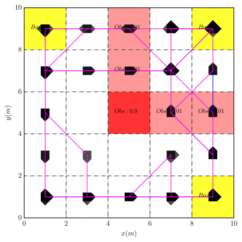 Figure 1
 Figure 2
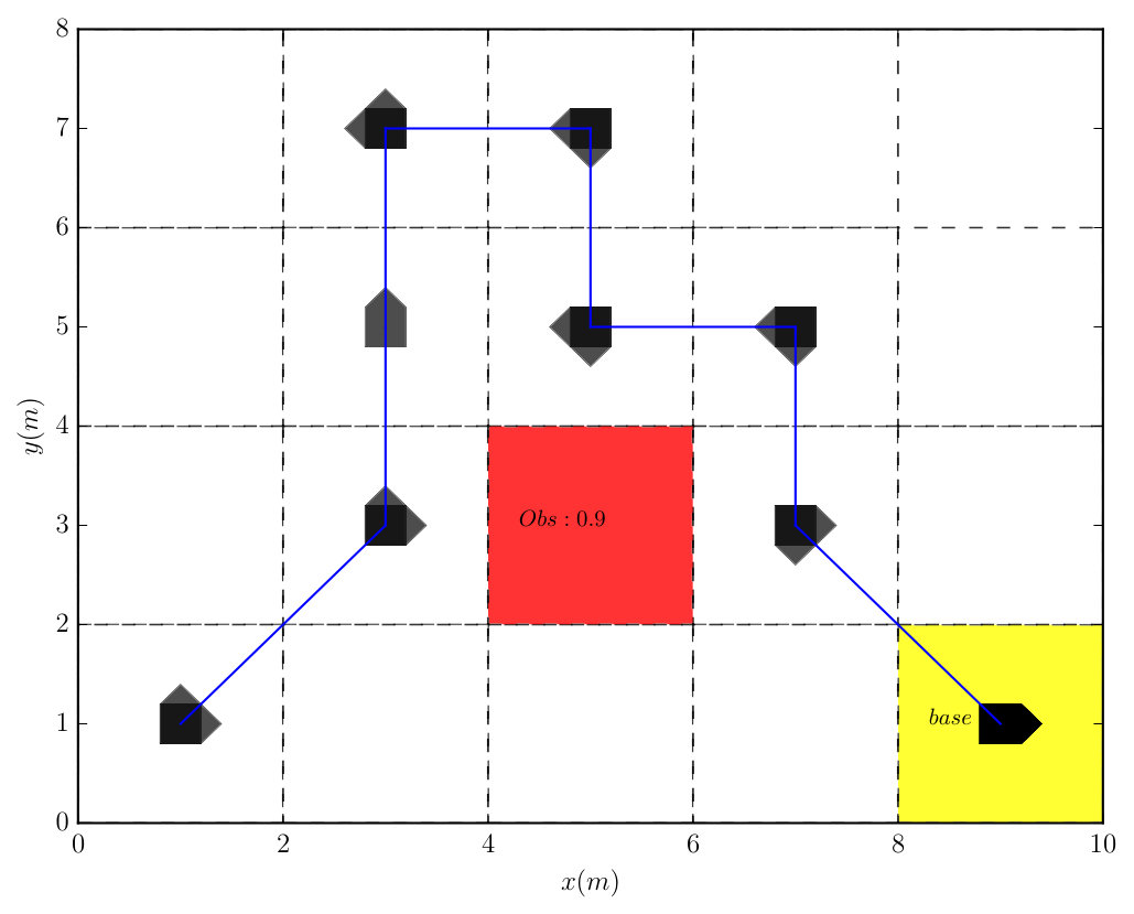 Figure 3
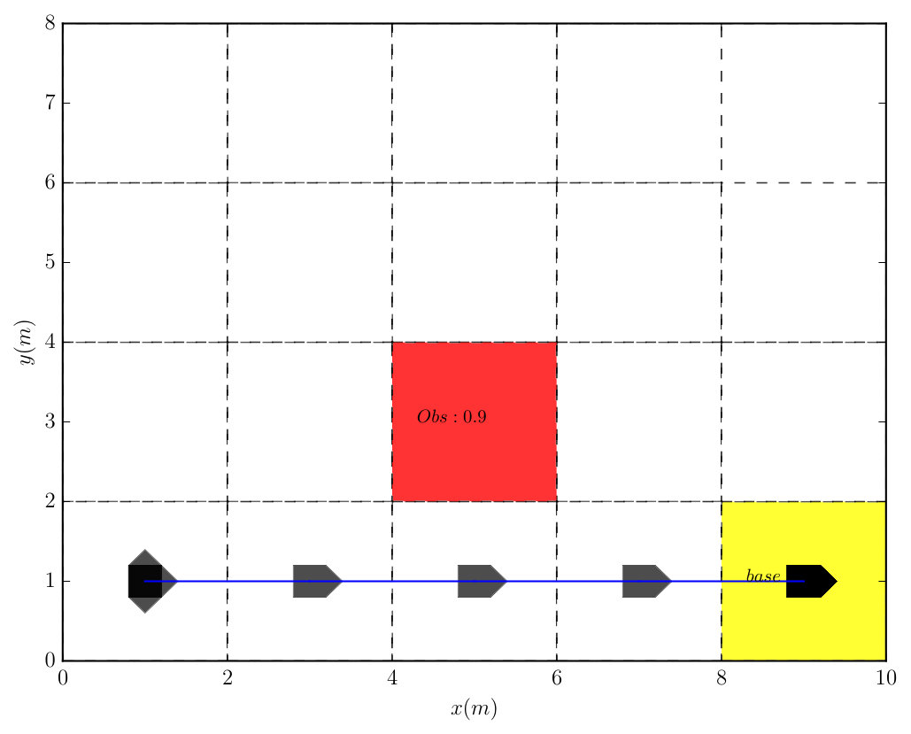 Figure 4
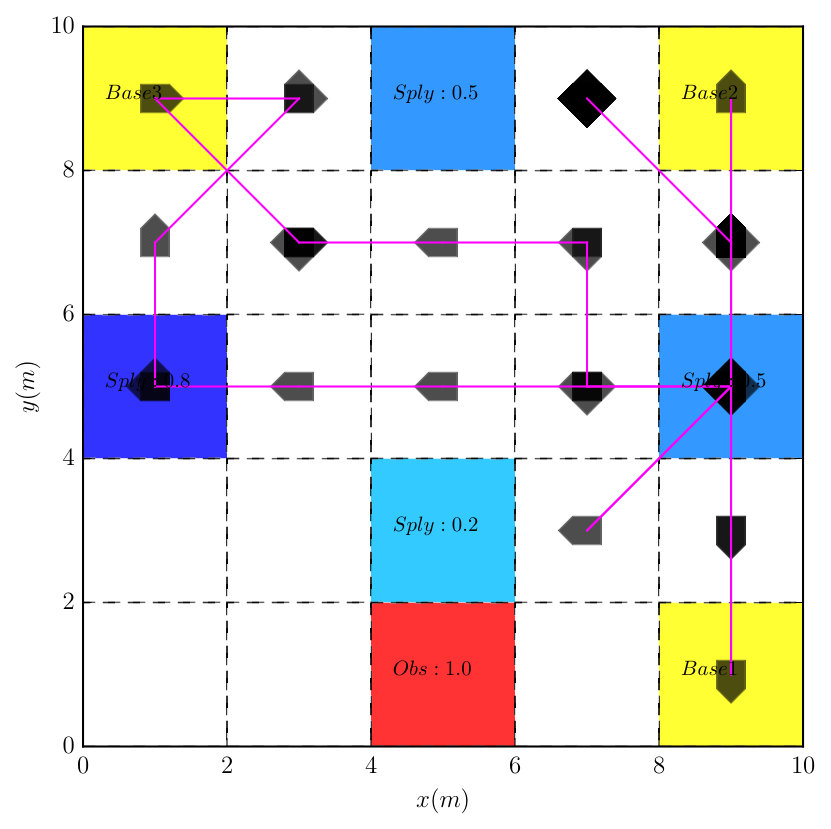 Figure 5
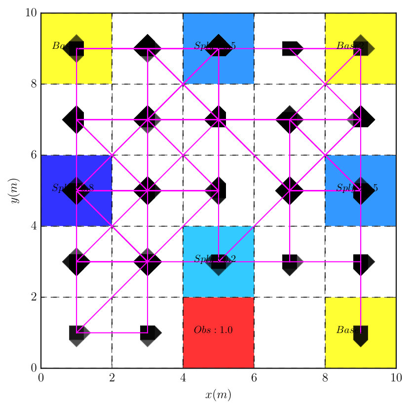 Figure 6
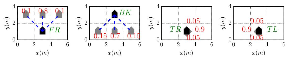 Figure 7
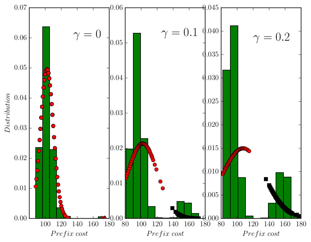 Figure 8
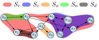 Figure 9
 Figure 10
 Figure 11
 Figure 12
 Figure 13
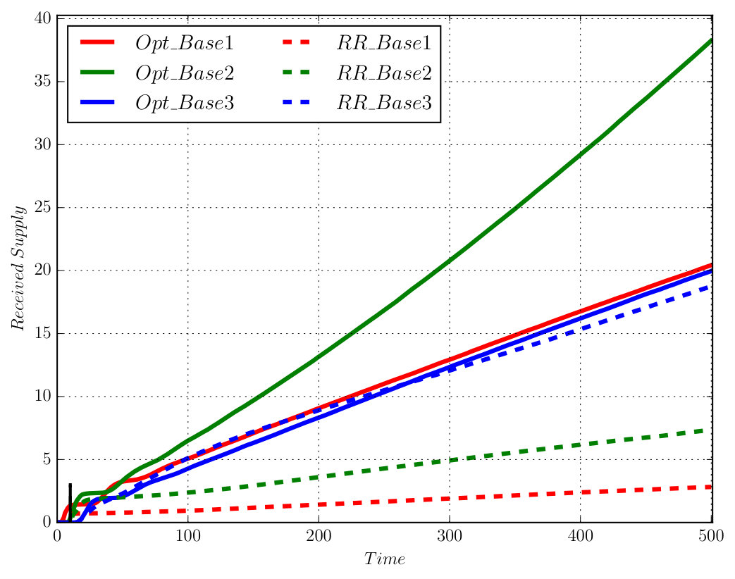 Figure 14
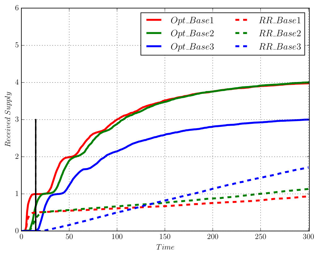 Figure 15
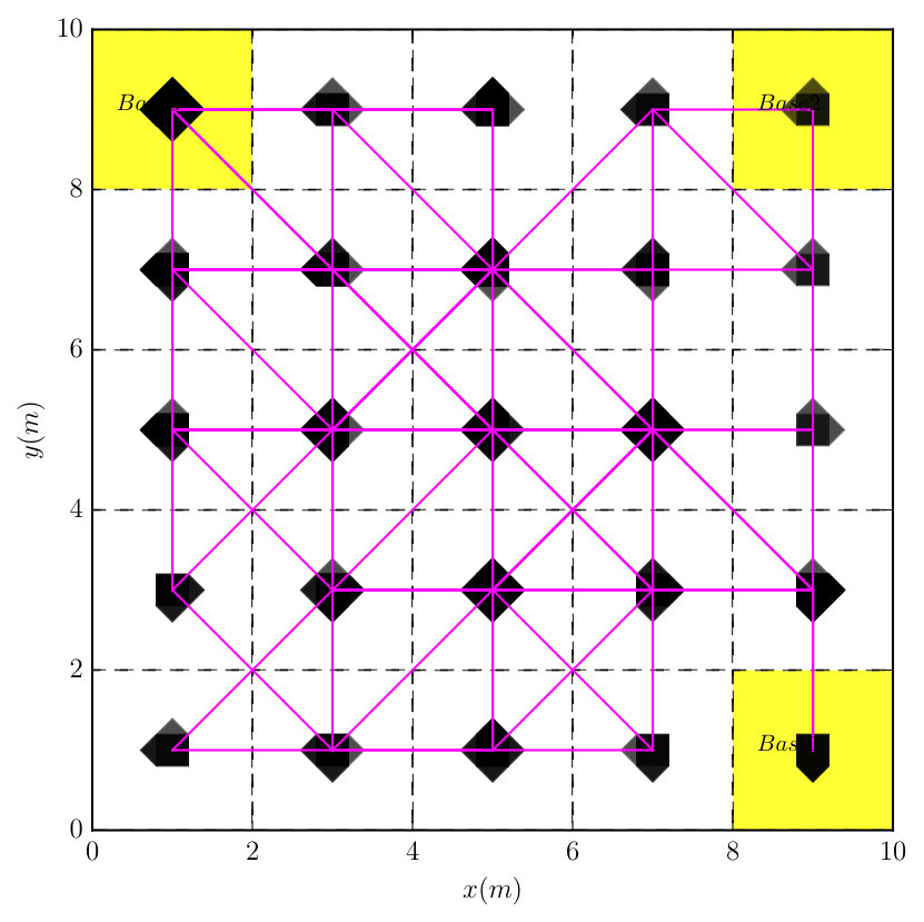 Figure 16
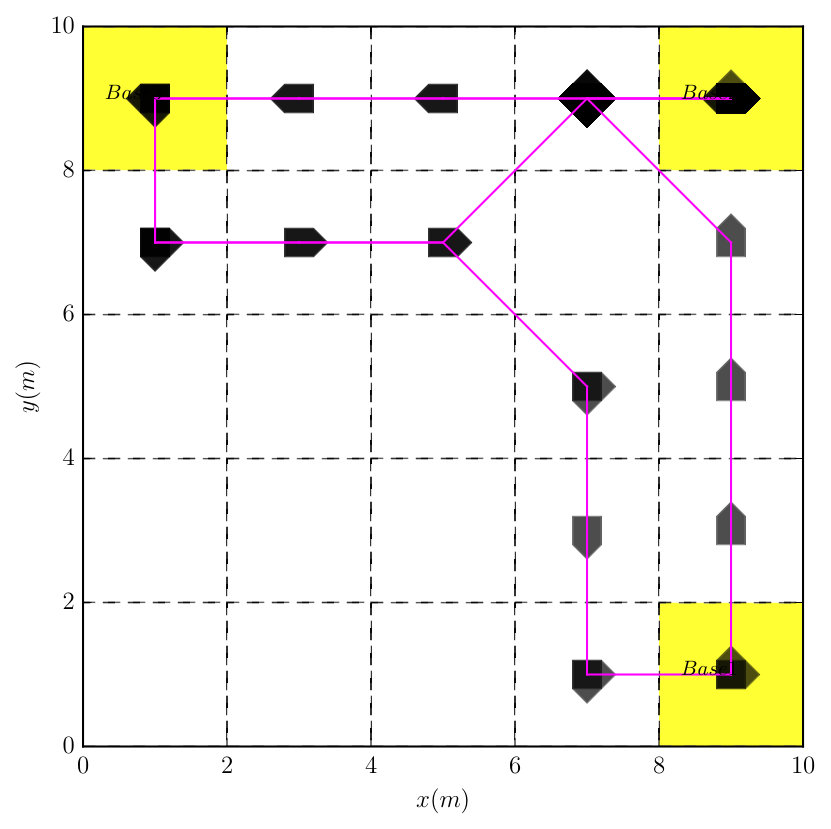 Figure 17
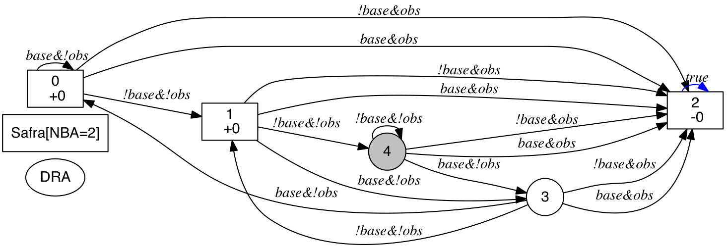 Figure 18
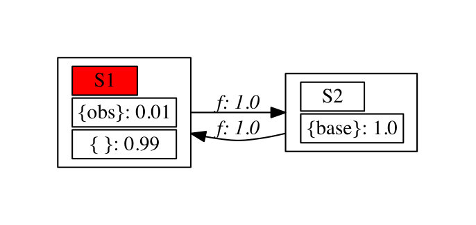 Figure 19
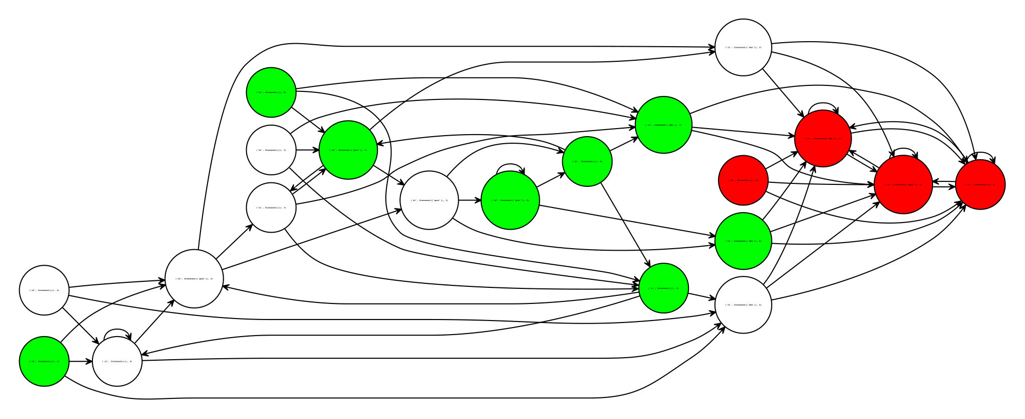 Figure 20
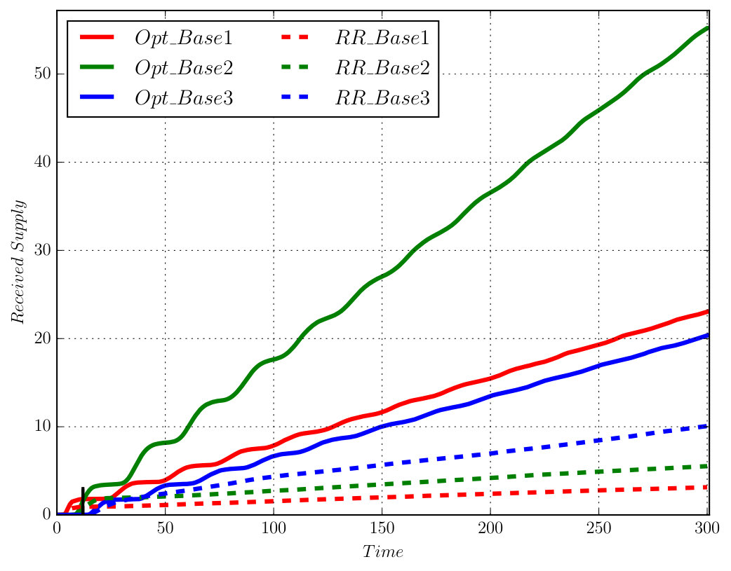 Figure 21
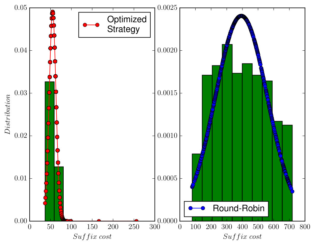 Figure 22
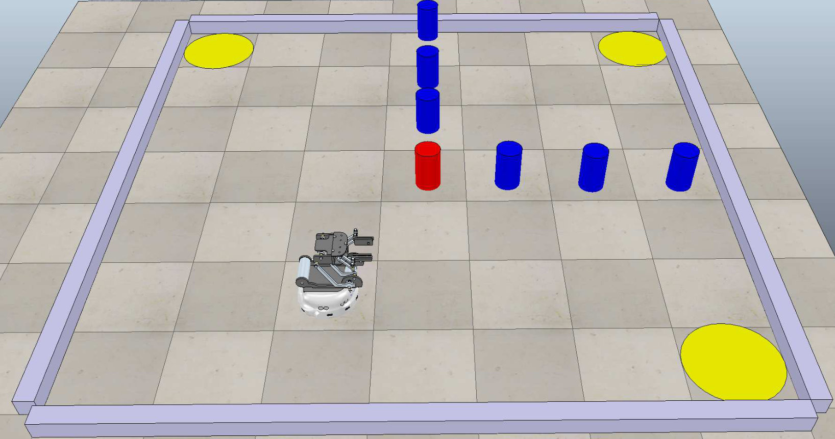 Figure 23
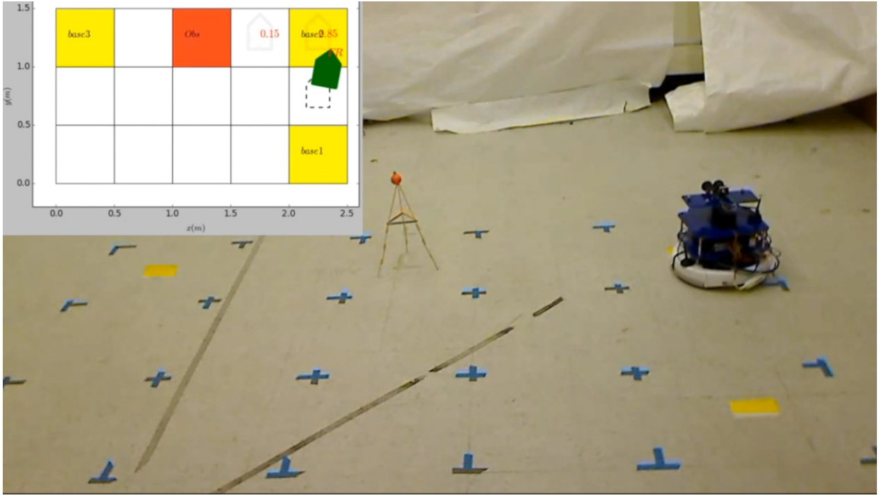 Figure 24
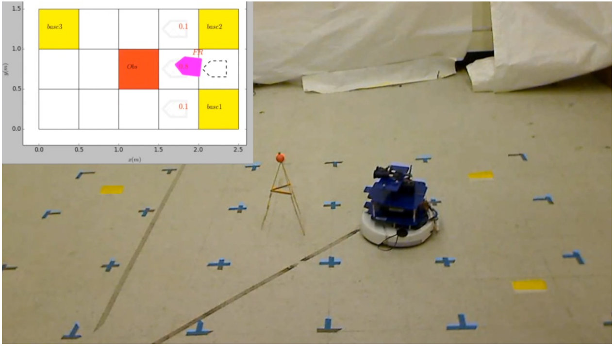 Figure 25
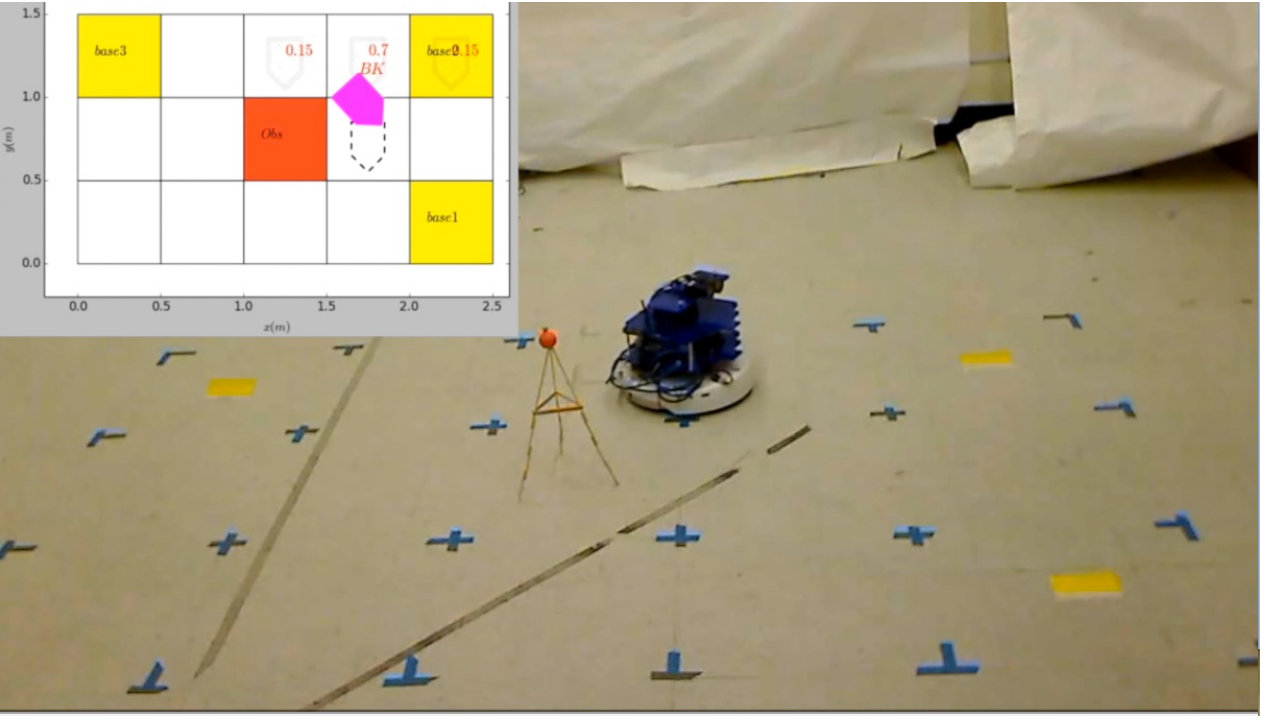 Figure 26
| Total Cost | Failure | Success | Unfinished | |
|---|---|---|---|---|
| 0 | 132.2 | 0 | 910 | 90 |
| 0.1 | 118.1 | 99 | 872 | 29 |
| 0.2 | 110.5 | 219 | 770 | 11 |
| 0.3 | 104.6 | 308 | 692 | 0 |
| 0.4 | 98.3 | 417 | 583 | 0 |
| AMECs | via (13) | |||||||
|---|---|---|---|---|---|---|---|---|
| Size | Time [] | Size | Time [] | Size | Time [] | Size of (8) | Size of (11) | Time to solve (13) [] |
| (100, 816) | 0.13 | (4.2e3, 4.1e4) | 16.3 | 1.2e3 | 4.15 | (443, 2.0e3, 8.3e3) | (1.2e3, 4.9e3, 2.1e4) | 0.21 |
| (324, 2.8e3) | 1.69 | (1.1e4, 1.0e5) | 41.2 | 3.6e3 | 29.4 | (1.3e3, 6.3e3, 2.2e4) | (3.6e3, 1.7e4, 5.9e4) | 0.72 |
| (900, 8.4e3) | 24.2 | (2.9e4, 2.8e5) | 106.8 | 1.0e4 | 337.1 | (3.6e3, 1.7e4, 6.0e4) | (9.9e3, 4.8e4, 1.6e5) | 16.74 |
| (1.4e3, 1.3e4) | 88.7 | (4.7e4, 4.5e5) | 391.7 | 1.6e4 | 1.1e3 | (5.8e3, 2.8e4, 9.7e4) | (1.5e4, 7.7e4, 2.6e5) | 20.81 |
| (2.5e3, 2.4e4) | 326.9 | (8.1e4, 7.8e5) | 290.1 | 2.7e4 | 4.8e3 | (1.0e4, 4.9e4, 1.6e5) | (2.7e4, 1.3e5, 4.5e5) | 15.74 |
| (3.3e3, 3.2e4) | 558.3 | (1.0e5, 1.1e6) | 380.1 | 3.7e4 | 9.4e3 | (1.3e4, 6.6e4, 2.2e5) | (3.7e4, 1.8e5, 6.1e5) | 32.04 |
| Prefix Cost | Suffix Cost | Balanced Cost by (13) | ||
| Total | Mean | |||
| 0 | 180.7 | 66.1 | 2.524 | 66.1 |
| 0.2 | 62.4 | 67.1 | 2.533 | 65.2 |
| 0.4 | 50.5 | 72.9 | 2.551 | 64.1 |
| 0.6 | 49.8 | 73.5 | 2.552 | 59.3 |
| 0.8 | 49.5 | 74.3 | 2.554 | 54.4 |
| 1.0 | 49.5 | 246.7 | 2.817 | 49.5 |
| Failure | Pre. Success | Suf. Success | |||
|---|---|---|---|---|---|
| 0.1 | 0.05 | 106 | 894 | 852 | |
| 0.2 | 0.05 | 169 | 831 | 785 | |
| 0.3 | 0.05 | 318 | 682 | 650 | |
| 0.4 | 0.05 | 409 | 591 | 549 | |
| 0.1 | 0.85 | 888 | 901 | 117 | |
| 0.1 | 0.98 | 997 | 903 | 4 |
| ASCCs | via (14) | |||||||
|---|---|---|---|---|---|---|---|---|
| Size | Time [] | Size | Time [] | Size | Time [] | Size of (8) | Size of (12) | Time to solve (14) [] |
| (100, 816) | 0.13 | (1.0e3, 1.1e4) | 0.9 | 3.1e2 | 0.66 | (202, 920, 3.4e3) | (301, 1.4e3, 4.9e3) | 0.45 |
| (324, 2.8e3) | 1.57 | (2.9e3, 3.1e4) | 3.39 | 9.8e2 | 1.84 | (6.5e2, 3.1e3, 1.1e4) | (9.7e2, 4.7e3, 1.6e4) | 2.41 |
| (900, 8.4e3) | 23.9 | (7.7e3, 7.9e4) | 7.04 | 2.7e3 | 5.09 | (1.8e3, 8.7e3, 3.0e4) | (2.7e3, 1.3e4, 4.5e4) | 9.89 |
| (1.4e3, 1.3e4) | 92.2 | (1.2e4, 1.2e5) | 9.78 | 4.3e3 | 8.41 | (2.9e3, 1.4e4, 4.9e4) | (4.3e3, 2.1e4, 7.2e4) | 22.94 |
| (2.5e3, 2.4e4) | 322.1 | (2.1e4, 2.1e5) | 20.1 | 7.5e3 | 17.1 | (5.1e3, 2.5e4, 8.5e4) | (7.5e3, 3.7e4, 1.3e5) | 83.33 |
| (3.3e3, 3.2e4) | 625.2 | (2.8e4, 2.9e5) | 23.1 | 1.0e4 | 19.6 | (6.7e3, 3.3e4, 1.1e5) | (1.0e4, 4.9e4, 1.7e5) | 145.8 |
Peer Reviews
No public reviews on file for this paper yet. If you reviewed it on a platform where reviews are public (OpenReview, ICLR, NeurIPS, ICML), you can paste yours below so the community can read it here.
Code & Models
Videos
No videos yet. Explain this paper in a talk, walkthrough, or lecture? Add one.
Taxonomy
TopicsRobotic Path Planning Algorithms · Formal Methods in Verification · Reinforcement Learning in Robotics
Probabilistic Motion Planning under Temporal Tasks
and Soft Constraints
Meng Guo, and Michael M. Zavlanos The authors are with the Department of Mechanical Engineering and Materials Science, Duke University, Durham, NC 27708 USA. Emails: meng.guo, [email protected]. This work is supported in part by NSF under grant IIS #1302283.
Abstract
This paper studies motion planning of a mobile robot under uncertainty. The control objective is to synthesize a finite-memory control policy, such that a high-level task specified as a Linear Temporal Logic (LTL) formula is satisfied with a desired high probability. Uncertainty is considered in the workspace properties, robot actions, and task outcomes, giving rise to a Markov Decision Process (MDP) that models the proposed system. Different from most existing methods, we consider cost optimization both in the prefix and suffix of the system trajectory. We also analyze the potential trade-off between reducing the mean total cost and maximizing the probability that the task is satisfied. The proposed solution is based on formulating two coupled Linear Programs, for the prefix and suffix, respectively, and combining them into a multi-objective optimization problem, which provides provable guarantees on the probabilistic satisfiability and the total cost optimality. We show that our method outperforms relevant approaches that employ Round-Robin policies in the trajectory suffix. Furthermore, we propose a new control synthesis algorithm to minimize the frequency of reaching a bad state when the probability of satisfying the tasks is zero, in which case most existing methods return no solution. We validate the above schemes via both numerical simulations and experimental studies.
Index Terms:
Markov Decision Process, Linear Temporal Logic, Chance Constrained Optimization, Motion Planning.
I Introduction
In this paper we study the problem of robot motion planning under uncertainty and temporal task specifications. We consider uncertainty in the workspace properties, robot motion and actions, and outcome of task executions, which gives rise to a Markov Decision Process (MDP) to model the proposed system. MDPs have been used extensively to model motion and sensing uncertainty in robotics [1, 2] and then solve decision making problems that optimize a given control objective. The most common objective is to reach a goal state from an initial state while minimizing the cost. The resulting solution is a policy that maps states to actions [2]. On the other hand, Linear Temporal Logic (LTL) provides a formal language to describe complex high-level tasks beyond the classic start-to-goal navigation. A LTL task formula is usually specified with respect to an abstraction of the robot motion within the allowed workspace [3], modeled by a deterministic finite transition system (FTS). Then a high-level discrete plan is found using off-the-shelf model-checking algorithms [4], which is then executed through low-level continuous controllers [3, 5]. This framework is extended to allow for both robot motion and actions in the task specification [6] and partially-known or dynamic workspaces in [7, 8].
Recently, there have been many efforts to address the problem of synthesizing a control policy for a MDP that satisfies high-level temporal tasks specified in various formal languages. Different classes of Probabilistic Computation Tree Logic (PCTL) formulas have been studied in [9] for abstraction and verification over Interval-valued Markov Chains. The work in [10] proposes a control policy for a mobile robot that maximizes the probability of satisfying a bounded linear temporal logic (BLTL) formula. Syntactical co-safe LTL formulas (sc-LTL) are considered in [11] for a deterministic robot that co-exists with other robots whose behavior is modeled as a MDP. A FTS with time-varying rewards is controlled to satisfy a LTL formula and maximize the accumulated reward in [12]. A robust control policy for MDPs with uncertain transition probabilities is proposed in [8]. A verification toolbox is provided in [13] for probabilistic discrete-time or continuous-time Markov Chain (MC), under a wide variety of quantitative properties expressed in PCTL, LTL, CTL, and so on.
In this work, we study motion planning of a mobile robot under uncertainty in both robot motion and workspace properties. The goal is to synthesize a finite-memory control policy that generates robot trajectories that satisfy a high-level LTL task formula with desired high probability. At the same time, we optimize the total cost both in the prefix and suffix parts of the system trajectories. Our proposed approach is based on solving two coupled Linear Programs, one for the prefix and one for the suffix, over the occupancy measures of the product automaton introduced in [14]. Moreover, we explore cases where the probability of satisfying the LTL tasks is zero, so that an Accepting End Component (AEC) does not exist in the MDP, where most relevant work returns no solutions. To address such situations, we treat satisfaction of the tasks as soft constraints and propose a relaxed suffix plan that minimizes the frequency with which the system enters bad states that violate the task specifications. We show that our approach outperforms the widely-used Round-Robin policy, via both numerical simulations and experimental studies. We also compare our proposed method with the widely-used probabilistic model-checking tool PRISM [13].
Our work is related to literature on (i) policy synthesis for MDPs under multiple objectives; (ii) cost optimization within AECs in MDPs; and (iii) infeasible temporal tasks. We discuss below this literature and highlight our contributions.
Since we consider both temporal tasks and total-cost criteria over MDPs, this work is closely related to policy synthesis of MDPs under multiple objectives. The work in [14] proposes a framework with provable correctness to synthesize a control policy for MDPs under multiple constrained total-cost criteria. A survey on multi-objective decision-making for MDPs can be found in [15]. On the other hand, verification of MDPs under multiple high-level tasks is addressed in [16], where the probability of satisfying each subtask is lower-bounded by a given value. Moreover, a quantitative multi-objective verification scheme is proposed in [17, 18] for numerical queries over probabilistic reward predicates.
On the other hand, the seminal works [19, 20] consider MDPs with multi-dimensional weights under multi-percentile queries that may be conflicting. However, most of the above work does not address cost optimization over the suffix of the system trajectory within the AECs, neither does it address the case where no AECs can be found in the product automaton, which are the main contributions here.
The satisfaction of a LTL formula is associated with reaching the corresponding AECs. In particular, in [4, Chapter 10], a value iteration method is used to solve the maximal reachability problem towards the AECs to obtain a policy for the plan prefix. For planning within the AECs, [21, 17, 4] adopt the Round-Robin policy, which guarantees only correctness but not optimality. Optimal policies for the plan suffix that keeps the system within the AECs have been proposed in [22, 23, 24, 25]. Specifically, in [22] the expected cost of satisfying instances of a desired property is minimized, while in [23] the minimal bottleneck cost is considered. Both approaches in [22, 23] require particular types of LTL formulas (such as “always eventually”). The work in [24, 26] considers MDPs with -regular specifications and quantitative resource constraints within the AECs. The work in [25] investigates the Pareto cost of a human-in-the-loop MDP measured by a given discounted cost function. Compared to this literature, the multi-objective optimization problem that we formulate to solve the control synthesis problem allows us to explicitly characterize the trade-off between prefix and suffix optimality. We then extend this methodology to the case where no AECs can be found.
Most aforementioned work [19, 20, 27, 4, 17, 21, 22] relies on the assumption that the product automaton contains at least one AEC. However, in many situations this assumption does not hold so that the probability of satisfying the task under any policy is zero. In this case, it is still important to identify those policies that minimize the frequency with which the system will reach the bad states that violate the task specifications. Consequently, it is desirable to synthesize a policy with certain risk guarantees even when soft LTL tasks are considered that are only partially-feasible. To the best of our knowledge, there is no work on control synthesis for infeasible soft LTL task formulas defined on MDPs, especially when an AEC can not be found in the resulting product automaton. For deterministic transition systems, a framework for robot motion planning in partially-known workspaces is proposed in [7] that can handle soft LTL task formulas whose satisfiability is improved over time; a least-violating control strategy is synthesized in [28] for a set of LTL safety rules. In the case of MDPs, a relevant formulation is considered in [29] where a MDP is controlled to satisfy an -regular formula. A policy is proposed to ensure that the MDP enters a failure state relatively late in the prefix. However, a multi-objective criterion of the control policy, especially in the plan suffix, is not considered there. Also, recent work in [30] proposes an approach to increase the satisfaction probability by modifying the task formula which, however, only considers co-safe LTL formulas without cost optimization constraints.
In summary, the main contribution of this work is three-fold: (i) a framework that optimizes the total cost both in the plan prefix and suffix, while ensuring that the tasks are satisfied with a desired high probability; (ii) a new algorithm to synthesize the control policies that have a high probability of satisfying the task over long time intervals, for cases where an AEC does not exist; and (iii) a new method that allows the system to recover from bad states and continue the task.
The rest of the paper is organized as follows. Section II introduces necessary preliminaries. In Section III, we formalizes the considered problem. Section IV presents our solution in details, which includes four major parts. Section V demonstrates the feasibility of the results by numerical simulations. Section VI contains the experimental results. We conclude and discuss about future directions in Section VII.
II Preliminaries
II-A Transient MDP
A Markov Decision Process (MDP) is defined as a 6-tuple , where is the finite state space; is the finite control action space (with a slight abuse of notation, also denotes the set of control actions allowed at state ); is the set of possible state-action pairs; is the transition probability function so that is the transition probability from state to state via control action and , ; that is the cost of performing action at state ; and is the initial state. Denote by , .
The above MDP evolves by taking an action associated with every state . Denote by the past run that is a sequence of previous states and actions up to time . As defined in [2], a control policy is a sequence of decision rules at time . A control policy is stationary if , , where can be randomized so that or deterministic so that , . On the other hand, a policy is history dependent or finite-memory if , where is the past history until time .
II-B End Components
A sub-MDP of is a pair where and such that (i) , , ; (ii) , and . An End Component (EC) of is a sub-MDP such that the digraph induced by is strongly connected. An end component is called maximal if there is no other end component such that , and , . The set of Maximal End Components (MECs) of a MDP is finite and can be uniquely determined. The analysis of MECs would include each EC as a special case. We refer the readers to Definitions 10.116, 10.117 and 10.124 of [4] for details. Moreover, an Accepting MEC (AMEC) is an end component that satisfies certain accepting conditions such as the Streett and Robin conditions, which will be defined in the sequel. On the other hand, a Strongly Connected Component (SCC) of the digraph induced by is a set of states so that there exists a path in each direction between any pair of states in . Similarly, an Accepting SCC (ASCC) is a SCC that satisfies certain accepting conditions. Note that the main difference between a MEC and a SCC is that the SCC does not restrict the set of actions that can be taken at each state . In other words, there might be paths that start from any state within the SCC and end at states outside the SCC.
II-C LTL and DRA
The ingredients of a Linear Temporal Logic (LTL) formula are a set of atomic propositions and several Boolean and temporal operators. Atomic propositions are Boolean variables that can be either true or false. A LTL formula is specified according to the syntax [4]: where , , (next), U (until) and . For brevity, we omit the derivations of other operators like (always), (eventually), (implication). The semantics of LTL is defined over the set of infinite words over . Intuitively, is satisfied on a word if it holds at , i.e., if . Formula holds true if is satisfied on the word suffix that begins in the next position , whereas states that has to be true until becomes true. Finally, and are true if holds on eventually and always, respectively. We refer the readers to Chapter 5 of [4] for the full definition.
The set of words that satisfy a LTL formula over can be captured through a Deterministic Rabin Automaton (DRA) [4], defined as , where is a set of states; is the alphabet; is a transition relation; is the initial state; and is a set of accepting pairs, i.e., where , . An infinite run of is accepting if there exists at least one pair such that , it holds and , , where stands for “existing infinitely many”. Namely, this run should intersect with finitely many times while with infinitely many times. There are translation tools [31] to obtain given , which requires the process of translating firstly the LTL formula to the associated Nondeterministic Büchi Automaton (NBA), and then to the DRA with complexity , where is the length of . Our implementation of the Python interface for [31] can be found in [32]. Note that [31] allows for different levels of automata simplifications to be made regarding the size of , and a simplified automation may result in loss of optimality.
III Problem Formulation
III-A Mathematical Model
In order to model uncertainty in both the robot motion and the workspace properties, we extend the definition of a MDP from Section II-A to include probabilistic labels, as the probabilistically-labeled MDP:
[TABLE]
where is a set of atomic propositions that capture the properties of interest in the workspace; contains the set of property subsets that can be true at each state; and specifies the associated probability. Particularly, denotes the probability that state satisfies the set of propositions . Note that , . Moreover, contains the initial state and the initial label , while the rest of the notations in (1) are the same as defined in Section II-A. The probabilistic labeling function provides a way to consider time-varying and dynamic workspace properties. Moreover, there is a LTL task formula specified over the same set of atomic propositions , as the desired behavior of . We assume that the MDP in (1) is fully-observable due to the following assumption.
Assumption 1**.**
At any stage , the current robot state and its label are fully-observable.
While the robot is moving within the workspace, it is capable of sensing an actual property and determine the label of the state it is located at. At stage , the robot’s past path is given by , the past sequence of observed labels is given by and the past sequence of control actions is . It holds that and , . These three sequences can be composed into the complete past run . Denote by , and the set of all possible past sequences of states, labels, and runs up to stage . We set for infinite sequences.
Definition 1**.**
The mean total cost [33, 2] of an infinite robot run of is defined as
[TABLE]
where .
As discussed in [33, 24, 20, 2], the above mean total cost is called the mean-payoff function (or limit-average), where the “” operator is needed as the limit-average might not exist for some runs, see [33, 24, 34].
Our goal is to find a finite-memory policy for , denoted by . The control policy at stage is given by , where is the past run , . Denote by the set of all such policies. Given a control policy , the probability measure on the smallest -algebra, over all possible infinite sequences that contain , is the unique measure [4] by
[TABLE]
where is defined as the probability of choosing action given the past run . Then we define the probability of satisfying under policy by:
[TABLE]
where the satisfaction relation “” is introduced in Section II-C, given an infinite word and a LTL formula. Accordingly, the risk is defined as the probability that the task formula is not satisfied by under the policy , namely, .
Problem 1**.**
Given the labeled MDP defined in (1) and the task specification , our goal is to sovle:
[TABLE]
where is a pre-defined parameter as the allowed risk; the optimal policy minimizes the mean total cost and ensures that the risk of violating remains bounded by .
Note that the traditional definition of un-discounted expected total cost over an infinite run from [14, 2] is not used here, as it is infinite except for the special case of transient MDPs defined in Section II-A. However, in this work, the model is not restricted to be transient. Moreover, the discounted total cost in [2] is not used here either due to two reasons: first, it is not obvious how to choose the discount factor for various control tasks [25]; and second, we are more interested in optimizing the repetitive long-term behavior of the system, rather than the short-term one [20]. In-depth discussions on the optimization of infinite-horizon un-discounted or discounted total-cost criteria over MDPs with or without constraints can be found in [2].
Remark 1**.**
Different from the maximal reachability problem addressed in [4, 21], a deterministic policy would not suffice here. Instead, randomization is required due to the mean total-cost criterion and the risk constraint, similar to [14].
IV Solution
This section contains the three major parts of the proposed solution: (i) the construction of the product automaton and its AMECs; (ii) the algorithms to synthesize the optimal plan prefix and suffix, for both cases where the AMECs exist or not; (iii) the complete policy, and the online execution algorithm.
IV-A Product Automaton and AMECs
To begin with, we construct the DRA associated with the LTL task formula via the translation tools [31, 32]. Let it be , where the notations are defined in Section II-C. Then we construct a product automaton between the robot model and the DRA .
Definition 2**.**
Denote by the product as a 7-tuple:
[TABLE]
where: the state is so that , , and ; the action set is the same as in (1) and , ; ; the transition probability is so that
[TABLE]
where (i) ; (ii) ; and (iii) ; the cost function is so that c_{E}\big{(}\langle x,l,q\rangle,\,u\big{)}=c_{D}(x,u), \forall\big{(}\langle x,l,q\rangle,\,u\big{)}\in E. Namely, the label should fulfill the transition condition from to in ; the single initial state is ; the accepting pairs are defined as , where and , .
The product computes the intersection between all traces of and all words that are accepted by , to find all admissible robot behaviors that satisfy the task . It combines the uncertainty in robot motion and the workspace model by including both and in the states. The Rabin accepting condition of is defined as follows: An infinite path of is accepting if for at least one pair it holds that intersects with finitely often while with infinitely often. To transform this condition into equivalent graph properties, we need to compute the AMECs of associated with its accepting pairs . Detailed definition of MECs is given in Section II-B.
In order to find the complete set of AMECs of , for each pair , perform the following steps:
(i) Build the MDP , where is the set of states with and a trap state; is the set of actions where is a pseudo action; is the set of transitions with the associated probability which are defined by three cases: (a) for the transitions within it holds that and , where ; (b) for the transitions from to outside it holds that and , where ; and (c) the trap state is included in a self-loop such that and . Simply speaking, all transitions from inside to outside are transformed to transitions to the trap state .
(ii) Determine all MECs of above via Algorithm 47 in [4], which is based on splitting the strongly connected components (SCCs) of until the conditions of being an end component are fulfilled. Our implementation for this algorithm can be found in [32]. Denote by the set of MECs, where and , . Note that , .
(iii) Find that is accepting, i.e., it satisfies and . Save the AMECs in . Since is computed for each , we denote by the complete set of AMECs of .
Remark 2**.**
A single state with a self-transition can be a MEC with a proper action set. Therefore, there exists at most MECs within , . Thus Step (ii) above has complexity , as shown in Lemma 10.126 of [4], while Steps (i) and (iii) have complexity linear with .
IV-B Plan Prefix and Suffix Synthesis
Given the complete set of AMECs of , in this section we show how to synthesize the control policy to drive the system towards and furthermore remain inside while satisfying the accepting condition. As mentioned in Section I, most related work [21, 4, 16, 17] focuses on maximizing the probability of reaching the union of AMECs, i.e., , where dynamic programming techniques, such as value or policy iteration, can be applied to obtain the optimal policy. Furthermore, once the system enters any AMEC, e.g., , it has probability of staying within by following (see Lemma 10.119 of [4]). The Round-Robin policy is adopted in [21, 17, 4] that ensures all states in (including its nonempty intersection with ) are visited infinitely often. As a result, the task is satisfied by under this policy with the maximal probability.
The above solutions may suffice for verification problems that do not optimize cost or for tasks with trivial accepting conditions. However, for the purposes of plan synthesis and for general tasks, it is of practical interest to simultaneously satisfy the probability of reaching all the AMECs as well as optimize the mean cost of staying within any AMEC and fulfilling the accepting condition. Moreover, when no AECs can be found, instead of simply reporting failure, it is important to obtain a relaxed policy that guarantees high probability of satisfying the task over long time intervals thus minimizing the frequency of encountering bad events. In what follows we present a policy synthesis algorithm that consists of four parts:
- •
the plan prefix that drives the system from the initial state to all AMECs, while minimizing the expected cost and respecting the risk constraint; see Section IV-B1;
- •
the plan suffix that keeps the system within the AMEC it has reached, while satisfying the accepting condition and optimizing the expected suffix cost; see Section IV-B2;
- •
the relaxed prefix and suffix plans for the case where no AECs of can be found; see Section IV-B3; and
- •
the complete finite-memory policy for the original MDP ; see Section IV-C1.
Before stating the solution, we introduce a partition of given the initial state and the set of AMECs . Let be the set of states within that can be reached from , which can be derived via a simple graph search in .
Definition 3**.**
Given and , is partitioned as , where is the set of states that can not be reached from ; is the union of all goal states in , i.e., ; can be reached from but can not reach any state in ; and .
The set can be derived through a simple graph search, e.g., by reversing the directed graph associated with , finding all reachable nodes of any state within each (as any AMEC is strongly connected) and finally computing its cross intersection with ; see [32] for implementation details. Roughly speaking, is the set of states related to the plan prefix, is the set of goal states related to the plan suffix, and is set of bad states to be avoided during the prefix. Since contains the states that can not be reached from , it is neglected hereafter for the purpose of plan synthesis.
Example 1**.**
This example illustrates the partition in Definition 3. Consider the toy product automaton in Figure 2. For state , the set of reachable states is , the set of unreachable states is , the states within an AMEC are and another AMEC , thus , the states that can be reached from but can not reach are , and the states that can reach outside are .
IV-B1 Plan Prefix
Similar to [17, 18], we first construct a modified sub-MDP of as , where the set of states is given by with being defined in Definition 3. The set of actions is given by where is a self-loop action. The set of transitions is the subset of associated with . Moreover, the transition probability is defined by (i) , where and ; and (ii) , . Finally, the cost function is defined by (i) , and ; and (ii) , .
Then, we find a policy for such that, starting from , it can reach the set of goal states with a probability larger than , while at the same time minimizing the expected total cost. Formally, consider the problem below:
Problem 2**.**
Given the sub-MDP , compute an optimal stationary prefix policy that solves the problem
[TABLE]
where is a run of , is the set of all stationary policies, the objective function is the expected total cost, is the probability of reaching from the initial state , under the policy ; and is from (4).
Note that the objective function in (7) is well-defined and finite due to the fact that is transient with respect to , and is equal to the expected total cost of reaching since the cost of staying within is zero. We omit the proof that is transient here and refer the interested readers to [2, 14]. Our proposed solution to Problem 2 is based on transforming it into a constrained optimization problems for MDPs, which can be then solved using linear programming. The approach is inspired by [16, 17, 14]. Particularly, denote by the expected number of times over the infinite horizon that the system is at state and action is taken, and , which are often referred to as occupancy measures [14] as it holds , where the probability is conditioned on a policy and the initial state . Note that an occupancy measure is a sum of probabilities, but not a probability itself. Consider the linear program:
[TABLE]
where , the indicator function if and , otherwise. Denote by the objective function associated with . Let the solution of (8) be . Then the optimal stationary policy for the plan prefix, denoted by , can be derived as follows: the probability of choosing action at state equals to if ; otherwise, the action at can be chosen randomly, .
Lemma 1**.**
Given an optimal solution of (8), the associated policy ensures that .
Proof.
First, is finite and well-defined since is transient with respect to ,. The second part of the proof is similar to Lemma 3.3 of [16]. The summation is the expected number of times that transitions from any state in into for the first time, under policy from the initial state . Since the system remains within once it enters , the summation equals the probability of eventually reaching the set , which is lower-bounded by . This completes the proof. ∎
Example 2**.**
This example illustrates the important role of in the trade-off between reducing the expected total cost and minimizing the risk in Problem 2. Consider the unicycle robot with action primitives illustrated in Figure 1 and defined in Section V. The robot moves within partitioned cells as shown in Figure 3, where the red cell has probability to be occupied by an obstacle. Consider the task: , i.e., to reach the yellow base without crossing any obstacle. In what follows, we solve (8) under risk factors and to derive two different optimal policies. Figure 3 shows a shorter trajectory with lower expected total cost of about when a larger risk is allowed, compared with the right trajectory that avoids completely colliding with the obstacle, but with a much higher total cost of about .
IV-B2 Plan Suffix with AMECs
In this section, we present an algorithm to synthesize the plan suffix that minimizes the mean total cost within the AMECs, while ensuring that the system trajectory satisfies the accepting condition of . Note that the plan prefix from the previous section guarantees that the system enters from with probability higher than . Recall also that . Thus it is possible that the system enters any set within . For this reason, we propose to treat each AMEC separately, as each is associated with different and thus a different accepting condition for . Specifically, consider any AMEC and let , which is nonempty by the definition of an AMEC.
Once the system enters any AMEC, most related work [21, 17, 4] adopts the Round-Robin policy defined below:
Definition 4**.**
For each state , create any ordered sequence of actions from , denoted by and its infinite repetition by . Then at any stage , whenever the system reaches , the Round-Robin policy instructs the system to take the next action in , starting from the first action in .
Namely, once the system enters , the Round-Robin policy iterates over the allowed actions for each state, which in-turn ensures that all states in (which include ) are visited infinitely often. Detailed can be found in Lemma 10.119 in [4].
Definition 5**.**
An accepting cyclic path of , associated with and , is a finite path that starts from any state and ends in any state , while remaining within .
Note that an accepting cyclic path does not necessarily start and end at the same state in . Furthermore, we can define the mean cyclic cost of under a stationary policy.
Definition 6**.**
The total cost of a cyclic path is defined as
[TABLE]
where is the length of the path and . Then its mean total cost is defined as .
Problem 3**.**
Find a stationary suffix policy for within that minimizes the mean cyclic cost
[TABLE]
where is the set of all accepting cyclic paths associated with the AMEC .
Inspired by [33, 24, 20], we formulate a Linear Program to solve the mean-payoff optimization problem. First, we construct a modified sub-MDP of over by splitting into two virtual copies: which only has incoming transitions into and that has only outgoing transitions from . Formally, we define , where the set of states is with and the virtual copies of . The set of control actions is , where is a self-loop action. The set of state-action pairs is defined by (i) , and ; (ii) , ; and (iii) , and . Moreover, is the initial distribution of all states in that can be reached by taking a transition from states in , defined by
[TABLE]
where are the variables of (8). Furthermore, the transition probability is defined in five cases below: (a) for transitions within , it holds that , , ; (b) for transitions originated from , it holds that , , and ; (c) for transitions into , it holds that , , and ; (d) for transitions from to , it holds that , and ; and (e) for transitions within , , . Lastly, the cost function satisfies , , , and , .
Remark 3**.**
The initial distribution of indicates how likely it is that the system controlled by the plan prefix will enter the AMEC via each state inside .
Let also and denote by the long-run frequency with which the system is at state and the action is applied, and . Then, we can formulate the following linear program to solve Problem 3:
[TABLE]
where , the first constraint ensures that is eventually reached, while the second constraint balances the incoming and outgoing flow at each state. Let its solution be . Then, the optimal stationary policy for the plan suffix, denoted by , can be derived as follows: the probability of choosing action at state equals to if ; otherwise the action at is chosen randomly, . Note that , and . Namely, once the system reaches any state , the control policy at will be the control policy for , according to the solution of (11).
Remark 4**.**
The initial distribution is derived from (8), instead of being arbitrarily set as in [25]; Moreover, (11b) ensures that only is intersected infinitely often, instead of enforcing that all states in the set are visited infinitely often as in [25].
Lemma 2**.**
If (11) has a solution, then the plan suffix solves Problem 3 for the chosen AMEC .
Proof.
First, by Definition 5, the objective in (11) equals the mean cyclic cost of all accepting cyclic paths for . Moreover, by the definition of an AMEC, any path remains within by choosing only actions within at each state . ∎
Lemma 3**.**
Let be the set of all accepting runs of that enter after a finite number of steps. If is generated under , then satisfies the accepting condition of . Moreover, the mean total cost in (2) equals the mean cyclic cost in (10), i.e., .
Proof.
By (11), any system trajectory of under contains infinite occurrences of accepting cyclic paths. Since any accepting cyclic path starts from and ends in (which is finite), intersects with infinitely often. Moreover, since any accepting cyclic path remains within , remains within for all time after entering . In other words, intersects with a finite number of times before entering and then intersects infinitely often after entering , which satisfies the Rabin accepting condition of . To show the second part, notice that the product under evolves as a Markov chain and the set of all accepting cyclic paths within has a stationary distribution. By viewing any accepting run as the concatenation of an infinite number of cyclic paths, the mean total cost of defined in (4) over an infinite time horizon equals the mean cyclic cost in (10) of all cyclic paths contained in . This result is important in showing the equivalence between Problems 1 and 3 later in Theorem 6. ∎
Example 3**.**
This example illustrates the difference between the plan suffix obtained by (11) and the Round-Robin policy. Consider the same robot model from Example 2 and the partitioned workspace in Figure 4. The task is to surveil three base stations in the corners, i.e. . The plan prefix is derived by solving (8) but two different plan suffixes are used: one using (11) and the Round-Robin policy. Figure 4 shows the simulated trajectory under these two policies. It can be seen that the trajectory under the optimal plan suffix approximates the shortest route to cross all base stations, while the trajectory under the Round-Robin policy exhibits a rather random behavior.
IV-B3 Plan Synthesis when AECs do Not Exist
The synthesis algorithms proposed in Sections IV-B1 and IV-B2 rely on the assumption that the set of AMECs of is nonempty which, however, might not hold in many scenarios. In this case, most existing techniques proposed in [4, 17, 21, 22] can not be applied. In this section, we first provide a simple example where no AECs exist, and then propose an approach to synthesize a relaxed plan prefix and suffix.
Example 4**.**
This example provides a robot model and its task for which no AECs exist in the product automaton . Consider the MDP in Figure 5 that transitions between two states (, ) with probability using the action . Note that has only probability of being occupied by an obstacle and is the base station. The task is to surveil the base station while avoiding obstacles, i.e., . The associated DRA is shown in Figure 5. The resulting is shown in Figure 6, where the set of states to avoid in the suffix is in red and the set of states to intersect infinitely often in green. The reason that no AECs exist in is because by definition an AEC should include all successor states that are reachable by the single action . Then, starting from any green state in , the set of reachable states eventually intersect with the red states in .
When no AECs exist in , the probability of satisfying the task under any policy is zero. However, it is still important to identify those policies that ensure high probability of avoiding bad states over long time intervals. Consequently, we propose to use an accepting SCC (ASCC) of as the relaxed AMEC, due to the following lemma.
Lemma 4**.**
Assume there exists one infinite path of that is accepting. Then, there exists at least one SCC of that intersects with but not with , for at least one pair .
Proof.
As mentioned before, an infinite path of , denoted by , is accepting if for at least one pair it holds that intersects with all states in finitely often while with infinitely often. Since both and are finite, there exists a cyclic path of that contains at least one and does not contain any state within . By definition, this cyclic path is a SCC of that intersects with but not with . This completes the proof. ∎
Denote the set of SCCs in as , where . This set can derived using Tarjan’s algorithm [4, 32]. Moreover, denote by the set of SCCs that satisfy the accepting conditions associated with . Lemma 4 ensures that for at least one pair . Therefore, the union is not empty.
Now the union serves as the set of states the system should enter, starting from the initial state, and then remain inside any of the ASCC to satisfy the accepting condition. Again the first step is to formulate a Linear Program that minimizes the expected total cost of reaching from , while ensuring the risk is upper-bounded by the chosen . It can be done analogously as in (8) but over (which is omitted here). Denote the objective function by and its set of variables by and the associated relaxed plan prefix as . Same as in Section IV-B2, it is possible that the system under the policy can enter any ASCC in . Assume that the system enters . Different from an AMEC , the action set at each state of is not constrained. Thus, there is no guarantee that the system will stay within after entering it.
Therefore, the second step is to synthesize the relaxed plan suffix that keeps the system inside to satisfy the accepting condition with the maximal probability. Define the set , which is not empty for an ASCC . Then, an accepting cyclic path of associated with , and the cyclic cost associated with and can be defined similarly as in Definition 5. Formally, we consider the following problem:
Problem 4**.**
Find a control policy for that minimizes the mean cyclic cost associated with the ASCC : , where is the set of all accepting cyclic paths associated with and is defined as in Definition 6; while at the same time maximizing the probability that the cyclic paths stay within .
In Problem 4, the first objective of minimizing the mean cyclic cost corresponds to minimizing the mean total cost in (4) in Problem 1. The objective of maximizing the probability of the system staying within the ASCC corresponds to minimizing the frequency with which the system will reach the bad states that violate the task specifications. It constitutes a relaxation of the risk constraint (4) in Problem 1. To solve Problem 4, first we construct a modified MDP over , which is similar to in Section IV-B2. The set is split into two virtual copies: which only has incoming transitions and that has only outgoing transitions. Formally, we define , where the set of states is , with and the two virtual copies of , and is a virtual bad state. The set of control actions is given by , where is a self-loop action. The set of transition is which satisfies that (i) , and ; (ii) , ; and (iii) . Moreover, is the initial distribution of states in based on the transition from states in :
[TABLE]
where and are the variables solutions from the synthesis of the relaxed plan prefix, and . Furthermore, the transition probability is defined in seven cases below: (a) for transitions within , it holds that , , ; (b) for transitions originated from , it holds that , , and ; (c) for transitions into , it holds that , , and ; (d) for transitions from to , it holds that , and ; (e) for transitions into the bad state , it holds that , , and ; (f) each state within is included in a self-loop such that , ; (g) the bad state is included in a self-loop such that . Finally, the cost function is defined in two cases: (i) , , ; and (ii) , and .
Remark 5**.**
Note that contains all actions for each state in , compared with as allowed by the AMEC.
Let and . We can also show that above is transient. Then, to solve Problem 4, we rely on a technique proposed in [35] to deal with dead ends in Stochastic Shortest Path (SSP) problems. First we introduce a large positive penalty for reaching the dead state, denoted by . Then, we modify (11) as follows: denote by the long-run frequency with which the system is at state and the action is taken, and . We want to minimize the mean total cost of reaching from , while minimizing the probability of leaving . In particular, we consider the following optimization:
[TABLE]
where the notation , the variables satisfy that , , denotes the objective function as the summation of the mean cost of reaching and the expected penalty of reaching . The first constraint balances the incoming and outgoing flow at each state, while the second constraint ensures that are eventually reached. Let the optimal solution of (12) be . Then, the optimal stationary policy for the relaxed plan suffix, denoted by , can be derived as follows: for states in , the optimal policy is given by if ; otherwise the action at is chosen randomly, . Note that , and .
Lemma 5**.**
Under the relaxed plan suffix , the probability of reaching from while staying within over an infinite horizon, is lower bounded by , where .
Proof.
The proof is a simple inference from (12c). ∎
Remark 6**.**
A lower bound can be enforced on as in (8). However, this bound is hard to estimate and a large bound can yield the problem infeasible. In contrast, (12) always has a solution and is tunable by varying .
IV-C The Complete Policy
In this section, we present how to combine the stationary plan prefix and plan suffix of into the complete finite-memory policy of the original MDP . Furthermore, we show how to execute this finite-memory policy online.
IV-C1 Combining the Plan Prefix and Suffix
When AMECs of exist, we can combine the plan prefix synthesis and the plan suffix synthesis for each AMEC into one Linear Program:
[TABLE]
where and are defined in (8a) and (11a), respectively, the variables satisfy the constraints (8b)–(8d) and (11c), and the variables , where , satisfy the constraints (11c)–(11d) for the AMEC . The parameter captures the importance of minimizing the expected total cost to reach versus stay in . Note that the initial conditions in (11c) for each state in the suffix are expressed over the variables . In other words, the initial conditions of each AMEC are now optimized to solve the combined objective function (13). It can be solved via any Linear Programming solver, e.g., “Gurobi” [36] and “CPLEX”. Once the optimal solution and is obtained, the optimal plan prefix can be constructed as described in Section IV-B1 and the plan suffix as in Section IV-B2.
On the other hand, when no AECs of exist, as discussed in Section IV-B3, we can combine the relaxed plan prefix and suffix synthesis for each ASCC into one Linear Program:
[TABLE]
where and are defined in (8a) and (12a), respectively, the variables satisfy the constraints (8b)–(8d), and the variables , where , satisfy the constraints (12b)–(12d) for the ASCC . The parameter captures the importance of minimizing the expected total cost to reach versus stay in . Similar to the previous case, the initial conditions in (12b) for each state in the ASCCs are expressed over the variables . Thus the initial conditions are now optimized to solve the combined objective function (14). Again, it can be solved via any Linear Programming solver. Once the optimal and is obtained, the optimal relaxed plan prefix and relaxed plan suffix can be constructed as described in Section IV-B3.
Note that the size of both Linear Programs in (13) and (14) is linear with respect to the number of transitions in and can be solved in polynomial time [37]. Note also that the multi-objective costs introduced in (13) and (14) provide a balance between optimizing the plan prefix and suffix. Compared to only optimizing the plan suffix, i.e., for as required to solve Problems 3 and 4, increasing slightly the value of can lead to a significant decrease in the total cost of the plan prefix, without sacrificing much the optimality in the plan suffix.
Observe that the optimal policy derived above only includes the states within . Thus no policy is specified for the bad states in . Once the system reaches any bad state, it has violated the formula and can not satisfy it anymore. Thus, it is common practice to stop the system once that happens [21, 4]. We propose here a new method that allows the system to recover from the bad state in and continue performing the task, which could be useful for partially-feasible tasks with soft constraints, as discussed in [7].
Definition 7**.**
The projected distance of a bad state onto via is defined as:
[TABLE]
where and function returns the distance between an element and a set , was firstly introduced in [7] and restated below.
Simply speaking, evaluates how much the product automaton is violated on the average if the bad state is projected into the set of good states using action . Function if and , otherwise. Namely, it returns the minimal difference between and any element in . Given , the policy at is given by
[TABLE]
which chooses the single action that minimizes (15). Combing (13), (14) and (16) provides the complete policy for . The above discussions are summarized in Algorithm 1.
IV-C2 Mapping to
Lastly, we need to map the optimal stationary policy of above to the optimal finite-memory policy of . Starting from stage , the initial state and the optimal action to take is given by the distribution . Assume that is taken. Then at stage , the robot observes its resulting state and the label . Thus the subsequent state in is , where is unique as is deterministic. The optimal action to take now is given by the distribution . This process repeats itself indefinitely. Denote by the reachable state at stage which is always unique given the robot’s past sequence of states and labels . Thus the optimal policy at stage given and is
[TABLE]
i.e., the control policy at the reachable state in is the best control policy in at stage , . Last but not least, if the system reaches a bad state at stage , i.e., , according to policy (16) the robot will take action and more importantly the next reachable state is set to be , where , are the observed robot location and label at stage and .
Theorem 6**.**
Algorithm 1 solves Problem 1 if AECs of exist and . Otherwise, if no AECs of exist, then Problem 1 has no solution. In this case, Algorithm 1 provides a relaxed policy that minimizes the relaxed suffix cost defined in (12). Moreover, given any finite run of under the optimal policy , the probability that does not intersect with the set of bad states for all time is bounded as
[TABLE]
where is the number of accepting cyclic paths contained in that depends on .
Proof.
To show the first part of this theorem, similar to Lemma 1, the constraints of (8b)–(8d) ensures that the total probability of reaching the union of all AMECs is lower-bounded by . Moreover, the first part of Lemma 3 shows that any infinite run of would satisfy once it enters any AMEC , by following the plan suffix. The fact that also minimizes the mean total cost in (4) when in (13) can be shown as follows: as discussed in [33, 24, 34], the mean payoff objective depends on how the system suffix behaves within the AMECs. The second part of Lemma 3 guarantees that the derived plan suffix minimizes the mean total cost of staying within any of the AMECs, while satisfying the accepting condition.
To show the second part of the theorem, no solution to Problem 1 exists regardless of the choice of , as the probability of satisfying the task is zero. Instead, when , the optimal policy obtained by Algorithm 1 minimizes the relaxed suffix cost . At the same time, due to the constraints in (8) that are also present in (13), the plan prefix ensures that all runs stay within with at least probability before entering any ASCC , while the relaxed plan suffix ensures that the runs stay within with at least probability for one execution of any accepting cyclic path. Consequently, if the finite run contains accepting cyclic paths, the probability of avoiding , is lower bounded by . Even though this probability approaches zero as approaches infinity, this result still ensures that the frequency of visiting bad states over finite intervals is minimized. ∎
IV-C3 Policy Execution
Clearly, the optimal policy from (17) requires only a finite memory to save the current reachable state and the optimal policy . It is synthesized off-line once via Algorithm 1 and its online execution involves observing the current state and label , updating the reachable state , and applying the action according to . Details are given in Algorithm 2.
V Simulation Results
In this section, we present simulation results to validate the scheme. All algorithms are implemented in Python 2.7 and available online [32]. All simulations are carried out on a laptop (3.06GHz Duo CPU and 8GB of RAM).
V-A Model Description
We consider a partitioned workspace as shown in Figure 8, where each cell is a area. The properties of interest are . The properties satisfied at each cell are probabilistic: three cells at the corners satisfy b1, b2 and b3, respectively with probability one. Four cells at satisfy Spl with probabilities ranging from to , modeling the likelihood that a supply appears at that particular cell. One cell at satisfies Obs with probability . Other obstacles will be described later upon different task scenarios.
The robot motion follows the unicycle model, i.e., , , , where , are the robot’s position and orientation at time . The control input is and contains the linear and angular velocities. Due to actuation noise and drifting, the robot’s motion is subject to uncertainty. The action primitives and the associated uncertainties are shown in Figure 1 and described below: action “FR” means driving forward for by setting and , . This action has probability of reaching forward and probability of drifting to the left or right by , respectively; action “BK” can be defined analogously to “FR”; action “TR” means turning right by an angle of by setting and , . This action has probability of turning to the right by , probability of turning less than due to undershoot and probability of turning more than due to overshoot; action “TL” can be defined analogously to “TR”; lastly, action “ST” means staying still by setting , where is the chosen waiting time. It has probability of staying where it is. The cost of each action is given by , respectively, where the cost of “ST” is set to as it consumes time to wait at one cell.
With the above model, we can abstract the robot state by the cell coordinate in which it belongs, namely, and its four possible orientations (). The transition relation and probability can be built following the description above. The resulting probabilistically-labeled MDP has states and edges.
In the sequel, we consider three different task formulas in the order of increasing complexity. We used “Gurobi” [36] to solve the Linear Programs in (13) and (14). When comparing the performance in the plan suffix, we also use the total cost in (9) as an indicator, especially when the difference in the mean total cost in (10) is too small to measure.
V-B Ordered Reachability
In this case, we show the trade-off between reducing the expected total cost and decreasing the risk factor in the plan prefix synthesis using (8). In particular, the robot needs to reach b1, b2, b3 (in this order) from the initial cell while avoiding obstacles for all time. Afterwards it should stay at b3. The LTL formula for this task is
[TABLE]
The associated DRA derived using [31] has states, transitions and accepting pair. An additional obstacle is added which has probability of appearing in the cell .
It took to construct the product automaton which has states, transitions. Since one AMEC exists, we synthesize the optimal policy using Algorithm 1 via solving (13) under and different risk factors chosen from , which took on average . Then, we perform Monte Carlo simulations of time steps each, where we evaluate the total cost in (7) and whether the task is satisfied. As shown in Table I, the total cost increases when the allowed risk factor is decreased. The percentage of simulated runs that collide with an obstacle is approximately , which verifies the risk constraint in Lemma 1.
V-C Surveillance
In this case, we compare the efficiency of the optimal plan suffix from Algorithm 1 and the Round-Robin policy. Particularly, the robot should visit b1, b2 and b3 infinitely often for surveillance and avoid all obstacles:
[TABLE]
The associated DRA has states, transitions, and accepting pair. It took to construct the product which has states, transitions and accepting pair. Since one AMEC exists in the product, we synthesize the optimal policy using Algorithm 1 via solving (13) under and , which took . We conducted Monte Carlo simulations and Figure 7 shows that the total cost from (9) of accepting cyclic paths in the plan suffix under the optimal policy is much lower than the Round-Robin policy ( versus ). Moreover, Figure 9 shows that the average number of times each base station is visited by the robot under the optimal policy is much higher than under the Round-Robin policy.
V-D Ordered Supply-delivery
In this case, we demonstrate the reactiveness of the derived optimal policy. The robot needs to collect supplies from the cells that are marked by Spl, where supplies appear probabilistically. Then it needs to transport these supplies to each base station. Furthermore, the robot should not visit two base stations consecutively without collecting a supply first. It should always avoid obstacles. The LTL task formula is
[TABLE]
where means that all base stations should be visited infinitely often and , with means that when one base station is visited, then no base can be visited until a supply has been collected. The associated DRA is derived using [31, 32] in , which has states, transitions and accepting pair.
It took around to construct the product automaton that has states, transitions and 1 accepting pair. Since two AMECs exist in the product, we synthesize the optimal policy using Algorithm 1 via solving (13) under and , which took around given the complexity of task (20). Notice that the optimal plan sometimes requires the robot to wait at a cell marked by Spl by taking action “ST”, since the expected cost of traveling to another cell with supply might be higher than waiting there for the supply to appear. Figure 8 compares the simulated trajectories under the optimal policy and the Round-robin policy. Based on Monte Carlo simulations, the total cost of accepting cyclic paths is much lower under the optimal policy than the Round-Robin policy ( versus ). Furthermore, Figure 9 shows the average number of supplies received at each base under these two policies. It can be seen that much more supplies are received at each base station under the optimal policy. Simulation videos of both cases can be found in [38]. Lastly, to show how the choice of in (13) affects the optimal prefix and suffix cost, we repeat the above procedure for different and the results are summarized in Table III. In the table, the prefix cost equals to , the mean suffix cost equals to from (13). The total suffix cost is computed based on (9) in order to magnify the changes in the suffix cost. It can be noticed that for small non-zero values of , less , the optimal prefix cost is reduced dramatically (from to ), without increasing much the optimal suffix cost (from to ).
In order to demonstrate scalability and computational complexity of the proposed algorithm, we repeat the policy synthesis under the same task (20) but for workspaces of various sizes. Particularly, we increase the number of cells from to , , , , . The size of resulting , , and the time taken to compute them are shown in Table II, where we also list the complexity of the LP (13), which consists of (8) and (11), and the time taken to solve (13). It can be seen from Table II that solving (13) requires a small fraction of total time, compared to the construction of , and .
V-E Surveillance with Clustered Obstacles
In this case, we demonstrate how the relaxed plan prefix and suffix can be synthesized under scenarios where no AECs can be found. In particular, we consider the surveillance task in (19) but more obstacles are placed in the workspace as shown in Figure 10. The center cell has probability of being occupied by an obstacle and the four cells above and on the left have probability of being occupied by an obstacle. Thus, b1 is surrounded by possible obstacles around it, even though the probability is very low.
The resulting product automaton has states, transitions, and accepting pair. It can be verified that no AECs exist in and thus the second case of Algorithm 1 is activated, where the optimal solution is derived by solving (14). We synthesize the relaxed optimal policy under different and , as shown in Table IV. It took in average to synthesize the complete policy for and any chosen and in this case. Recall that is a large positive penalty for entering the set of bad states in (12). In particular, we first choose and . Two simulated trajectories under the derived policy are shown in Figure 10. Furthermore, we perform Monte Carlo simulation under the and listed in Table IV, where we compare the number of times that the robot fails the task by colliding with obstacles (the failure), the number of times that the robot successfully reaches the set of ASCC (the prefix success), and the number of times that the robot successfully executes one accepting cyclic path associated with and of one ASCC (the suffix success). It can be seen that , and matches very well the probability of failure, the prefix success, and the suffix success, respectively, as discussed in Theorem 6. Also, it can be seen that the system can recover from the bad states and continue executing the task if the recovery policy proposed in (16) is activated. It can also be seen that increasing leads to a lower prefix success rate and decreasing leads to a lower suffix success rate.
To demonstrate scalability and computational complexity of the proposed algorithm when AMECs do not exist, we repeat the policy synthesis under the same task (19) but for different workspaces of various sizes, as in Section V-D. We set , and . The size of resulting , , and the time taken to compute them are shown in Table V, where we also list the complexity of the (14), which consists of (8) and (12), and the time taken to solve (14). It can be seen above that solving (14) now requires a larger fraction of total time, compared to the construction of , and . However, it requires much less time to compute the set of ASCCs than the set of AMECs . For instance, in the case of cells in the workspace, it took around seconds to construct (which has approximately states and transitions) and seconds to construct its ASCCs (compared with minutes in Table II). Once (14) is constructed, it took around minutes to solve it.
V-F Comparison with PRISM
In this section we compare the proposed algorithm to the widely-used model-checking tool PRISM [13]. The following results were obtained using PRISM 4.3.1, where Linear Programming is chosen as the solution method. First, since PRISM does not take the probabilistically-labeled MDP in (1) as inputs, we translate the product automaton in (5) into PRISM language and verify its Rabin accepting condition directly. Implementation details can be found in [32]. For tasks (18), (19) and (20), PRISM verifies that the probability of satisfying each of them is , within time , and , respectively. The difference in computation time is likely due to the difference in the LP solvers. Second, in order to test different values of , we use the “multi-objective property” to find the minimal cumulative reward while ensuring the risk of violating the task is bounded by . Note that the associated model has to be the modified product model defined in Section IV-B1 as PRISM does not currently support multi-objective property with the “F target” operator (i.e., ). The computation time is approximately the same as in the previous cases. Last, the current PRISM version does not support the mean-payoff optimization in the AMECs, nor does it generate the relaxed control policy for the case where no AMECs exist in the product automaton. In fact, PRISM will simply return that the maximal probability of satisfying the task is [math]. The MultiGain tool recently proposed in [34] can handle multiple mean-payoff constraints but does not allow the tuning of the satisfaction probability .
VI Experimental Study
In this section, we present an experimental study. We use a differential-driven “iRobot” whose position we track in real-time via an Optitrack motion capture system. The communication among the planning module, the robot actuation module, and the Optitrack is handled by the Robot Operating System (ROS). The software implementation for this experiment is available in [39]. The experiment videos are online [40].
VI-A Model Description
Consider the experiment workspace as shown in Figure 11, with three base stations located at the corners and one obstacle region. It consists of square cells of dimension each. The robot’s motion within the workspace is abstracted similarly as in Section V-A. The resulting MDP has states and edges.
VI-B Experimental Results
We consider two different tasks: first the sequential visiting task (18) and then the surveillance task (19).
VI-B1 Sequential Visiting Task
The LTL task formula is given in (18) and the associated DRA is constructed in Section V-B. The obstacle has probability of appearing in the cell . The resulting product automaton in this case has states and edges and accepting pair. For and , it took to synthesize the complete policy using Algorithm 1, resulting in an average prefix cost and suffix cost . Then the robot was controlled in real-time using Algorithm 2. The robot state was retrieved using the motion capture system and the observed label was generated randomly. The complete video is online [40] and the resulting trajectory shown in Figure 12. Notice that the robot avoids completely collision with the obstacle.
VI-B2 Surveillance Task
The LTL task formula is given in (19) and the associated DRA is constructed in Section V-B. The obstacle has probability of appearing in the cell . The resulting product automaton in this case has states, edges, and accepting pair.
In the first experiment, we choose and so that there is no risk allowed in the plan prefix. It took to synthesize the complete plan offline using Algorithm 1. The real-time execution of the system followed Algorithm 2. The resulting trajectory is shown in Figure 12. In the second experiment, we selected and to allow risk in the plan prefix. It took to synthesize the complete policy. Compared to the case where , the optimal policy instructs the robot to move forward, straight to the base station at , even though there is a risk of colliding with the obstacle at due to the uncertainty in its forward action. Both experiment videos are online [40].
Lastly, to demonstrate the proposed scheme for much larger workspaces and more complex tasks, particularly when no AMECs can be found in the product automaton, we create a virtual experiment platform based on V-REP [41], which is available in [32]. A snapshot is shown in Figure 11. The user can easily change the configuration of the workspace and the robot task specification. Once the control policy is synthesized via Algorithm 1 and saved, the user can perform any number of test runs in this environment. Demonstration videos are online [40] where we replicate the surveillance task with clustered obstacles from Section V-E. It can be seen that the relaxed control policy can ensure high probability of avoiding bad states over long time intervals.
VII Conclusion and Future Work
In this paper, we propose a plan synthesis algorithm for probabilistic motion planning, subject to high-level LTL task formulas and risk constraints. Uncertainties in both the robot motion and the workspace properties are considered. We obtain optimal policies that optimize the total cost both in the prefix and suffix of the system trajectory. We also address the case where no AECs exist in the product automaton in which case the probability of satisfying the task is zero. The proposed solution provides provable guarantees on the probabilistic satisfiability and the mean total-cost optimality, and is verified via both numerical simulations and experimental studies. Future work involves extensions to multi-robot systems.
The reference list from the paper itself. Each links out to its DOI / PubMed record.
- 1[1] S. Thrun, W. Burgard, and D. Fox, Probabilistic robotics . MIT press, 2005.
- 2[2] M. L. Puterman, Markov decision processes: discrete stochastic dynamic programming . John Wiley & Sons, 2014.
- 3[3] G. E. Fainekos, A. Girard, H. Kress-Gazit, and G. J. Pappas, “Temporal logic motion planning for dynamic robots,” Automatica , vol. 45, no. 2, pp. 343–352, 2009.
- 4[4] C. Baier and J.-P. Katoen, Principles of model checking . MIT press Cambridge, 2008.
- 5[5] C. Belta, A. Bicchi, M. Egerstedt, E. Frazzoli, E. Klavins, and G. J. Pappas, “Symbolic planning and control of robot motion,” Robotics & Automation Magazine, IEEE , vol. 14, no. 1, pp. 61–70, 2007.
- 6[6] M. Guo, M. Egerstedt, and D. V. Dimarogonas, “Hybrid control of multi-robot systems using embedded graph grammars,” in Robotics and Automation (ICRA), IEEE International Conference on , 2016.
- 7[7] M. Guo and D. V. Dimarogonas, “Multi-agent plan reconfiguration under local LTL specifications,” The International Journal of Robotics Research , vol. 34, no. 2, pp. 218–235, 2015.
- 8[8] E. M. Wolff, U. Topcu, and R. M. Murray, “Robust control of uncertain markov decision processes with temporal logic specifications,” in Decision and Control (CDC), Conference on . IEEE, 2012, pp. 3372–3379.