Quenched decay of correlations for slowly mixing systems
Wael Bahsoun, Christopher Bose, Marks Ruziboev

TL;DR
This paper investigates the decay of correlations in slowly mixing random dynamical systems using random towers, providing bounds and asymptotics that depend on the fastest mixing map in the family.
Contribution
It introduces a general framework for analyzing quenched correlation decay in slowly mixing systems and applies it to Liverani-Saussol-Vaienti maps with various distributions.
Findings
Upper bounds on quenched correlation decay rates.
Decay governed by the fastest mixing map in the family.
Sharp asymptotics for return-time intervals for different distributions.
Abstract
We study random towers that are suitable to analyse the statistics of slowly mixing random systems. We obtain upper bounds on the rate of quenched correlation decay in a general setting. We apply our results to the random family of Liverani-Saussol-Vaienti maps with parameters in chosen independently with respect to a distribution on and show that the quenched decay of correlation is governed by the fastest mixing map in the family. In particular, we prove that for every , for almost every , the upper bound holds on the rate of decay of correlation for H\"older observables on the fibre over . For three different distributions on (discrete, uniform, quadratic), we also derive sharp asymptotics on the…
Click any figure to enlarge with its caption.
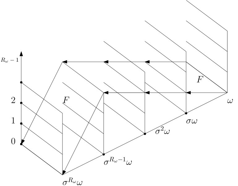 Figure 1
Peer Reviews
No public reviews on file for this paper yet. If you reviewed it on a platform where reviews are public (OpenReview, ICLR, NeurIPS, ICML), you can paste yours below so the community can read it here.
Videos
No videos yet. Explain this paper in a talk, walkthrough, or lecture? Add one.
\setremarkmarkup
(#2)
Quenched decay of correlations for slowly mixing systems
Wael Bahsoun*†*
Department of Mathematical Sciences, Loughborough University, Loughborough, Leicestershire, LE11 3TU, UK
,
Christopher Bose*∗*
Department of Mathematics and Statistics, University of Victoria, PO BOX 3045 STN CSC, Victoria, B.C., V8W 3R4, Canada
and
Marks Ruziboev*‡*
Abstract.
We study random towers that are suitable to analyse the statistics of slowly mixing random systems. We obtain upper bounds on the rate of quenched correlation decay in a general setting. We apply our results to the random family of Liverani-Saussol-Vaienti maps with parameters in chosen independently with respect to a distribution on and show that the quenched decay of correlation is governed by the fastest mixing map in the family. In particular, we prove that for every , for almost every , the upper bound holds on the rate of decay of correlation for Hölder observables on the fibre over . For three different distributions on (discrete, uniform, quadratic), we also derive sharp asymptotics on the measure of return-time intervals for the quenched dynamics, ranging from to to respectively.
Key words and phrases:
Random dynamical systems, slowly mixing systems, quenched decay of correlations.
1991 Mathematics Subject Classification:
Primary 37A05, 37E05
WB and MR would like to thank The Leverhulme Trust for supporting their research through the research grant RPG-2015-346. CB’s research is supported by a research grant from the National Sciences and Engineering Research Council of Canada. The authors would like to thank V. Baladi for useful communications and helpful comments.
Contents
-
5.1 Sharp asymptotics on the measure of return-time intervals
-
5.2 Natural probability distributions on the parameter space
-
6 Proof of existence of absolutely continuous mixing sample measures
-
8.1 Decay of future correlations (Proof of Theorem 4.2 item (i))
1. Introduction
In this paper we study statistical properties of systems that evolve according to deterministic laws driven by a random process. Such systems are called random dynamical systems and they are often studied via analysis of a related deterministic system, the skew product map given by:
[TABLE]
where is a family of transformations that map , the phase space, into itself, and is a measure preserving map on , the noise space. The ’s are often referred to as the fibre maps and is called the base map or the driving system. The fibre maps are the deterministic components of the random system, while the base map invokes the required randomness, or time dependence, or parameter drift in the system.
Recently there has been a remarkable interest in studying statistical limit theorems for random dynamical systems [1, 4, 5, 9, 10, 12, 13, 15, 21]. Most of these results assume some knowledge about the rate of correlation decay of the random system under consideration. In this work, we develop random towers that are suitable to study quenched111Quenched results in random dynamical systems refer to pathwise results for almost every . correlation decay for slowly mixing random systems. We obtain a general result on the rate of quenched correlation decay. Moreover, we apply our results to answer the following questions: in what way does an individual map , or a group of ’s, dictate the rate of quenched222In a simple model, yet important in the study of intermittent transition to turbulence [23], the first question was answered in [6] only for the annealed dynamics; i.e., for the dynamics averaged over , and only for a specific distribution on . Precisely [6] considered a system that has only two fibre maps and with the base system being a Bernoulli shift. correlation decay of the random system? A second question is: how does the distribution on (the measure preserved by ) effect the quenched statistics of the system? We answer the above two questions in the framework of the Pomeau-Manneville family [23] using the version popularised by Liverani-Saussol-Vaienti [17]. Such systems have attracted the attention of both mathematicians and physicists (see [16] for a recent work in this area). In particular, for Liverani-Saussol-Vaienti (LSV) maps with parameters in and base dynamics we show via a general random tower construction, that the quenched decay of correlation is governed by the fastest mixing map. Precisely, we prove that is an upper bound on the rate of quenched decay of correlation, for all . To illustrate the role that plays in the quenched decay rate, and to address the second question above, we also obtain sharp asymptotics on the position of return time intervals for the quenched dynamics in the Liverani-Saussol-Vaienti family that depend on the randomising distribution. In particular, we show how different distributions on (discrete, uniform, quadratic) change the sharp asymptotics on the position of return time intervals for the quenched dynamics from to to .
In Section 2 we recall standard definitions and notation from random dynamical systems and present various natural notions of correlation decay in this setting. In Section 3 we build random towers for our system and detail the dynamical hypotheses that are in force throughout the paper. Our main general results are contained in Section 4 (Theorems 4.1 and 4.2) where we prove existence and correlation decay estimates respectively for the dynamics on the random towers. In Section 5 we present detailed computations applying our general results to the case of random LSV maps on the interval. Three different randomising distributions are investigated: discrete, uniform and quadratic. At the end of Section 5 we also compute exact asymptotics for the measure of the return sets on the base of the random towers. In Section 6 we prove Theorem 4.1. The expansion and distortion conditions and related estimates are the main tools used in this section. In the next section, Section 7, we introduce random stopping times and derive asymptotics on their distributions in preparation for a coupling argument. In Section 8 we obtain decay of correlation estimates (upper bounds) for observables on our random towers. Both future and past decay estimates are derived. We conclude with Section 9 where we present some technical results that are used repeatedly in the paper. Notation: We use if there exists universal constant such that ; , , will have their usual meaning.
2. Random dynamical systems
Let be a Borel probability space, let be equipped with product measure and let denote the preserving two-sided shift map. Let be a measurable space. Suppose that is a family of measurable maps defined for -almost every such that the skew product
[TABLE]
is measurable with respect to were denotes the -th coordinate of . In order to simplify notation, we will normally write when there is no danger of confusion. So, for example, . The resulting i.i.d. random map associated to the family can be viewed as follows: letting denote the fiber over and we have . We say that is a -invariant measure if for any . Assume that forms measurable partition333This is satisfied, for example, when is Hausdorff so that is closed. of . We are interested in -invariant probability measures, , such that , where is the projection onto . Then by Rokhlin’s disintegration theorem (see [22] or [24] ), for any such measure there exists an (essentially unique) system of probability measures on such that for any
[TABLE]
It is easy to check that is -invariant if and only if for - a.e. , a property we naturally refer to as equivariance (or simply equivarariance, when the random map is understood) of the family .
In this paper we study statistical properties of the equivariant family of measures for -almost every , when is absolutely continuous with respect to Lebesgue measure on . More precisely we study future and past quenched correlations: given define future and past fibre-wise correlations
[TABLE]
Definition 1**.**
Let and be two Banach spaces on and let be a sequence of positive numbers such that . We say that admits quenched decay of correlations at rate if for -almost all and for any and there are constants and such that
[TABLE]
Remark 1*.*
Note that if is -integrable, then this implies the same rate for the integrated correlations; i.e., . The importance of knowing the rate of the integrated correlations is due to its relation to the annealed correlations of the skew product. Indeed, setting and we have
[TABLE]
3. Abstract tower setting
A main tool, in particular in the absence of spectral techniques, to study statistical properties of dynamical systems is the so called Young Tower [26, 27]. Young Towers have been used extensively to obtain rates of decay of correlations for nonuniformly hyperbolic systems (see for example [2, 3, 11, 19] and references therein). In this section we describe random towers which were first considered in [7] to study quenched statistical properties of i.i.d. unimodal maps. Later the work of [7] was extended in [8] to cover a wider class of i.i.d. unimodal maps. Building on ideas from [7, 8] we study random towers with slowly decaying tails. Let be a measurable set with . Consider a family of maps , where depends only on zeroth coordinate of . We say that admits a random tower on if for almost every there exists a countable partition of and a return time function that is constant on each such that for -almost every and -almost every Given the above information we define a random tower for almost every as
[TABLE]
and random tower map by
[TABLE]
Denote by the th level of the tower, which is a copy of ; for instance and . Let . Then is a fibered system on ; see Figure 1 for a pictorial representation.
Notice that induces a countable partition on each :
[TABLE]
For , let denote the first return time to the base of the tower i.e.
[TABLE]
The reference measure and -algebra on naturally lifts to and by abuse of notation we call it . The lifted -algebra will be denoted by . Next we define the separation time for almost every by setting if and lie in different towers and if then
[TABLE]
Below we refer to as the zeroth level of the tower. We assume that the random tower satisfies the following properties.
- (P1)
Markov: for each the map is a bijection;
- (P2)
Bounded distortion: There are constants and such that for all and each the map and its inverse are non-singular with respect to with corresponding Jacobian which is positive and for each satisfies the following
[TABLE]
- (P3)
Weak expansion: is a generating partition for i.e. diameters of the partitions converge to zero as tends to infinity;
- (P4)
Return time asymptotics: There are constants , , , , , a full measure subset and a random variable such that
[TABLE]
- (P5)
Aperiodicity: There are and such that g.c.d. and so that for almost every and we have .
- (P6)
Finiteness There exists an such that for all .
- (P7)
Annealed return time asymptotics: There are constants , and such that .
3.1. Tower projections
For almost every and we define tower projections as . Then is a semi-conjugacy i.e. . Indeed, for we have . On the other hand, since
[TABLE]
Now, if is an absolutely continuous family of -equivariant probability measures on , then is a family of - equivariant probability measures on . Since each is nonsingular, if is such that then , which implies , consequently . Therefore each is absolutely continuous.
4. Statement of main results
In this section we state general theorems concerning quenched correlation decay for slowly mixing systems. We start this section by introducing some function spaces on , which are necessary to state the theorems. These spaces appeared in the present form in [7]. Below we let constants , , , be as in (P2) and (P4) above and set
[TABLE]
Let be a random variable with and
[TABLE]
Define the space of random bounded functions as
[TABLE]
and a space of random Lipschitz functions
[TABLE]
Finally we let be a -algebra on defined as follows: if and only if for each the intersection . Let be a fibered equivariant family of measure i.e. . Let and . Then is -invariant (for the skew product on ). We say that is exact/mixing for if is exact/mixing for the skew product . We can formulate equivalent conditions as follows.
Definition 2**.**
- (i)
The fibered system is exact iff is trivial; i.e., for any , either for almost all , or for almost all , .
- (ii)
The random skew product is mixing iff for all ,
[TABLE]
We note that in our situation exactness implies mixing ([7], section 4). The first result is the existence of absolutely continuous sample measures.
Theorem 4.1**.**
Let be the fibered system described above. There exists an -equivariant family of absolutely continuous sample probability measure defined for almost every , which is exact, and hence mixing. Moreover, there exists satisfying (4.1) such that for almost every .
The next main result is about the decay of future and past quenched correlations.
Theorem 4.2**.**
Let . Let be the function given in Theorem 4.1. There exits a full measure set and a random variable on such that for every there exits a constant such that for every
- (i)
“Future” operational correlations :
[TABLE]
- (ii)
“Past” operational correlations :
[TABLE]
Moreover, there exist constants , , such that
[TABLE]
Remark 2*.*
A quenched correlation decay rate of the form , which is analogous to what one expects in the deterministic setting, cannot be achieved since we want to get information on the integrability of the in Theorem 4.2. The shift of the Lipschitz constant , and hence the dependence of that constant on , in equation (8.7) and the non-uniformity of the tail in (P4) are the main reasons for getting a rate at the order , for any . See Footnote 7 for more details.
5. Applications to random LSV maps
In this section we illustrate our results with applications to the family of intermittent LSV maps as described in [17]. Let and consider defined as
[TABLE]
To define a random LSV map we fix two positive numbers and let be a probability measure on . Set and . Then the shift map preserves . Let be the projection to the zeroth coordinate and let . We consider the skew product defined by
[TABLE]
Compositions of are given by .
For each we define a sequence of pre-images of as follows. Let , and
[TABLE]
Further let
[TABLE]
The sequences and will allow us to define the random tower structure. First of all notice that from the definition of we have , . Let . The sequence generates a partition on each . Define the return time by setting
[TABLE]
A fibered system is obtained by defining a tower over each by
[TABLE]
The fibered map from equation (3.1) can be expressed in this notation as follows: Let over , with . There are two cases. If , then since . On the other hand, if then , where , so the interval is mapped bijectively to by . Therefore in this case we have .
Proposition 5.1**.**
The fibered system with fibered map defined above satisfies properties (P1)-(P3) and (P5). In particular, the distortion condition (P3) is satisfied for any and .
Proof.
Since every map in the family expands by at least a factor of on return to the base interval , with full returns, we see that the Markov and weak expansion properties are satisfied. Furthermore, for each , , which implies that the aperiodicity condition (P5) is satisfied. Since every has negative Schwarzian derivative and this property is preserved under composition, we obtain the bounded distortion condition (P3) using the Koebe principle. See Lemmas 4.8 and 4.10 in [6] for computations related to Schwarzian derivatives and [20] for more details about the use of the Koebe principle. This completes the proof. ∎
It remains to establish appropriate estimates on the return time asymptotics as in (P4) and (P7) and the uniform bound in (P6). Observe, in view of the return-time formula (5.4), that
[TABLE]
We will estimate terms on the right hand side of this expression. Let (respectively ) denote the special sequences of all (respectively, all ). Following Lemma 4.4 in [6], we obtain coarse estimates on the location of the . Translated into our setting these estimates imply, for every ,
[TABLE]
It is well known (see [27] section 6, for example) that so if we define and write then . We define and analogously using . Since, this implies for some independent of . This proves (P6).
We now check that assumption (P4) is satisfied. Using definition (5.1) and the estimate , valid for , and by substituting we obtain
[TABLE]
Iterating this one-step estimate along the sequence , we obtain
[TABLE]
Combining equations (5.8) and (5.6) implies that, for any parameter
[TABLE]
where we have introduced notation for the sequence of independent random variables and for
[TABLE]
From now on we write . Note that for every .
**Assumption (A1) (Asymptotics on expectations)
**Assume444Below in the examples, we will show that the assumption is satisfied for different types of distributions. In particular, we will show how different measures lead to different tail asymptotics. there are constants and a constant such that the following holds:
[TABLE]
Fix any . Pick so that for all ,
[TABLE]
Note that, given expression (5.11), depends only on the choice of , and in particular is independent of . Set .
Lemma 5.2**.**
For each we have
[TABLE]
Proof.
We may apply the classical result of Hoeffding (see [14] Theorem 1, or [18] Lemma 1.2) to the sequence of independent random variables , noting that instead of the bound we have , accounting for the extra factor in the exponential. ∎
Next, we apply the previous lemma to obtain a large deviation estimate on the normalized sums of . For each :
[TABLE]
where in the last line we have used equation (5.12). Now define
[TABLE]
If then equation (5.9) implies that
[TABLE]
and hence
[TABLE]
provided . We may take and and in (P4). Note that the constant is independent of and . Finally, we estimate, for and fixed
[TABLE]
for suitable constants and . We can remove the restriction by substitution of a larger constant in the final expression
[TABLE]
completing the second condition in (P4). Finally we verify (P7).
First, we have
[TABLE]
where we have used the fact that is -invariant to write . Now recall that and . Using this fact, (5.17), (5.15) and , we obtain
[TABLE]
Choosing and completes the verification of (P7).
Theorem 5.1**.**
Let be fixed and equipped with product probability measure and left shift . Let be a random family of LSV maps with respect to the measure . Assume condition (A1) holds for the asymptotic expectations. Then there exists a family of absolutely continuous sample stationary measures on , for almost every (i.e. ). The system is mixing, i.e., setting , for all ,
[TABLE]
Moreover, for every there exists a full measure subset such that for every there exists so that for any , , the class of Hölder functions on , we have
- (i)
“Future” correlations :
[TABLE]
- (ii)
“Past” correlations :
[TABLE]
Finally, there exist constants , and such that the random variable satisifies the following tail estimates: for all
[TABLE]
In particular, is integrable. Every can be used by choosing555Recall that is the regularity parameter in the distortion condition (P2). so that .
Proof.
Proposition 5.1 establishes conditions (P1) - (P3) and (P5). Since we are assuming (A1), condition (P4) follows from equations (5.5) and (5.15) with constants . The second condition in (P4) holds because of equation (5.16). (P7) is verified in (5.18).
Theorem 4.1 therefore applies and gives existence and mixing of the sample stationary measures . Finally we apply Theorem 4.2 to obtain the decay of correlations.
For and define . Then we have . Now, to apply Theorem 4.2 it is sufficient to show and . The latter is obvious, since the projection is nonsingular and hence, for a.e. we have . For the former one we first note that since we have . Hence, for any we have the inequality
[TABLE]
Now since the inequality (5.19) implies
[TABLE]
∎
5.1. Sharp asymptotics on the measure of return-time intervals
Although we will not need lower bound estimates on the to prove the main results in this paper, it is not difficult to identify conditions (see Assumption (A2) below) under which the upperbounds from the previous section are sharp. This condition will hold for all of the examples discussed in this paper.
Notice that from equation (5.15) and the summability derived in equation (5.16), an application of Borel-Cantelli yields, for almost every ,
[TABLE]
Keeping in mind that was arbitrary (and working through a sequence of choices increasing to , applying Borel-Cantelli at each step) we obtain a set of full measure such that for every we have
[TABLE]
Now we concentrate on deriving lower bounds. Using definition (5.1) and the estimate , valid for , and by substituting we obtain
[TABLE]
Iterating (5.21) we obtain
[TABLE]
Clearly and the same is true of since
[TABLE]
In order to estimate note that from equation (5.20), for all sufficiently large (depending on ), for ,
[TABLE]
From now on we write . In addition to Assumption (A1) we now assume666We will see that for many examples, including the ones presented in the next section, Assumption (A2) will hold. the following asymptotics on the :
Assumption (A2) (Asymptotics on expectations revisited)
[TABLE]
Another large deviations estimate as in the preceding section will give, for each an integer so that for all , and
[TABLE]
Once again, application of Borel-Cantelli implies there exists a random variable , finite almost everywhere, such that for all
[TABLE]
and for each there are constants and so that
[TABLE]
The factor in equation (5.24) is necessary to account for the two terms and in equation (5.22). Returning to equation (5.24), another sequence of Borel-Cantelli reductions over the parameter decreasing to gives a full measure set such that for every
[TABLE]
We have therefore established the following (fibre-wise, or quenched) exact asymptotics
Proposition 5.3**.**
For random LSV maps as described in Theorem 5.1, assuming asymptotic growth conditions (5.11) and (5.23), we have the following exact asymptotics: There is a full measure subset such that for all , for all we have
[TABLE]
5.2. Natural probability distributions on the parameter space
In this subsection we verify assumptions (A1) and (A2) for some natural probability distributions on .
5.2.1. Example: Discrete distribution.
Here we assume is a discrete probability distribution; for concreteness, with and .
Lemma 5.4**.**
Therefore, in condition (5.11) we can take and .
Proof.
Write where
[TABLE]
Using -invariance of , a direct calculation shows
[TABLE]
while
[TABLE]
Therefore,
[TABLE]
whereas
[TABLE]
for . It follows that
[TABLE]
where . Therefore Assumption (5.11) is satisfied by taking and . ∎
We now show the upperbound on the obtained above is sharp.
Proposition 5.5** (Sharp asymptotics for the discrete probability distribution).**
For almost every
[TABLE]
where .
Proof.
We only need to verify Assumption (A2) and apply Proposition 5.3.
[TABLE]
Since we have verified Assumption (A2). ∎
5.2.2. Example: Uniform distribution.
Here we assume is the uniform probability distribution on , that is, for ,
[TABLE]
We start with a lemma that will allow us to compute the appropriate expectations in condition (5.11).
Lemma 5.6**.**
Let . Then, as
[TABLE]
Proof.
We have
[TABLE]
∎
As in the previous section, we decompose according to equation (5.26).
Using invariance of and Lemma 5.6 with and , respectively, we obtain
[TABLE]
It follows that . Now apply Lemma 9.2 of the Appendix to compute the asymptotics for the sum:
[TABLE]
Therefore we can take and in Assumption (A1)
Proposition 5.7** (Sharp asymptotics for the uniform probability distribution).**
For almost every
[TABLE]
where .
Proof.
We verify Assumption (A2) and apply Proposition 5.3.
[TABLE]
We can evaluate the individual expectations using Lemma 5.6 to obtain:
[TABLE]
Now, two applications of Lemma 9.2 from the Appendix shows
[TABLE]
Applying this to the first estimate gives
[TABLE]
Since we have verified Assumption (A2). ∎
5.2.3. Example: Quadratic distribution.
Here we assume is the quadratic probability distribution on , given by
[TABLE]
Again, we begin with a simple lemma that will allow us to estimate the expectations.
Lemma 5.8**.**
Let . Then, as
[TABLE]
Proof.
We have
[TABLE]
∎
Writing as in equation (5.26), using invariance of and Lemma 5.8 with we obtain
[TABLE]
It follows that after which an application of Lemma 9.2 of the Appendix implies
[TABLE]
We take and in the assumption (5.11). For this example, lower bounds can also be obtained by essentially following the steps in the previous example and using Lemma 5.8 in place of Lemma 5.6.
Proposition 5.9** (Sharp asymptotics for the quadratic probability distribution).**
For almost every
[TABLE]
where .
Proof.
We verify Assumption (A2) and apply Proposition 5.3. The key estimates are
[TABLE]
and
[TABLE]
where we have again used Lemma 9.2 in the Appendix to estimate the sum and verify Assumption (A2) for this example. ∎
6. Proof of existence of absolutely continuous mixing sample measures
6.1. Measure of the tail of the tower
Lemma 6.1**.**
.
Proof.
The bounds on imply that . Hence
[TABLE]
∎
6.2. Distortion estimates
Here we prove consequences of bounded distortion which are key for many of the later computations. For any
[TABLE]
Lemma 6.2**.**
For any , and the following inequality holds
[TABLE]
where is as in (3.4).
Proof.
The collection is a partition of and for any each contains a single element of For let be the number of visits of its orbit to up to time . Since the images of before time will remain in an element of all the points in have the same itineraries, up to time and so is constant on Therefore for the projection of onto (i.e. if then ). Thus for any from (3.4) we obtain
[TABLE]
∎
Corollary 6.3**.**
For any , is a bijection and for each we have
[TABLE]
Proof.
Lemma 6.2 implies Integrating both sides of this inequality with respect to over gives
[TABLE]
which finishes the proof. ∎
Lemma 6.4**.**
- (i)
There exists a constant such that for all and ,
[TABLE]
- (ii)
Let be a family of absolutely continuous probability measures on with . For every let and . There exists such that for each , for all we have
[TABLE]
where is as in (3.4).
Proof.
To prove the item (i) we estimate the density at an arbitrary point and consider three different cases according to the position of . First of all, for any , from Corollary 6.3 we have
[TABLE]
Since choosing finishes the proof for the case
For with we have Since for any
[TABLE]
Finally, let for Then for any the equality holds. Hence, for all Therefore, by the chain rule we obtain Hence the problem is reduced to the first case since
[TABLE]
This finishes the proof of item (i).
To prove the item (ii) we first note that is invertible. So for any there is a unique such that and
[TABLE]
Let then for , using Lemma 6.2 and assumption on we obtain
[TABLE]
∎
Remark 3*.*
It is important to note that the constant does not depend on . Moreover, if and are such that the orbits see sufficiently many returns to the base, so that , then the upperbound in (ii) becomes . The elements for which this holds are independent of the starting measure .
6.3. Proof of Theorem 4.1
Proof of Existence.
Recall that . Recall the definitions of and in (6.1), and for let
[TABLE]
where . Clearly, is a density on such that for . Below we consider two cases depending on . First, notice that if then is a bijection. For , let be such that , and . By the choice of there exists such that . The bounded distortion condition implies that
[TABLE]
Notice that the constant in equation (6.4) is independent of , and Hence for all letting we have
[TABLE]
Integrating both sides of the latter inequality over with respect to implies
[TABLE]
On the other hand, if such that for then . Hence we can apply (6.5). Futher define
[TABLE]
As above for . For , we write as a convex combination of and obtain
[TABLE]
Hence, is a uniformly bounded family. Notice that if and then . Taking this into account for all such that we have
[TABLE]
where we have used equation (6.4) in the last step.
Hence (i.e. ). Since, defines separable metric space structure on for each , we can find a subsequence which is convergent pointwise. By diagonal argument we then construct convergent subsequence for every . The limiting measure is -equivariant i.e. . Moreover, and by construction.
Exactness of the system can now be verified using the same method as detailed in [7]. ∎
7. Random coupling
7.1. Estimates on the random recurrence times for the base
For a single map, the recurrence time of the base with the base gives a key construction parameter for coupling arguments. In the setting of random maps, this recurrence time is dependent. Our first task is to obtain a suitable version of the recurrence time (see below, and its use in the following Lemma 7.2). At this stage, it is useful for the reader to recall from section 3 our assumptions (P1)-P(7); in particular that in (P4). Moreover, recall the regularity class of the equivariant densities defined by the random variable from Theorem 4.1.
Lemma 7.1**.**
Let and be from the aperiodicity condition (P5). There is an so that for every there are nonnegative integers such that
[TABLE]
Proof.
See Lemma A2 [25]. ∎
For define a random variable by
[TABLE]
Recall that every base .
Lemma 7.2**.**
For each there is a constant so that for almost every ,
[TABLE]
Proof.
The result follows from the aperiodicity condition (P5) and bounded distortion (P2). First, suppose and , satisfying
[TABLE]
Then, since are bijections when restricted to , using bounded distortion, we get
[TABLE]
Now, for , Lemma 7.1 implies can be written as a composition of (with at most terms). Iterating the above estimate and using the lower bounds given in condition (P5) implies the existence of the required lower bound . ∎
Remark 4*.*
From the proof of the previous lemma, it is clear that one should not expect a lower bound on the , uniform over all .
7.2. Random stopping times
Let . Denote by the relative product over , that is . These are measurable subsets of the appropriate product spaces ( in the case of , for example), and naturally carry the measures and respectively. We can lift the tower map to a product action on with the property by applying in each of the coordinates.
With respect to this map, we define auxiliary stopping times to the base as follows:
Let be the constant given in Lemma 7.1. For set
[TABLE]
and so on, with the action alternating between and . Notice that for odd ’s the first (resp. for even ’s the second) coordinate of makes a return to .
Let be the smallest integer such that . Then we define the stopping time by
[TABLE]
Next define a sequence of partitions of so that is constant on the elements of for all . Given a partition of we write to denote the element of containing . With this convention, we let
[TABLE]
Letting be the projection to the first coordinate, we define
[TABLE]
Let be the projection onto the second coordinate. We define by refining the partition on the first coordinate, and so on. If is defined then we define by refining each element of in the first coordinate so that is constant on each element of . Similarly is defined by refining each element of in the second coordinate so that is constant on each new partition element. Now we define a partition of such that is constant on its element. For definiteness suppose that is even and choose such that . By construction such that and is spread around . We refine into countably many pieces and choose those parts which are mapped onto the corresponding base at time . Note that may not be measurable with respect to However, since and is defined by dividing into pieces where is constant, is measurable with respect to
7.3. Tail of the simultaneous return times
In this section we estimate the tail of the simultaneous return time . We start this section with the lower bound on the measure of the set that made return at time .
Lemma 7.3**.**
Let and be two probability measures on with densities . Let . For each , for each and such that we have
[TABLE]
where . We can fix , independent of , for all sufficiently large, i.e. .
Proof.
For definiteness assume is even. Then has the property and . Together with the definition of this implies . Therefore, letting we have
[TABLE]
Finally, item (ii) of Lemma 6.4 applied to implies that
[TABLE]
Now, the lemma holds with . In view of Remark 3 we can use for all sufficiently large. ∎
The next lemma estimates the distribution of ’s on by the measure of the tail of the random tower.
Lemma 7.4**.**
Let be as in Lemma 7.3. For each , for each and
[TABLE]
Proof.
Suppose that is even. Since is constant on the elements of for every we have
[TABLE]
Letting , we have
[TABLE]
Applying item (ii) of Lemma 6.4 we obtain
[TABLE]
Finally, since the density of is bounded above by the first item of Lemma 6.4 we have
[TABLE]
For odd the calculation is analogous and we obtain for all
[TABLE]
∎
Suppose we are given a sequence of positive integers with for all , denoted , and a positive integer . Define associated subsets of
[TABLE]
This is a partition into sets where a specified sequence of hitting times up to is attained:
[TABLE]
For fixed denote the cross section of at . Let . The following lemma gives a useful estimate on the size of the elements .
Lemma 7.5**.**
There exists a such that for each fixed ,
[TABLE]
where
[TABLE]
Proof.
Assume first that is even and let be as above. Let , . We first show that
[TABLE]
Indeed, for any with we have
[TABLE]
Hence we have
[TABLE]
Therefore,
[TABLE]
By induction, for any , we have
[TABLE]
A similar argument applies to obtain the same formula when is odd. Now by (i) of Lemma 6.4, we get
[TABLE]
Notice that, depends only on while depends only on . By definition of , we have . Therefore, the product on the right hand side of (7.1) is formed of independent random variables. Moreover, observe that depends only on and . Thus,
[TABLE]
Taking gives the desired estimate. ∎
We now present two lemmas that will be invoked in the proof of Proposition 7.8 below.
Lemma 7.6**.**
We have . Moreover, as .
Proof.
Using assumption (P7) and Lemma 9.1 in the appendix, we have
[TABLE]
Moreover; as . ∎
Lemma 7.7**.**
We have .
Proof.
Recall that ; i.e., does not depend on . Therefore,
[TABLE]
where we have used the first item of Lemma 6.4 and (P7). ∎
We can now present the main result of this section.
Proposition 7.8**.**
Let be given. Let and be two two families of probability measures on with densities . Let . Then there exists a constant and a subset of full measure and a random variable on such that for any the following holds
[TABLE]
Moreover, there exist , such that for any
[TABLE]
Proof.
Let . For a.e. we have777 Notice that we have chosen to keep the proof and the estimates of , and as simple as possible. One may try for sufficiently large so that decays faster than and remains integrable and to get a quenched decay rate of the form , for some , in Theorem 4.2. However, no matter how we choose , with as , a quenched correlation decay rate of the form , which is analogous to what one expects in the deterministic setting, cannot be achieved since we want to get information on the integrability of the in Theorem 4.2. The shift of the Lipschitz constant , and hence the dependence of that constant on , in equation (8.7) and the non-uniformity of the tail in (P4) are the main reasons for getting a rate at the order , for any .
[TABLE]
We will show that the term decays at the indicated log-polynomial rate (in ) while the term decays as stretched exponential, which implies the result. First, for the term we have:
[TABLE]
For each term in the sum (7.4), using Lemma 7.4 we obtain,
[TABLE]
For each , where is the full measure subset from condition (P4), we want to define a random variable such that for any we have for any , , so that we can apply the uniform decay rates from (P4). Below the constraint is crucial.
[TABLE]
We claim that has a stretched exponential tail.
[TABLE]
for an appropriate choice of , . Now, for using the fact that and Lemma 9.1 we can further upper bound the sum in the equation (7.5) by
[TABLE]
Now, inserting the estimate (7.6) back into equation (7.5) and substituting that result into (7.4) we obtain the final estimate on :
[TABLE]
Now we tackle the term by decomposing into two pieces. First for parameters and , and integer define
[TABLE]
We are going to pick the parameters , and later, but the idea is that for points in the first return times have many (at least ) large (bigger than ) gaps. Our decomposition will be according to this for :
[TABLE]
In order to estimate the first term in this expression, fix a sequence of integers for and define
[TABLE]
Then and by Lemma 7.5 we can estimate measures of the terms on the right by
[TABLE]
Now applying Lemmas 7.7 and 7.6 we obtain, assuming ,
[TABLE]
We pick large enough so that
[TABLE]
This shows . Since we want estimates over individual fibres we finally observe the above estimate shows except on a set of of measure at most . Once again, an application of Borel-Cantelli shows there is a full measure set and with stretched exponential tails (there exists and so that and such that, for every and , .
We now turn our attention to the complement of . Note that for each either or . Let us call those in the former class . The others we will call . Therefore, for fixed
[TABLE]
We move now to estimate the individual terms in the sum over terms. Note that each is measurable. Therefore we can write
[TABLE]
as a disjoint union. Recall that is measurable with respect to . Therefore, for each in the above decomposition, either or . Call the former and the latter . Finally, note that if is then . Now we estimate:
[TABLE]
Now, since each good in the above sum is a subset of that is we know that . Therefore, in the above product, considering only those factors in the product, and keeping in mind the lower bound given by Lemma 7.2 we get
[TABLE]
Finally, summing first over all the good and then over all for we obtain
[TABLE]
Set and obtain
[TABLE]
for all , giving the claimed stretched exponential decay. This completes the proof of the lemma. ∎
7.4. Coupling
Here we consider which is a mapping from into . Let be the partition of on which is constant. Let be stopping times on defined as
[TABLE]
For we define a separation time associated with as the smallest such that and lie in distinct elements of 888Notice that, for any if then and ..
Let and be two probability measures on with densities . Let and , then . The next lemma establishes the regularity of and .
Lemma 7.9**.**
- (1)
For any , with
[TABLE]
where is a constant. 2. (2)
For any ,
[TABLE]
where .
Proof.
Let , . For choose so that . Then
[TABLE]
where we have used . Similarly for the second item we have
[TABLE]
∎
Let be the partition of on which are constant. For let be the element containing . Given let be such that . For let For , let
[TABLE]
where is a small number that will be defined below. Since is constant on every , we have
[TABLE]
Note that, is the density of the part of which has not been matched up to time .
Lemma 7.10**.**
For all sufficiently small in (7.11), there exists independent of such that for almost every and for all
[TABLE]
We will introduce the following densities in order to prove Lemma 7.10. For let
[TABLE]
and for , let
[TABLE]
Lemma 7.10 then follows from the following lemma:
Lemma 7.11**.**
There exists such that for all sufficiently small the following holds: for any with and
[TABLE]
Proof.
By definition of and item (1) Lemma 7.9 of we have
[TABLE]
Since is constant on we let . We have
[TABLE]
Notice that in the latter inequality increases as increases. Allowing to depend on , and ,999Notice that when we can choose uniform for all and , allowing dependence only on and . for a given we can choose small enough so that
[TABLE]
we obtain
[TABLE]
By (7.12) and (7.14) we obtain
[TABLE]
Moreover, for we have
[TABLE]
Note that in the last inequality we have used . Finally, using the relation we have
[TABLE]
where .
Now, we show by an inductive argument that in (7.13) can be chosen independent of , , , . First of all notice that we can choose independent of for because
[TABLE]
Let and suppose that is small enough so that (7.16) holds for all and . Then by (7.12) we have
[TABLE]
which implies that . Therefore in (7.13) is bounded by . Hence by choosing we conclude that the estimate in (7.15) holds for . ∎
Lemma 7.12**.**
Let be as in Lemma 7.10. For almost every and all
[TABLE]
where .
Proof.
In Lemma 7.10 the estimates for the mass of after the iterate matching was given. Now we will relate that estimate to the iterates of . Define , as follows: for let
[TABLE]
where is as in (7.11). We first prove that . Below we use the notation to denote a measure whose density with respect to is . First of all recall that and write . We have
[TABLE]
Since, for any we have
[TABLE]
the first term in the final sum in (7.17) is bounded by . Now, we claim that all other terms in (7.17) vanish. Let be such that . By construction is a union of elements of and for (because for ). For by definition of the ’s we have . On the other hand, on . Hence for each and for every we have
[TABLE]
which finishes the proof of claim.
It remains to estimate . We have
[TABLE]
Note that on . Hence we have
[TABLE]
Let be such that . By Lemma 7.10 we have . Hence
[TABLE]
∎
8. Decay of correlation
The main result of this section is the following proposition.
Proposition 8.1**.**
For every there is a full measure set and a random variable such that for all probability measures on with , there is so that for any , we have
[TABLE]
Moreover, there exist , such that
[TABLE]
for some and .
Before proving the proposition, we prove the following auxiliary lemma.
Lemma 8.2**.**
There exists such that for all and for any
[TABLE]
Proof.
By definition we have
[TABLE]
Therefore, it remains to bound the density . Let . Any have unique pre-images . By definition we have
[TABLE]
Since is independent of this implies . ∎
Proof of Proposition 8.1.
Note that, by taking Lemma 7.12 implies
[TABLE]
By choosing so that , for any we have
[TABLE]
Now we estimate for . Let . We proceed as in equation (7.4) in the estimate of . For every we write
[TABLE]
Recall that there is a full measure set and a random variable which is finite on , and . Now define
[TABLE]
We now show that has a stretched exponential tail. Indeed,
[TABLE]
for an appropriate choice of , . Since , for any we have
[TABLE]
Therefore, by Proposition 7.8 and the definition of , for any we can estimate (8.3) as follows:
[TABLE]
Finally, using (8.4)
[TABLE]
Thus, combining (8.2) and (8.5) finishes the proof. ∎
8.1. Decay of future correlations (Proof of Theorem 4.2 item (i))
Let and . Also, let , and be the constants given in the definitions of and respectively. Let , where . Then , and for all . The second assertion is obvious by the choice of . For the third one we use the inequality . For the first claim we have
[TABLE]
For the correlations we have the following relation
[TABLE]
Let be a probability with density . Then by Proposition 8.1 for every we have
[TABLE]
Similarly, for the probability measure with the constant density we have
[TABLE]
Define . Substituting (8.7) and (8.8) into (8.6), and using the inequality we have
[TABLE]
Let . Then
[TABLE]
Now, if then
[TABLE]
If then we let
[TABLE]
Hence, for all we have obtained
[TABLE]
It remains to show has the desired decay rate. We write
[TABLE]
Notice that by the definition of we have
[TABLE]
Hence, we have
[TABLE]
Then the conclusion of the theorem holds with and .
8.2. Decay of past correlations
To obtain decay of past correlations we need to prove the results of Sections 7 and 8.1 with the corresponding shift on . Below we use the notation for .
Lemma 8.3**.**
Let and be two probability measures on with densities . Let . For each let . Then for any and where such that we have
[TABLE]
where . Dependence of on on can be removed if we only consider .
Lemma 8.4**.**
Let be as in Lemma 7.3. For each , let . For every and
[TABLE]
Proposition 8.5**.**
Let be given. Let and be two probability measures on with densities . Then there exists a constant and a subset full measure and a random variable which is finite on such that for any letting we have
[TABLE]
Moreover, there exist such that for any
[TABLE]
Proposition 8.6**.**
For every there is a full measure set and a random variable , which is finite on such that for all probability measures on with , there is so that for any letting we have
[TABLE]
Moreover, there exist , and such that
[TABLE]
Using the above statements and following the same strategy as in the proof of future correlations we conclude decay of past correlations.
9. Appendix
9.1. Sub-polynomial tail estimates
Lemma 9.1**.**
Let and . Then
[TABLE]
Proof.
The proof is based on integration by parts. Since is monotonically decreasing on for big enough, we have
[TABLE]
Let . Then first making change of variables and the integrating by parts times we obtain
[TABLE]
where . Since we conclude that , This shows that the dominant term in (9.1) is . ∎
Lemma 9.2**.**
Suppose and . Then
Proof.
A straightforward estimate, using the fact that shows that and . We work with the latter sum. An elementary estimate shows
[TABLE]
Therefore . We now estimate the integral.
[TABLE]
using integration by parts. The first term above is the claimed rate, and the second term is clearly . We will show the same is true for the third, integral term. We first upper-bound as follows:
[TABLE]
Now simply estimate the right hand side by
[TABLE]
Since both terms are in we are done. ∎
The reference list from the paper itself. Each links out to its DOI / PubMed record.
- 1[1] R. Aimino, M. Nicol, S. Vaienti, Annealed and quenched limit theorems for random expending dynamical systems . Probability Theory and Related Fields 162 (2015), no. 1-2, 233–274.
- 2[2] J. F. Alves, S. Luzzatto, V. Pinheiro, Markov structures and decay of correlations for non-uniformly expanding maps . Ann. Inst. H. Poincaré Anal. Non Linéaire , 22 (2005), no. 6, 817–839.
- 3[3] J.F. Alves, V. Pinheiro, Slow rates of mixing for dynamical systems with hyperbolic structures . J. Stat. Phys. 131 (2008), no. 3, 505–534
- 4[4] A. Ayyer, C. Liverani, M. Stenlund, Quenched CLT for random toral automorphisms . Discrete Contin. Dyn. Syst. 24, no. 2 (2009), 331–348.
- 5[5] W. Bahsoun, C. Bose, Mixing rates and limit theorems for random intermittent maps . Nonlinearity. Vol. 29 (2016), no. 4, 1417–1433.
- 6[6] W. Bahsoun, C. Bose, Y. Duan, Decay of correlation for random intermittent maps . Nonlinearity. Vol. 27 (2014), no. 7, 1543–1554.
- 7[7] V. Baladi, M. Benedicks, V. Maume-Deschamps, Almost sure rates of mixing for i.i.d. unimodal maps , Ann. Sci. École Norm. Sup. Vol. 35 (2002), no. 1, 77 –126. V. Baladi, M. Benedicks, V. Maume-Deschamps, Ann. Sci. École Norm. Sup. Vol. 36 (2003), 319–322 (corrigendum). V. Baladi, M. Benedicks, V. Maume-Deschamps, Correcting the proof of Theorem 3.2 and Corollary 5.2 in Almost sure rates of mixing for i.i.d. unimodal maps . ar Xiv:1008.5165 (corrigenda).
- 8[8] Z. Du, On mixing rates for random perturbations . Ph D Thesis, National University of Singapore, 2015.