Search for direct top squark pair production in events with a Higgs or $Z$ boson, and missing transverse momentum in $\sqrt{s}=13$ TeV $pp$ collisions with the ATLAS detector
ATLAS Collaboration

TL;DR
This paper reports a search for top squark pair production in proton-proton collisions at 13 TeV using the ATLAS detector, focusing on events with Z or Higgs bosons and missing transverse momentum, but finds no evidence of supersymmetry.
Contribution
It presents the first ATLAS search targeting top squark pairs decaying via Z or Higgs bosons, extending exclusion limits up to about 800 GeV for their masses.
Findings
No excess observed over Standard Model predictions.
Excludes top squark masses up to about 800 GeV at 95% confidence level.
Extends previous supersymmetry exclusion regions.
Abstract
A search for direct top squark pair production resulting in events with either a same-flavour opposite-sign dilepton pair with invariant mass compatible with a boson or a pair of jets compatible with a Standard Model (SM) Higgs boson () is presented. Requirements on additional leptons, jets, jets identified as originating from -quarks, and missing transverse momentum are imposed to target the other decay products of the top squark pair. The analysis is performed using proton-proton collision data at TeV collected with the ATLAS detector at the LHC in 2015--2016, corresponding to an integrated luminosity of 36.1 fb. No excess is observed in the data with respect to the SM predictions. The results are interpreted in two sets of models. In the first set, direct production of pairs of lighter top squarks () with long decay chains involving or…
Click any figure to enlarge with its caption.
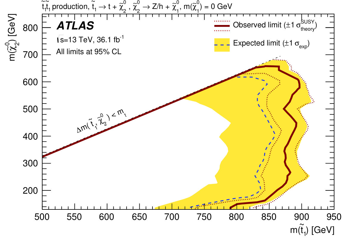 Figure 1
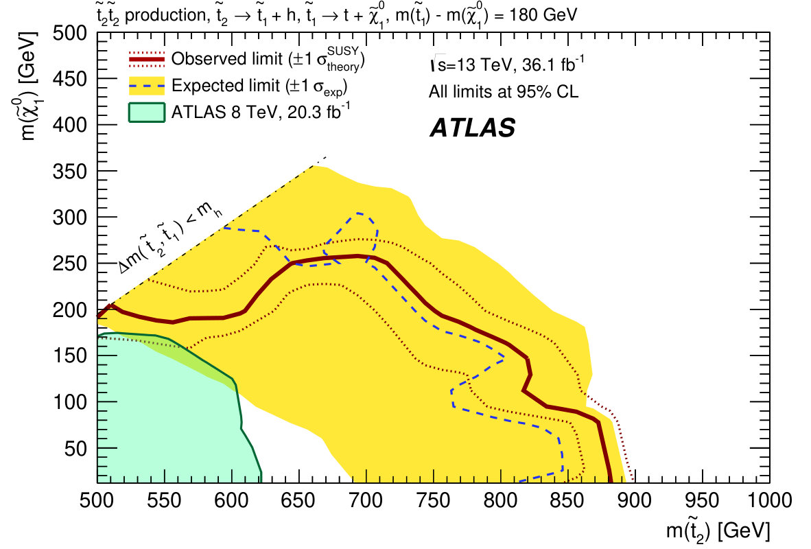 Figure 2
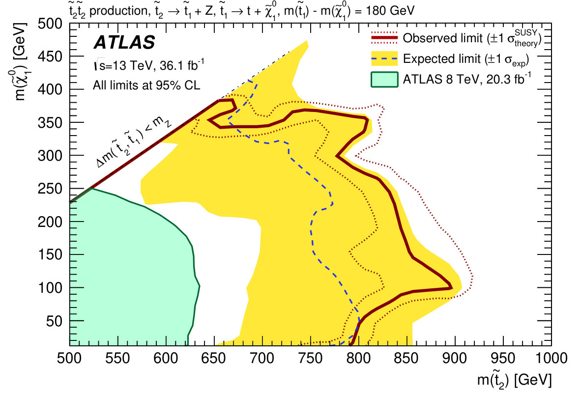 Figure 3
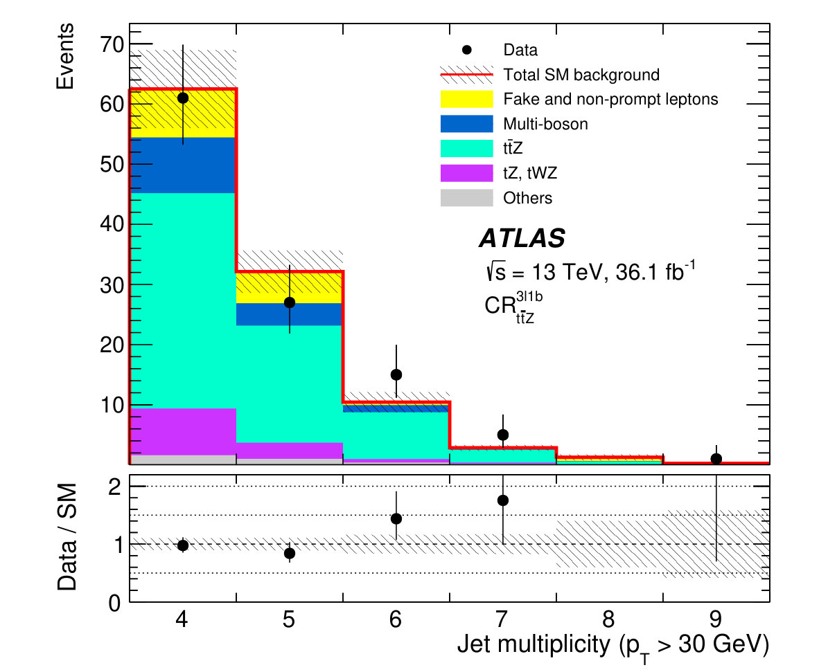 Figure 4
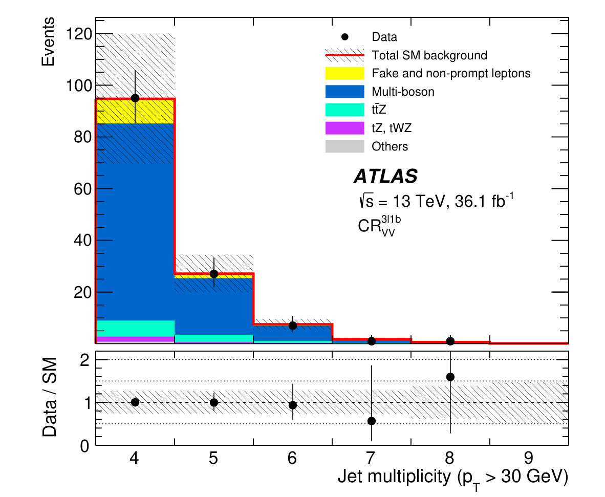 Figure 5
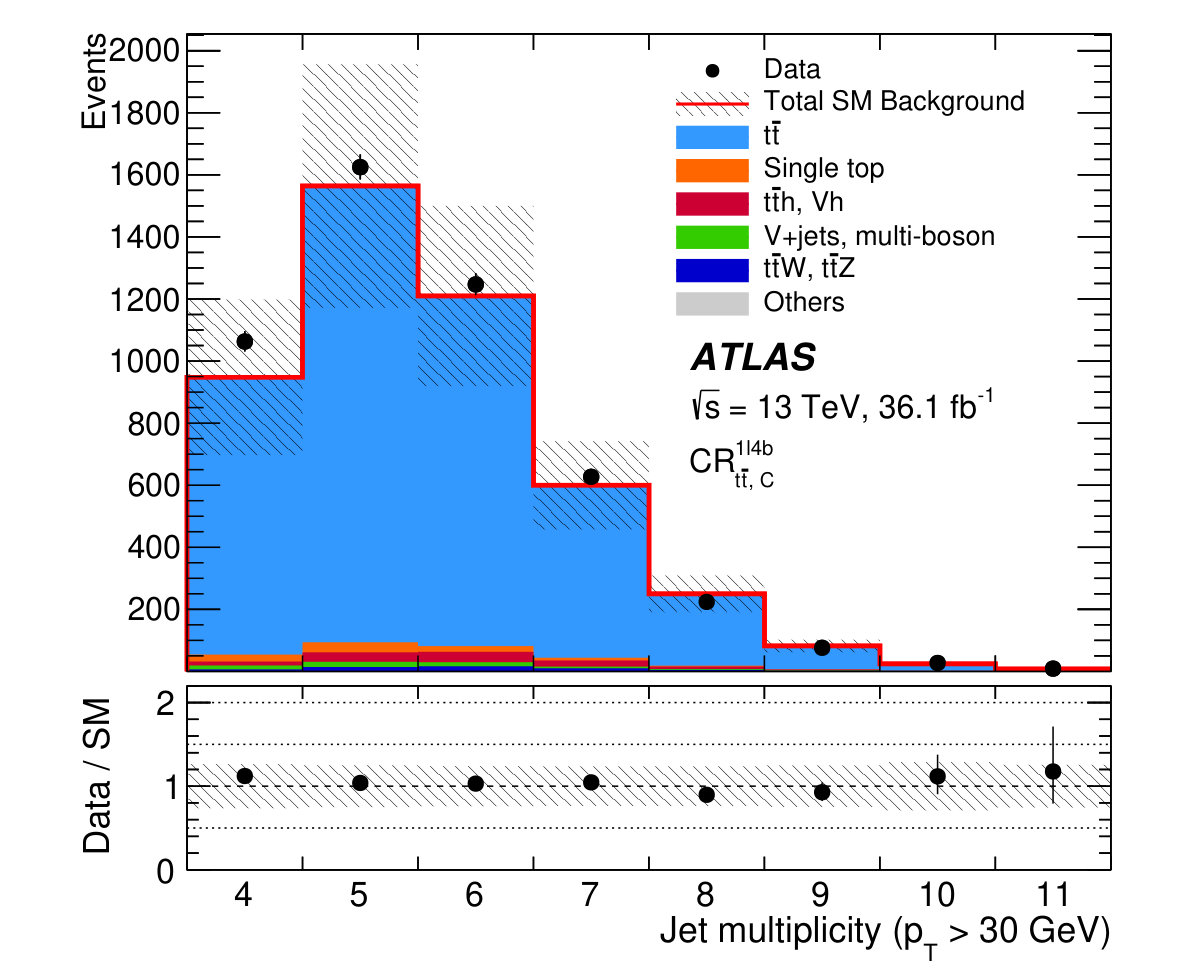 Figure 6
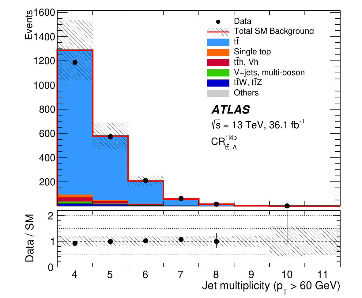 Figure 7
 Figure 8
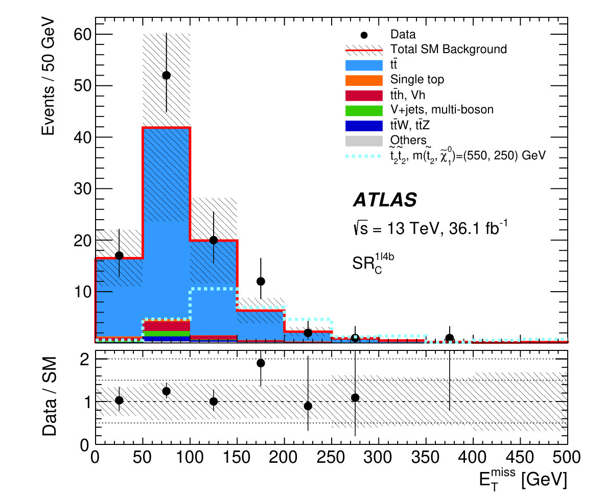 Figure 9
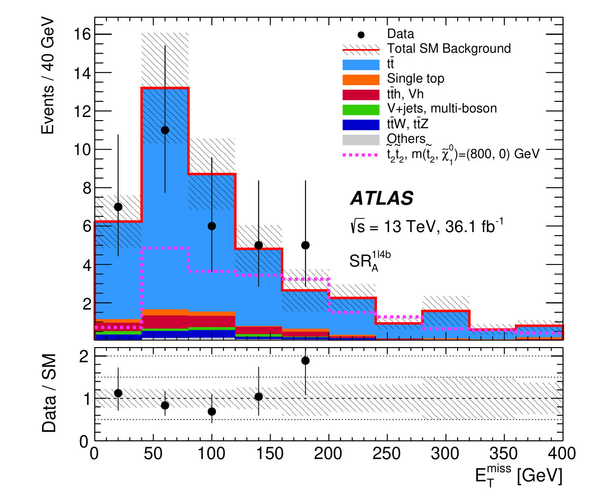 Figure 10
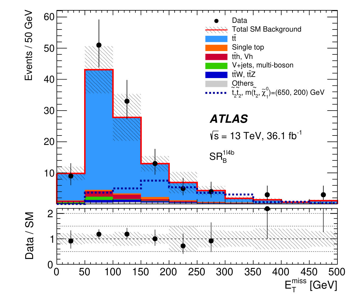 Figure 11
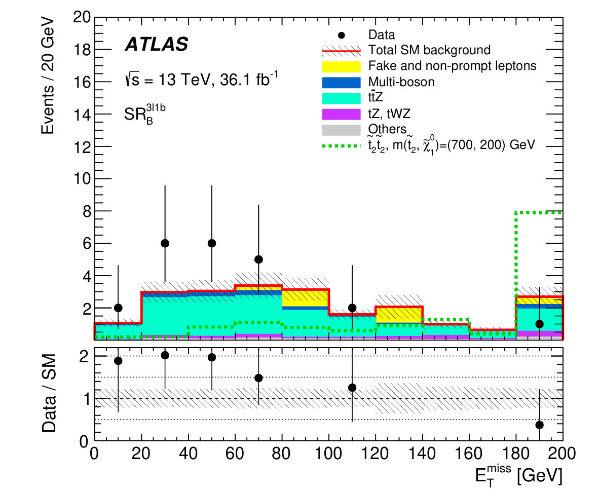 Figure 12
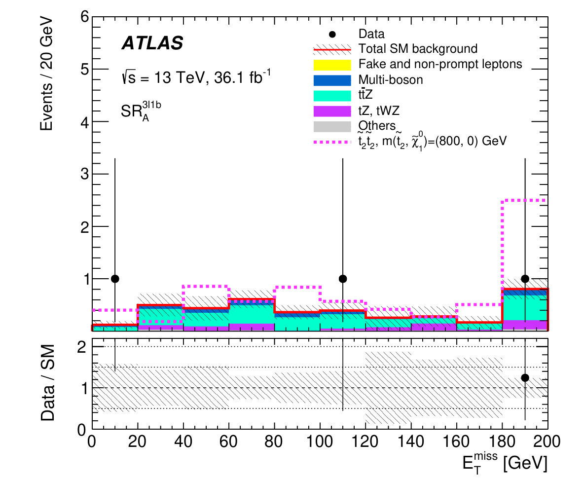 Figure 13
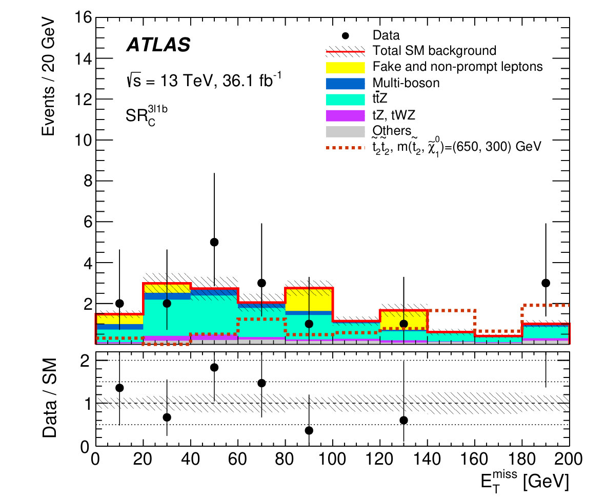 Figure 14
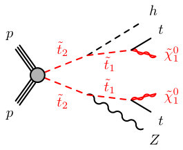 Figure 15
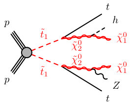 Figure 16
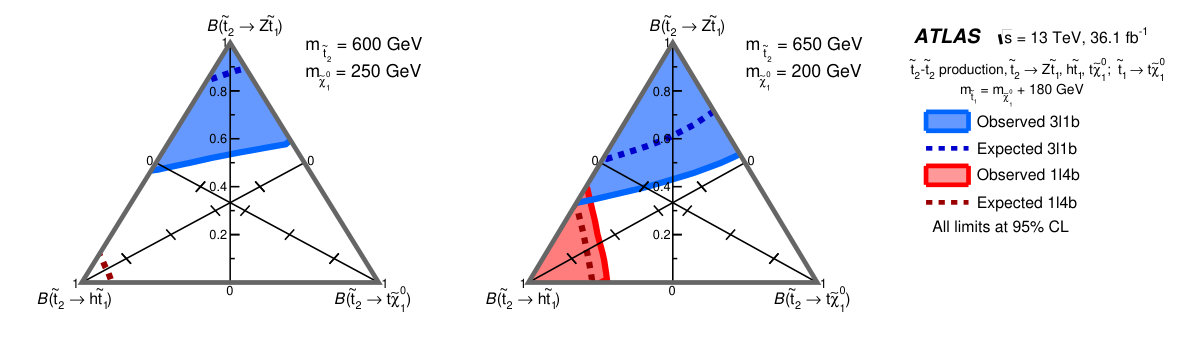 Figure 17
 Figure 18
 Figure 19
 Figure 20
| Physics process | Generator | Parton shower | Cross-section | PDF set | Tune |
| normalisation | |||||
| SUSY Signals | MadGraph5_aMC@NLO 2.2.3 [39] | Pythia 8.186 [40] | NLO+NLL [41, 42, 43, 44, 45] | NNPDF2.3LO [46] | A14 [47] |
| + jets | Sherpa 2.2.1 [48] | Sherpa 2.2.1 | NNLO [49] | NLO CT10 [46] | Sherpa default |
| + jets | Sherpa 2.2.1 | Sherpa 2.2.1 | NNLO [49] | NLO CT10 | Sherpa default |
| powheg-box v2 [50] | Pythia 6.428 [51] | NNLO+NNLL [52, 53, 54, 55, 56, 57] | NLO CT10 | Perugia2012 [58] | |
| Single-top | |||||
| (-channel) | powheg-box v1 | Pythia 6.428 | NNLO+NNLL [59] | NLO CT10f4 | Perugia2012 |
| Single-top | |||||
| (- and -channel) | powheg-box v2 | Pythia 6.428 | NNLO+NNLL [60, 61] | NLO CT10 | Perugia2012 |
| MadGraph5_aMC@NLO 2.2.2 | Pythia 8.186 | NLO [39] | NNPDF2.3LO | A14 | |
| Diboson | Sherpa 2.2.1 | Sherpa 2.2.1 | Generator NLO | CT10 | Sherpa default |
| MadGraph5_aMC@NLO 2.2.2 | Herwig 2.7.1 [62] | NLO [63] | CTEQ6L1 | A14 | |
| , | MadGraph5_aMC@NLO 2.2.2 | Pythia 8.186 | NLO [63] | NNPDF2.3LO | A14 |
| , | MadGraph5_aMC@NLO 2.2.2 | Pythia 8.186 | NLO [39] | NNPDF2.3LO | A14 |
| , , | MadGraph5_aMC@NLO 2.2.2 | Pythia 8.186 | LO | NNPDF2.3LO | A14 |
| Triboson | Sherpa 2.2.1 | Sherpa 2.2.1 | Generator LO, NLO | CT10 | Sherpa default |
| Requirement / Region | SR | SR | SR |
|---|---|---|---|
| Number of leptons | |||
| [GeV] | |||
| Leading lepton [GeV] | |||
| Leading jet [GeV] | |||
| Leading -tagged jet [GeV] | |||
| ( GeV) | |||
| [GeV] | |||
| [GeV] | – |
| Requirement / Region | SR | SR | SR |
| Number of leptons | 1–2 | 1–2 | 1–2 |
| [GeV] | – | 150 | 125 |
| [GeV] | – | – | |
| [GeV] | |||
| Leading -tagged jet [GeV] | – | – | 140 |
| [GeV] | 95–155 | – | – |
| [GeV] | – | – | |
| ( >60 GeV) | – | ||
| ( >30 GeV) | – | – |
| Requirement / Region | CR | CR |
| Number of leptons | ||
| [GeV] | ||
| Leading lepton [GeV] | ||
| Leading jet [GeV] | ||
| 0 | ||
| GeV) | ||
| [GeV] | – | |
| [GeV] | – | – |
| CR | CR | |
| Observed events | ||
| Total (post-fit) SM events | ||
| Fit output, multi-boson | ||
| Fit output, | ||
| Fake or non-prompt leptons | ||
| , | ||
| Others | ||
| Fit input, multi-boson | ||
| Fit input, |
| Requirement / Region | CR | VR | CR | VR | CR | VR |
| Number of leptons | 1–2 | 1–2 | 1–2 | 1–2 | 1–2 | 1–2 |
| [GeV] | – | – | 100 | 150 | 125 | 125 |
| [GeV] | 120 | 120 | 150 | 150 | ||
| Leading -tagged jet [GeV] | – | – | – | – | 140 | 140 |
| [GeV] | 95–155 | [95,155] | – | – | – | – |
| ( >60 GeV) | – | – | ||||
| ( >30 GeV) | – | – | – | – |
| CR | VR | CR | VR | CR | VR | |
| Observed events | ||||||
| Total (post-fit) SM events | ||||||
| Fit output, | ||||||
| Single top | ||||||
| +jets, multi-boson | ||||||
| , | ||||||
| , | ||||||
| Others | ||||||
| Fit input, |
| SR | SR | SR | SR | SR | SR | |
| Total systematic uncertainty (%) | 20 | 24 | 15 | 22 | 17 | 30 |
| Diboson theoretical uncertainties (%) | 6.7 | 5.5 | 2.2 | <1 | <1 | <1 |
| theoretical uncertainties (%) | 10 | 10 | 4.4 | <1 | <1 | <1 |
| theoretical uncertainties (%) | – | – | – | 17 | 14 | 22 |
| Other theoretical uncertainties (%) | 9.0 | 6.8 | 5.4 | 1.6 | 2.4 | 1.7 |
| MC statistical uncertainties (%) | 8.5 | 18 | 6 | 7.3 | 5.2 | 13 |
| Diboson fitted normalisation (%) | 4.6 | 3.5 | 3.8 | <1 | <1 | <1 |
| fitted normalisation (%) | 12 | 11 | 13 | <1 | <1 | <1 |
| fitted normalisation (%) | – | – | – | 3.4 | 5.1 | 3.3 |
| Fake or non-prompt leptons (%) | – | 6.5 | – | – | – | – |
| Pile-up (%) | 4.7 | 2.8 | 0.6 | <1 | 1.4 | <1 |
| Jet energy resolution (%) | 2.0 | 2.7 | 3.0 | 5.3 | <1 | 13 |
| Jet energy scale (%) | 1.0 | 2.7 | 3.5 | 3.2 | 5.3 | 6.1 |
| resolution (%) | 5.3 | 2.6 | 1.6 | 6.8 | 6.5 | 4.0 |
| -tagging (%) | 2.4 | 1.5 | 3.0 | 6.8 | 2.9 | 3.5 |
| SR | SR | SR | |
| Observed events | |||
| Total (post-fit) SM events | |||
| Fit output, multi-boson | |||
| Fit output, | |||
| , | |||
| Fake or non-prompt leptons | |||
| Others | |||
| Fit input, multi-boson | |||
| Fit input, | |||
| [fb] | 0.13 | 0.10 | 0.16 |
| 0.42 | 0.93 | 0.23 | |
| SR | SR | SR | |
| Observed events | |||
| Total (post-fit) SM events | |||
| Fit output, | |||
| Single top | |||
| +jets, multi-boson | |||
| , | |||
| , | |||
| Others | |||
| Fit input, | |||
| [fb] | 0.21 | 0.40 | 0.43 |
| 0.63 | 0.82 | 0.11 |
Peer Reviews
No public reviews on file for this paper yet. If you reviewed it on a platform where reviews are public (OpenReview, ICLR, NeurIPS, ICML), you can paste yours below so the community can read it here.
Videos
No videos yet. Explain this paper in a talk, walkthrough, or lecture? Add one.
\AtlasTitle
Search for direct top squark pair production in events with a Higgs or boson, and missing transverse momentum in TeV collisions with the ATLAS detector
\PreprintIdNumberCERN-EP-2017-106 \AtlasJournalJHEP \AtlasAbstractA search for direct top squark pair production resulting in events with either a same-flavour opposite-sign dilepton pair with invariant mass compatible with a boson or a pair of jets compatible with a Standard Model (SM) Higgs boson () is presented. Requirements on additional leptons, jets, jets identified as originating from -quarks, and missing transverse momentum are imposed to target the other decay products of the top squark pair. The analysis is performed using proton-proton collision data at TeV collected with the ATLAS detector at the LHC in 2015–2016, corresponding to an integrated luminosity of 36.1 fb*-1*. No excess is observed in the data with respect to the SM predictions. The results are interpreted in two sets of models. In the first set, direct production of pairs of lighter top squarks () with long decay chains involving or Higgs bosons is considered. The second set includes direct pair production of the heavier top squark pairs () decaying via or . The results exclude at 95% confidence level and masses up to about 800 GeV, extending the exclusion region of supersymmetric parameter space covered by previous LHC searches.
1 Introduction
Supersymmetry (SUSY) [1, 2, 3, 4, 5, 6] is one of the most studied extensions of the Standard Model (SM). It predicts new bosonic partners for the existing fermions and fermionic partners for the known bosons. If -parity is conserved [7], SUSY particles are produced in pairs and the lightest supersymmetric particle (LSP) is stable, providing a possible dark-matter candidate. The SUSY partners of the charged (neutral) Higgs bosons and electroweak gauge bosons mix to form the mass eigenstates known as charginos (, ) and neutralinos (, ), where the increasing index denotes increasing mass. The scalar partners of right-handed and left-handed quarks, and , mix to form two mass eigenstates, and , with defined to be the lighter of the two. To address the SM hierarchy problem [8, 9, 10, 11], TeV-scale masses are required [12, 13] for the supersymmetric partners of the gluons (gluinos, ) and the top squarks [14, 15]. Furthermore, the higgsino is required not to be heavier than a few hundred GeV.
Top squark production with Higgs () or bosons in the decay chain can appear either in production of the lighter top squark mass eigenstate () decaying via \tilde{t}_{1}\to t\mathchoice{\displaystyle\raise 1.72218pt\hbox{\displaystyle\tilde{\chi}^{0}{2}}}{\textstyle\raise 1.72218pt\hbox{\textstyle\tilde{\chi}^{0}{2}}}{\scriptstyle\raise 0.90417pt\hbox{\scriptstyle\tilde{\chi}^{0}{2}}}{\scriptscriptstyle\raise 0.64583pt\hbox{\scriptscriptstyle\tilde{\chi}^{0}{2}}} with \mathchoice{\displaystyle\raise 1.72218pt\hbox{\displaystyle\tilde{\chi}^{0}{2}}}{\textstyle\raise 1.72218pt\hbox{\textstyle\tilde{\chi}^{0}{2}}}{\scriptstyle\raise 0.90417pt\hbox{\scriptstyle\tilde{\chi}^{0}{2}}}{\scriptscriptstyle\raise 0.64583pt\hbox{\scriptscriptstyle\tilde{\chi}^{0}{2}}}\to h/Z\mathchoice{\displaystyle\raise 1.72218pt\hbox{\displaystyle\tilde{\chi}^{0}{1}}}{\textstyle\raise 1.72218pt\hbox{\textstyle\tilde{\chi}^{0}{1}}}{\scriptstyle\raise 0.90417pt\hbox{\scriptstyle\tilde{\chi}^{0}{1}}}{\scriptscriptstyle\raise 0.64583pt\hbox{\scriptscriptstyle\tilde{\chi}^{0}{1}}}, or in production of the heavier top squark mass eigenstate () decaying via , as illustrated in Figure 1. Such signals can be discriminated from the SM top quark pair production () background by requiring a pair of -tagged jets originating from the decay or a same-flavour opposite-sign lepton pair originating from the decay. Although the pair production of has a cross-section larger than that of the , and their decay properties can be similar, searches for the latter can provide additional sensitivity in regions where the falls in a phase space difficult to experimentally discriminate from the background due to the similarities in kinematics with pair production, such as scenarios where the lighter top squark is only slightly heavier than the sum of the masses of the top quark and the lightest neutralino ().
Simplified models [16, 17, 18] are used for the analysis optimisation and interpretation of the results. In these models, direct top squark pair production is considered and all SUSY particles are decoupled except for the top squarks and the neutralinos involved in their decay. In all cases the is assumed to be the LSP. Simplified models featuring direct production with \tilde{t}_{1}\to t\mathchoice{\displaystyle\raise 1.72218pt\hbox{\displaystyle\tilde{\chi}^{0}{2}}}{\textstyle\raise 1.72218pt\hbox{\textstyle\tilde{\chi}^{0}{2}}}{\scriptstyle\raise 0.90417pt\hbox{\scriptstyle\tilde{\chi}^{0}{2}}}{\scriptscriptstyle\raise 0.64583pt\hbox{\scriptscriptstyle\tilde{\chi}^{0}{2}}} and either \mathchoice{\displaystyle\raise 1.72218pt\hbox{\displaystyle\tilde{\chi}^{0}{2}}}{\textstyle\raise 1.72218pt\hbox{\textstyle\tilde{\chi}^{0}{2}}}{\scriptstyle\raise 0.90417pt\hbox{\scriptstyle\tilde{\chi}^{0}{2}}}{\scriptscriptstyle\raise 0.64583pt\hbox{\scriptscriptstyle\tilde{\chi}^{0}{2}}}\to Z\mathchoice{\displaystyle\raise 1.72218pt\hbox{\displaystyle\tilde{\chi}^{0}{1}}}{\textstyle\raise 1.72218pt\hbox{\textstyle\tilde{\chi}^{0}{1}}}{\scriptstyle\raise 0.90417pt\hbox{\scriptstyle\tilde{\chi}^{0}{1}}}{\scriptscriptstyle\raise 0.64583pt\hbox{\scriptscriptstyle\tilde{\chi}^{0}{1}}} or \mathchoice{\displaystyle\raise 1.72218pt\hbox{\displaystyle\tilde{\chi}^{0}{2}}}{\textstyle\raise 1.72218pt\hbox{\textstyle\tilde{\chi}^{0}{2}}}{\scriptstyle\raise 0.90417pt\hbox{\scriptstyle\tilde{\chi}^{0}{2}}}{\scriptscriptstyle\raise 0.64583pt\hbox{\scriptscriptstyle\tilde{\chi}^{0}{2}}}\to h\mathchoice{\displaystyle\raise 1.72218pt\hbox{\displaystyle\tilde{\chi}^{0}{1}}}{\textstyle\raise 1.72218pt\hbox{\textstyle\tilde{\chi}^{0}{1}}}{\scriptstyle\raise 0.90417pt\hbox{\scriptstyle\tilde{\chi}^{0}{1}}}{\scriptscriptstyle\raise 0.64583pt\hbox{\scriptscriptstyle\tilde{\chi}^{0}{1}}} are considered. Additional simplified models featuring direct production with or decays and \tilde{t}_{1}\to t\mathchoice{\displaystyle\raise 1.72218pt\hbox{\displaystyle\tilde{\chi}^{0}{1}}}{\textstyle\raise 1.72218pt\hbox{\textstyle\tilde{\chi}^{0}{1}}}{\scriptstyle\raise 0.90417pt\hbox{\scriptstyle\tilde{\chi}^{0}{1}}}{\scriptscriptstyle\raise 0.64583pt\hbox{\scriptscriptstyle\tilde{\chi}^{0}{1}}} are also considered, where the mass difference between the lighter top squark and the neutralino is set to 180 GeV, a region of the mass parameter space not excluded by previous searches for with mass greater than 191 GeV [19].
This paper presents the results of a search for top squarks in final states with or bosons at TeV using the data collected by the ATLAS experiment [20] in proton–proton () collisions during 2015 and 2016, corresponding to 36.1 fb*-1*. Searches for direct pair production have been performed by the ATLAS Collaboration at TeV using LHC Run-1 data [19, 21] and with 2015 data [22] and by the CMS Collaboration at TeV [23, 24, 25, 26, 27, 28], searches for direct production were performed at TeV by both collaborations [19, 29, 30].
2 ATLAS detector
The ATLAS experiment [20] is a multi-purpose particle detector with a forward-backward symmetric cylindrical geometry and nearly coverage in solid angle.111ATLAS uses a right-handed coordinate system with its origin at the nominal interaction point (IP) in the centre of the detector and the -axis along the beam pipe. The -axis points from the IP to the centre of the LHC ring, and the -axis points upward. Cylindrical coordinates (, ) are used in the transverse plane, being the azimuthal angle around the beam pipe. The pseudorapidity is defined in terms of the polar angle as . Rapidity is defined as where denotes the energy and is the component of the momentum along the beam direction. The interaction point is surrounded by an inner detector (ID) for tracking, a calorimeter system, and a muon spectrometer.
The ID provides precision tracking of charged particles for pseudorapidities and is surrounded by a superconducting solenoid providing a axial magnetic field. It consists of silicon pixel and microstrip detectors inside a transition radiation tracker. One significant upgrade for the running period at TeV is the presence of the insertable B-layer [31], an additional pixel layer close to the interaction point, which provides high-resolution hits at small radius to improve the tracking performance.
In the pseudorapidity region , high-granularity lead/liquid-argon (LAr) electromagnetic (EM) sampling calorimeters are used. A steel/scintillator tile calorimeter measures hadron energies for . The endcap and forward regions, spanning , are instrumented with LAr calorimeters for both the EM and hadronic energy measurements.
The muon spectrometer consists of three large superconducting toroids with eight coils each, and a system of trigger and precision-tracking chambers, which provide triggering and tracking capabilities in the ranges and , respectively.
A two-level trigger system is used to select events [32]. The first-level trigger is implemented in hardware and uses a subset of the detector information. This is followed by the software-based high-level trigger stage, which runs offline reconstruction and calibration software, reducing the event rate to about .
3 Data set and simulated event samples
The data were collected by the ATLAS detector during 2015 with a peak instantaneous luminosity of cm*-2s-1*, and during 2016 with a peak instantaneous luminosity of cm*-2s-1*, resulting in a mean number of additional interactions per bunch crossing (pile-up) of in 2015 and in 2016. Data quality requirements are applied to ensure that all subdetectors were operating at nominal conditions, and that LHC beams were in stable-collision mode. The integrated luminosity of the resulting data set is 36.1 fb*-1* with an uncertainty of . The luminosity and its uncertainty are derived following a methodology similar to that detailed in Ref. [33] from a preliminary calibration of the luminosity scale using a pair of – beam-separation scans performed in August 2015 and May 2016.
Monte Carlo (MC) simulated event samples are used to aid in the estimation of the background from SM processes and to model the SUSY signal. The choices of MC event generator, parton shower and hadronisation, the cross-section normalisation, the parton distribution function (PDF) set and the set of tuned parameters (tune) for the underlying event of these samples are summarised in Table 1, and more details of the event generator configurations can be found in Refs. [34, 35, 36, 37]. Cross-sections calculated at next-to-next-to-leading order (NNLO) in quantum chromodynamics (QCD) including resummation of next-to-next-to-leading logarithmic (NNLL) soft-gluon terms are used for top quark production processes. For production of top quark pairs in association with vector and Higgs bosons, cross-sections calculated at next-to-leading order (NLO) are used, and the event generator cross-sections from Sherpa (at NLO for most of the processes) are used when normalising the multi-boson backgrounds. In all MC samples, except those produced by Sherpa, the EvtGen v1.2.0 program [38] is used to model the properties of the bottom and charm hadron decays.
SUSY signal samples are generated from leading-order (LO) matrix elements with up to two extra partons, using the MadGraph5_aMC@NLO v2.2.3 event generator interfaced to Pythia 8.186 with the A14 tune for the modelling of the SUSY decay chain, parton showering, hadronisation and the description of the underlying event. Parton luminosities are provided by the NNPDF23LO PDF set. Jet–parton matching is realised following the CKKW-L prescription [64], with a matching scale set to one quarter of the pair-produced superpartner mass. In all cases, the mass of the top quark is fixed at 172.5 GeV. Signal cross-sections are calculated to NLO in the strong coupling constant, adding the resummation of soft-gluon emission at next-to-leading-logarithmic accuracy (NLO+NLL) [65, 66, 45]. The nominal cross-section and the uncertainty are based on predictions using different PDF sets and factorisation and renormalisation scales, as described in Ref. [67].
To simulate the effects of additional collisions in the same and nearby bunch crossings, additional interactions are generated using the soft QCD processes as provided by Pythia 8.186 with the A2 tune [68] and the MSTW2008LO PDF set [69], and overlaid onto each simulated hard-scatter event. The MC samples are reweighted so that the pile-up distribution matches the one observed in the data. The MC samples are processed through an ATLAS detector simulation [70] based on Geant4 [71] or, in the case of and the SUSY signal samples, a fast simulation using a parameterisation of the calorimeter response and Geant4 for the other parts of the detector [72]. All MC samples are reconstructed in the same manner as the data.
4 Event selection
Candidate events are required to have a reconstructed vertex [73] with at least two associated tracks with transverse momentum () larger than 400 MeV which are consistent with originating from the beam collision region in the – plane. The vertex with the highest scalar sum of the squared transverse momentum of the associated tracks is considered to be the primary vertex of the event.
Two categories of leptons (electrons and muons) are defined: “candidate” and “signal” (the latter being a subset of the “candidate” leptons satisfying tighter selection criteria). Electron candidates are reconstructed from isolated electromagnetic calorimeter energy deposits matched to ID tracks and are required to have , a transverse momentum 10\text{,}\mathrm{GeV}$$, and to pass a “loose” likelihood-based identification requirement [74, 75]. The likelihood input variables include measurements of shower shapes in the calorimeter and track properties in the ID.
Muon candidates are reconstructed in the region from muon spectrometer tracks matching ID tracks. Candidate muons must have 10\text{,}\mathrm{GeV}$$ and pass the medium identification requirements defined in Ref. [76], based on the number of hits in the different ID and muon spectrometer subsystems, and on the significance of the charge to momentum ratio .
Jets are reconstructed from three-dimensional energy clusters in the calorimeter [77] using the anti- jet clustering algorithm [78] with a radius parameter . Only jet candidates with 30\text{,}\mathrm{GeV} and $|\eta|<2.5$ are considered as selected jets in the analysis. Jets are calibrated as described in Refs. [[79](#bib.bibx79), [80](#bib.bibx80)], and the expected average energy contribution from pile-up clusters is subtracted according to the jet area [[79](#bib.bibx79)]. In order to reduce the effects of pile-up, for jets with $p_{\text{T}}<$60\text{\,}\mathrm{GeV} and a significant fraction of the tracks associated with each jet must have an origin compatible with the primary vertex, as defined by the jet vertex tagger [81].
Events are discarded if they contain any jet with 20\text{,}\mathrm{GeV}$$ not satisfying basic quality selection criteria designed to reject detector noise and non-collision backgrounds [82].
Identification of jets containing -hadrons is performed with a multivariate discriminant that makes use of track impact parameters and reconstructed secondary vertices (-tagging) [83, 84]. A requirement is chosen corresponding to a 77% average efficiency obtained for -quark jets in simulated events. The rejection factors for light-quark and gluon jets, -quark jets and decays in simulated events are approximately 380, 12 and 54, respectively. To compensate for differences between data and MC simulation in the -tagging efficiencies and mis-tag rates, correction factors are applied to the simulated samples [84].
Jet candidates within of a lepton candidate are discarded, unless the jet has a value of the -tagging discriminant larger than the value corresponding to approximately 85% -tagging efficiency, in which case the lepton is discarded since it probably originated from a semileptonic -hadron decay. Any remaining electron candidate within of a non-pile-up jet, and any muon candidate within 10\text{,}\mathrm{GeV} of a non-pile-up jet is discarded. In the latter case, if the jet has fewer than three associated tracks or the muon is larger than half of the jet , the muon is retained and the jet is discarded instead to avoid inefficiencies for high-energy muons undergoing significant energy loss in the calorimeter. Any muon candidate reconstructed with ID and calorimeter information only which shares an ID track with an electron candidate is removed. Finally, any electron candidate sharing an ID track with a remaining muon candidate is also removed.
Tighter requirements on the lepton candidates are imposed, which are then referred to as “signal” electrons or muons. Signal electrons must satisfy the “medium” likelihood-based identification requirement as defined in Ref. [74, 75]. Signal leptons must have 20\text{,}\mathrm{GeV}$$. The associated tracks must have a significance of the transverse impact parameter with respect to the reconstructed primary vertex, , of for electrons and for muons, and a longitudinal impact parameter with respect to the reconstructed primary vertex, , satisfying mm. Isolation requirements are applied to both the signal electrons and muons. The scalar sum of the of tracks within a variable-size cone around the lepton, excluding its own track, must be less than 6% of the lepton . The size of the track isolation cone for electrons (muons) is given by the smaller of 10\text{,}\mathrm{GeV} and , that is, a cone of size at low but narrower for high- leptons. In addition, in the case of electrons the energy of calorimeter energy clusters in a cone of around the electron (excluding the deposition from the electron itself) must be less than 6% of the electron .
Simulated events are corrected to account for minor differences in the signal lepton trigger, reconstruction, identification and isolation efficiencies between data and MC simulation.
The missing transverse momentum vector, whose magnitude is denoted by , is defined as the negative vector sum of the transverse momenta of all identified electrons, photons, muons and jets, and an additional soft term. The soft term is constructed from all tracks originating from the primary vertex which are not associated with any identified particle or jet. In this way, the is adjusted for the best calibration of particles and jets listed above, while maintaining pile-up independence in the soft term [85, 86].
The events are classified in a further step into two exclusive categories: at least three leptons plus a -tagged jet (31 selection, aimed at top squark decays involving bosons), or at least four -tagged jets and one or two leptons (14 selection, aimed at top squark decays involving Higgs bosons).
In the 31 selection, events are accepted if they pass a trigger requiring either two electrons, two muons or an electron and a muon. In the 14 selection, events are accepted if they pass a trigger requiring an isolated electron or muon. The trigger-level requirements on the , identification and isolation of the leptons involved in the trigger decision are looser than those applied offline to ensure that trigger efficiencies are constant in the relevant phase space [32].
Additional requirements are applied depending on the final state, as described in the following. These requirements are optimised for the best discovery significance using the simplified models featuring production with or decays.
4.1 31 selection
Events of interest are selected if they contain at least three signal leptons (electrons or muons), with at least one same-flavour opposite-sign lepton pair whose invariant mass is compatible with the boson mass ( GeV, with GeV). To maximise the sensitivity in different regions of the mass parameter space, three overlapping signal regions (SRs) are defined as shown in Table 2. Signal region SR is optimised for large \tilde{t}_{2}-\mathchoice{\displaystyle\raise 1.72218pt\hbox{\displaystyle\tilde{\chi}^{0}{1}}}{\textstyle\raise 1.72218pt\hbox{\textstyle\tilde{\chi}^{0}{1}}}{\scriptstyle\raise 0.90417pt\hbox{\scriptstyle\tilde{\chi}^{0}{1}}}{\scriptscriptstyle\raise 0.64583pt\hbox{\scriptscriptstyle\tilde{\chi}^{0}{1}}} mass splitting, where the boson in the decay is boosted, and large and leading-jet are required. Signal region SR covers the intermediate case, featuring slightly softer kinematic requirements than in SR. Signal region SR is designed to improve the sensitivity for compressed spectra (m_{\tilde{t}_{2}}\gtrsim m_{\mathchoice{\displaystyle\raise 1.72218pt\hbox{\displaystyle\tilde{\chi}^{0}{1}}}{\textstyle\raise 1.72218pt\hbox{\textstyle\tilde{\chi}^{0}{1}}}{\scriptstyle\raise 0.90417pt\hbox{\scriptstyle\tilde{\chi}^{0}{1}}}{\scriptscriptstyle\raise 0.64583pt\hbox{\scriptscriptstyle\tilde{\chi}^{0}{1}}}}+m_{t}+m_{Z}) with softer jet- requirements and an upper bound on .
4.2 14 selection
Similarly to the 31 case, three overlapping SRs are defined in the 14 selection to have a good sensitivity in different regions of the mass parameter space. Only events with one or two signal leptons are selected to ensure orthogonality with the SRs in the 31 selection, with at least one lepton having GeV, and the electron candidates are also required to satisfy the tight likelihood-based identification requirement as defined in Refs. [74, 75]. These SRs are defined as shown in Table 3.
Signal region SR is optimised for large \tilde{t}_{2}-\mathchoice{\displaystyle\raise 1.72218pt\hbox{\displaystyle\tilde{\chi}^{0}{1}}}{\textstyle\raise 1.72218pt\hbox{\textstyle\tilde{\chi}^{0}{1}}}{\scriptstyle\raise 0.90417pt\hbox{\scriptstyle\tilde{\chi}^{0}{1}}}{\scriptscriptstyle\raise 0.64583pt\hbox{\scriptscriptstyle\tilde{\chi}^{0}{1}}} mass splitting, where the Higgs boson in the decay is boosted. In this signal region, the pair of -tagged jets with the smallest is required to have an invariant mass consistent with the Higgs boson mass ( GeV, with GeV), and the transverse momentum of the system formed by these two -tagged jets () is required to be above 300 GeV. Signal region SR covers the intermediate case, featuring slightly harder kinematic requirements than SR. Finally, signal region SR is designed to be sensitive to compressed spectra (m_{\tilde{t}_{2}}\gtrsim m_{\mathchoice{\displaystyle\raise 1.72218pt\hbox{\displaystyle\tilde{\chi}^{0}{1}}}{\textstyle\raise 1.72218pt\hbox{\textstyle\tilde{\chi}^{0}{1}}}{\scriptstyle\raise 0.90417pt\hbox{\scriptstyle\tilde{\chi}^{0}{1}}}{\scriptscriptstyle\raise 0.64583pt\hbox{\scriptscriptstyle\tilde{\chi}^{0}{1}}}}+m_{t}+m_{h}). This region has softer jet requirements and an upper bound on the of the leading -tagged jet. Signal region SR includes requirements on (computed as the scalar sum of the of all the jets in the event), while both signal regions SR and SR include requirements on the transverse mass computed using the missing-momentum and lepton-momentum vectors: .
5 Background estimation
The main SM background processes satisfying the SR requirements are estimated by simulation, which is normalised and verified (whenever possible) with data events in separate statistically independent regions of the phase space. Dedicated control regions (CRs) enhanced in a particular background component, such as the production of top quark pairs in association with a boson () and multi-boson production in the 31 selection, and in the 14 selection, are used for the normalisation. For each signal region, a simultaneous “background fit” is performed to the numbers of events found in the CRs, using a minimisation based on likelihoods with the HistFitter package [87]. In each fit, the normalisations of the background contributions having dedicated CRs are allowed to float freely, while the other backgrounds are determined directly using simulation or from additional independent studies in data. This way the total post-fit prediction is forced to be equal to the number of data events in the CR and its total uncertainty is given by the data statistical uncertainty. When setting 95% confidence level (CL) upper limits on the cross-section of specific SUSY models, the simultaneous fits also include the observed yields in the SR.
Systematic uncertainties in the MC simulation affect the ratio of the expected yields in the different regions and are taken into account to determine the uncertainty in the background prediction. Each uncertainty source is described by a single nuisance parameter, and correlations between background processes and selections are taken into account. The fit affects neither the uncertainty nor the central value of these nuisance parameters. The systematic uncertainties considered in the fit are described in Section 6.
Whenever possible, the level of agreement of the background prediction with data is compared in dedicated validation regions (VRs), which are not used to constrain the background normalisation or nuisance parameters in the fit.
5.1 Background estimation in the 31 selection
The dominant SM background contribution to the SRs in the 31 selection is expected to be from , with minor contribution from multi-boson production (mainly ) and backgrounds containing jets misidentified as leptons (hereafter referred to as “fake” leptons) or non-prompt leptons from decays of hadrons (mainly in events). The normalisation of the main backgrounds (, multi-boson) is obtained by fitting the yield to the observed data in two control regions, then extrapolating this yield to the SRs as described above. Backgrounds from other sources (, and rare SM processes), which provide a subdominant contribution to the SRs, are determined from MC simulation only.
The background from fake or non-prompt leptons is estimated from data with a method similar to that described in Refs. [88, 89]. Two types of lepton identification criteria are defined for this evaluation: “tight” and “loose”, corresponding to the signal and candidate electrons and muons described in Section 4. The leading lepton is considered to be prompt, which is a valid assumption in more than 95% of the cases according to simulations. The method makes use of the number of observed events with the second and third leading leptons being loose–loose, loose–tight, tight–loose and tight–tight in each region. The probability for prompt leptons satisfying the loose selection criteria to also satisfy the tight selection is measured using a data sample enriched in () decays. The equivalent probability for fake or non-prompt leptons is measured using events with one electron and one muon with the same charge. The number of events with one or two fake or non-prompt leptons is calculated from these probabilities and the number of observed events with loose and tight leptons. The modelling of the background from fake or non-prompt leptons is validated in events passing a selection similar to the SRs, but removing the requirements and inverting the requirements.
The two dedicated control regions used for the (CR) and multi-boson (CR) background estimation in this selection are defined as shown in Table 4. To ensure orthogonality with the SRs, an upper bound on GeV is required in CR, while a -jet veto is applied in CR.
Table 5 shows the observed and expected yields in the two CRs for each background source, and Figure 2 shows the distribution in these regions after the background fit. The normalisation factors for the and multi-boson backgrounds do not differ from unity by more than 30% and the post-fit MC-simulated jet multiplicity distributions agree well with the data.
5.2 Background estimation in the 14 selection
The dominant SM background contribution to the SRs in the 14 selection is expected to be top quark pair () production, amounting to more than 80% of the total background. The normalisation of the background for each of the three SRs is obtained by fitting the yield to the observed data in a dedicated CR, then extrapolating this yield to the SRs as described above. Other background sources (single top, and rare SM processes), which provide a subdominant contribution to the SRs, are determined from MC simulation only. The contribution from events with fake or non-prompt leptons is found to be negligible in this selection. The three CRs (named CR, CR and CR) are described in Table 6. They are designed to have kinematic properties resembling as closely as possible those of each of the three SRs (SR, SR and SR, respectively), while having a high purity in background and only a small contamination from signal. The CRs are built by inverting the SR requirements on and relaxing or inverting those on or . Figure 3 shows the jet multiplicity distributions in these CRs after the background fit. In a similar manner, three validation regions (named VR, VR and VR) are defined, each of them corresponding to a different CR, with the same requirements on as the SR and relaxing or inverting the requirements on , or jet multiplicity, as shown in Table 6. These VRs are used to provide a statistically independent cross-check of the extrapolation in a selection close to that of the SR but with small signal contamination. Table 7 shows the observed and expected yields in the CRs and VRs for each background source. The large correction to normalisation after the background fit has also been observed in other analyses [90] and is due to a mismodelling of the component in the MC simulation. The background prediction is in agreement with the observed data in all VRs.
6 Systematic Uncertainties
The primary sources of systematic uncertainty are related to the jet energy scale, the jet energy resolution, the theoretical and the MC modelling uncertainties in the background determined using CRs ( and multi-bosons in the 31 selection, as well as in the 14 selection). The statistical uncertainty of the simulated event samples is taken into account as well. The effects of the systematic uncertainties are evaluated for all signal samples and background processes. Since the normalisation of the dominant background processes is extracted in dedicated CRs, the systematic uncertainties only affect the extrapolation to the SRs in these cases.
The jet energy scale and resolution uncertainties are derived as a function of the and of the jet, as well as of the pile-up conditions and the jet flavour composition (more quark-like or gluon-like) of the selected jet sample. They are determined using a combination of simulated and data samples, through measurements of the jet response asymmetry in dijet, +jet and jet events [91]. Uncertainties associated with the modelling of the -tagging efficiencies for -jets, -jets and light-flavour jets [92, 93] are also considered.
The systematic uncertainties related to the modelling of in the simulation are estimated by propagating the uncertainties in the energy and momentum scale of all identified electrons, photons, muons and jets, as well as the uncertainties in the soft-term scale and resolution [85].
Other detector-related systematic uncertainties, such as those in the lepton reconstruction efficiency, energy scale and energy resolution, and in the modelling of the trigger [76], are found to have a small impact on the results.
The uncertainties in the modelling of the and single-top backgrounds in simulation in the 14 selection are estimated by varying the renormalisation and factorisation scales, as well as the amount of initial- and final-state radiation used to generate the samples [34]. Additional uncertainties in the parton-shower modelling are assessed as the difference between the predictions from Powheg showered with Pythia and Herwig, and due to the event generator choice by comparing Powheg and MadGraph5_aMC@NLO [34], in both cases showered with Pythia.
The diboson background MC modelling uncertainties are estimated by varying the renormalisation, factorisation and resummation scales used to generate the samples [94]. For , the predictions from the MadGraph5_aMC@NLO and Sherpa event generators are compared, and the uncertainties related to the choice of renormalisation and factorisation scales are assessed by varying the corresponding event generator parameters up and down by a factor of two around their nominal values [95].
The cross-sections used to normalise the MC samples are varied according to the uncertainty in the cross-section calculation, i.e., 6% for diboson, 13% for and 12% production [39]. For , , , , , , and triboson production processes, which constitute a small background, a 50% uncertainty in the event yields is assumed.
Systematic uncertainties are assigned to the estimated background from fake or non-prompt leptons in the 31 selection to account for potentially different compositions (heavy flavour, light flavour or conversions) between the signal and control regions, as well as the contamination from prompt leptons in the regions used to measure the probabilities for loose fake or non-prompt leptons to pass the tight signal criteria.
Table 8 summarises the contributions of the different sources of systematic uncertainty in the total SM background predictions in the signal regions. The dominant systematic uncertainties in the 31 SRs are due to the limited number of events in CR and theoretical uncertainties in production, while in the 14 SRs the dominant uncertainties are due to modelling.
7 Results
The observed number of events and expected yields are shown in Table 9 for each of the six SRs. The SM backgrounds are estimated as described in Section 5. Data agree with the SM background prediction within uncertainties and thus exclusion limits for several beyond-the-SM (BSM) scenarios are extracted. Figure 4 shows the distributions after applying all the SR selection requirements except those on .
The HistFitter framework, which utilises a profile-likelihood-ratio-test statistic [96], is used to estimate 95% confidence intervals using the CLs prescription [97]. The likelihood is built as the product of a probability density function describing the observed number of events in the SR and the associated CR(s) and, to constrain the nuisance parameters associated with the systematic uncertainties, Gaussian distributions whose widths correspond to the sizes of these uncertainties; Poisson distributions are used instead to model statistical uncertainties affecting the observed and predicted yields in the CRs. Table 9 also shows upper limits (at the 95% CL) on the visible BSM cross-section , defined as the product of the production cross-section, acceptance and efficiency.
Model-dependent limits are also set in specific classes of SUSY models. For each signal hypothesis, the background fit is redone taking into account the signal contamination in the CRs, which is found to be below 15% for signal models close to the Run-1 exclusion limits. All uncertainties in the SM prediction are considered, including those that are correlated between signal and background (for instance, jet energy scale uncertainties), as well as all uncertainties in the predicted signal, excluding PDF- and scale-induced uncertainties in the theoretical cross-section. Since the three SRs are not orthogonal, only the SR with best expected sensitivity is used for each signal point. “Observed limits” are calculated from the observed event yields in the SRs. “Expected limits” are calculated by setting the nominal event yield in each SR to the corresponding mean expected background.
Figure 5 shows the limits on simplified models in which pair-produced decay with 100% branching ratio into the and a top quark, assuming {\cal B}(\mathchoice{\displaystyle\raise 1.72218pt\hbox{\displaystyle\tilde{\chi}^{0}{2}}}{\textstyle\raise 1.72218pt\hbox{\textstyle\tilde{\chi}^{0}{2}}}{\scriptstyle\raise 0.90417pt\hbox{\scriptstyle\tilde{\chi}^{0}{2}}}{\scriptscriptstyle\raise 0.64583pt\hbox{\scriptscriptstyle\tilde{\chi}^{0}{2}}}\rightarrow Z\mathchoice{\displaystyle\raise 1.72218pt\hbox{\displaystyle\tilde{\chi}^{0}{1}}}{\textstyle\raise 1.72218pt\hbox{\textstyle\tilde{\chi}^{0}{1}}}{\scriptstyle\raise 0.90417pt\hbox{\scriptstyle\tilde{\chi}^{0}{1}}}{\scriptscriptstyle\raise 0.64583pt\hbox{\scriptscriptstyle\tilde{\chi}^{0}{1}}})=0.5 and {\cal B}(\mathchoice{\displaystyle\raise 1.72218pt\hbox{\displaystyle\tilde{\chi}^{0}{2}}}{\textstyle\raise 1.72218pt\hbox{\textstyle\tilde{\chi}^{0}{2}}}{\scriptstyle\raise 0.90417pt\hbox{\scriptstyle\tilde{\chi}^{0}{2}}}{\scriptscriptstyle\raise 0.64583pt\hbox{\scriptscriptstyle\tilde{\chi}^{0}{2}}}\rightarrow h\mathchoice{\displaystyle\raise 1.72218pt\hbox{\displaystyle\tilde{\chi}^{0}{1}}}{\textstyle\raise 1.72218pt\hbox{\textstyle\tilde{\chi}^{0}{1}}}{\scriptstyle\raise 0.90417pt\hbox{\scriptstyle\tilde{\chi}^{0}{1}}}{\scriptscriptstyle\raise 0.64583pt\hbox{\scriptscriptstyle\tilde{\chi}^{0}{1}}})=0.5. A massless LSP and a minimum mass difference between the and of 130 GeV, needed to have on-shell decays for both the Higgs and bosons, are assumed in this model. Limits are presented in the – mass plane. The two SRs with best expected sensitivity from the 31 and 14 selections are statistically combined to derive the limits on this model. For a mass above 200 GeV, masses up to about 800 GeV are excluded at 95% CL.
Limits for simplified models, in which pair-produced decay with 100% branching ratio into the and either a or a boson, with \tilde{t}_{1}\to t\mathchoice{\displaystyle\raise 1.72218pt\hbox{\displaystyle\tilde{\chi}^{0}{1}}}{\textstyle\raise 1.72218pt\hbox{\textstyle\tilde{\chi}^{0}{1}}}{\scriptstyle\raise 0.90417pt\hbox{\scriptstyle\tilde{\chi}^{0}{1}}}{\scriptscriptstyle\raise 0.64583pt\hbox{\scriptscriptstyle\tilde{\chi}^{0}{1}}}, in the – mass plane are shown in Figure 6. When considering the decays via a boson, probed by the selection, masses up to 800 GeV are excluded at 95% CL for a of about 50 GeV and masses up to 350 GeV are excluded for masses below 650 GeV. Assuming 100% branching ratio into and a boson, probed by the selection, masses up to 880 GeV are excluded at 95% CL for a of about 50 GeV, and masses up to 260 GeV are excluded for masses between 650 and 710 GeV. These results extend the previous limits on the mass from ATLAS TeV analyses [19, 29] by up to 250 GeV depending on the mass.
Exclusion limits as a function of the branching ratios are shown in Figure 7 for representative values of the masses of and . For mass of 600 GeV, SUSY models with above 58% are excluded. For higher top squark mass ( GeV), models with above 50% or above 80% are excluded. The region with large {\cal B}(\tilde{t}_{2}\to Z\mathchoice{\displaystyle\raise 1.72218pt\hbox{\displaystyle\tilde{\chi}^{0}{1}}}{\textstyle\raise 1.72218pt\hbox{\textstyle\tilde{\chi}^{0}{1}}}{\scriptstyle\raise 0.90417pt\hbox{\scriptstyle\tilde{\chi}^{0}{1}}}{\scriptscriptstyle\raise 0.64583pt\hbox{\scriptscriptstyle\tilde{\chi}^{0}{1}}}) can be probed by searches targeting direct pair production [19].
8 Conclusion
This paper reports a search for direct top squark pair production resulting in events with either a leptonically decaying boson or a pair of -tagged jets from a Higgs boson decay, based on 36.1 fb*-1* of proton–proton collisions at TeV recorded by the ATLAS experiment at the LHC in 2015 and 2016. Good agreement is found between the yield of observed events and the SM predictions. Model-independent limits are presented, which allow the results to be reinterpreted in generic models that also predict similar final states in association with invisible particles. The limits exclude, at 95% confidence level, beyond-the-SM processes with visible cross-sections above 0.11 (0.21) fb for the 31 (14) selections.
Results are also interpreted in the context of simplified models characterised by the decay chain \tilde{t}_{1}\to t\mathchoice{\displaystyle\raise 1.72218pt\hbox{\displaystyle\tilde{\chi}^{0}{2}}}{\textstyle\raise 1.72218pt\hbox{\textstyle\tilde{\chi}^{0}{2}}}{\scriptstyle\raise 0.90417pt\hbox{\scriptstyle\tilde{\chi}^{0}{2}}}{\scriptscriptstyle\raise 0.64583pt\hbox{\scriptscriptstyle\tilde{\chi}^{0}{2}}} with \mathchoice{\displaystyle\raise 1.72218pt\hbox{\displaystyle\tilde{\chi}^{0}{2}}}{\textstyle\raise 1.72218pt\hbox{\textstyle\tilde{\chi}^{0}{2}}}{\scriptstyle\raise 0.90417pt\hbox{\scriptstyle\tilde{\chi}^{0}{2}}}{\scriptscriptstyle\raise 0.64583pt\hbox{\scriptscriptstyle\tilde{\chi}^{0}{2}}}\to Z/h\mathchoice{\displaystyle\raise 1.72218pt\hbox{\displaystyle\tilde{\chi}^{0}{1}}}{\textstyle\raise 1.72218pt\hbox{\textstyle\tilde{\chi}^{0}{1}}}{\scriptstyle\raise 0.90417pt\hbox{\scriptstyle\tilde{\chi}^{0}{1}}}{\scriptscriptstyle\raise 0.64583pt\hbox{\scriptscriptstyle\tilde{\chi}^{0}{1}}}, or with \tilde{t}_{1}\to t\mathchoice{\displaystyle\raise 1.72218pt\hbox{\displaystyle\tilde{\chi}^{0}{1}}}{\textstyle\raise 1.72218pt\hbox{\textstyle\tilde{\chi}^{0}{1}}}{\scriptstyle\raise 0.90417pt\hbox{\scriptstyle\tilde{\chi}^{0}{1}}}{\scriptscriptstyle\raise 0.64583pt\hbox{\scriptscriptstyle\tilde{\chi}^{0}{1}}}. The results exclude at 95% confidence level and masses up to about 800 GeV, extending the region of supersymmetric parameter space covered by previous LHC searches.
Acknowledgements
We thank CERN for the very successful operation of the LHC, as well as the support staff from our institutions without whom ATLAS could not be operated efficiently.
We acknowledge the support of ANPCyT, Argentina; YerPhI, Armenia; ARC, Australia; BMWFW and FWF, Austria; ANAS, Azerbaijan; SSTC, Belarus; CNPq and FAPESP, Brazil; NSERC, NRC and CFI, Canada; CERN; CONICYT, Chile; CAS, MOST and NSFC, China; COLCIENCIAS, Colombia; MSMT CR, MPO CR and VSC CR, Czech Republic; DNRF and DNSRC, Denmark; IN2P3-CNRS, CEA-DSM/IRFU, France; SRNSF, Georgia; BMBF, HGF, and MPG, Germany; GSRT, Greece; RGC, Hong Kong SAR, China; ISF, I-CORE and Benoziyo Center, Israel; INFN, Italy; MEXT and JSPS, Japan; CNRST, Morocco; NWO, Netherlands; RCN, Norway; MNiSW and NCN, Poland; FCT, Portugal; MNE/IFA, Romania; MES of Russia and NRC KI, Russian Federation; JINR; MESTD, Serbia; MSSR, Slovakia; ARRS and MIZŠ, Slovenia; DST/NRF, South Africa; MINECO, Spain; SRC and Wallenberg Foundation, Sweden; SERI, SNSF and Cantons of Bern and Geneva, Switzerland; MOST, Taiwan; TAEK, Turkey; STFC, United Kingdom; DOE and NSF, United States of America. In addition, individual groups and members have received support from BCKDF, the Canada Council, CANARIE, CRC, Compute Canada, FQRNT, and the Ontario Innovation Trust, Canada; EPLANET, ERC, ERDF, FP7, Horizon 2020 and Marie Skłodowska-Curie Actions, European Union; Investissements d’Avenir Labex and Idex, ANR, Région Auvergne and Fondation Partager le Savoir, France; DFG and AvH Foundation, Germany; Herakleitos, Thales and Aristeia programmes co-financed by EU-ESF and the Greek NSRF; BSF, GIF and Minerva, Israel; BRF, Norway; CERCA Programme Generalitat de Catalunya, Generalitat Valenciana, Spain; the Royal Society and Leverhulme Trust, United Kingdom.
The crucial computing support from all WLCG partners is acknowledged gratefully, in particular from CERN, the ATLAS Tier-1 facilities at TRIUMF (Canada), NDGF (Denmark, Norway, Sweden), CC-IN2P3 (France), KIT/GridKA (Germany), INFN-CNAF (Italy), NL-T1 (Netherlands), PIC (Spain), ASGC (Taiwan), RAL (UK) and BNL (USA), the Tier-2 facilities worldwide and large non-WLCG resource providers. Major contributors of computing resources are listed in Ref. [98].
The reference list from the paper itself. Each links out to its DOI / PubMed record.
- 1[1] Yu. A. Golfand and E. P. Likhtman “Extension of the Algebra of Poincare Group Generators and Violation of P Invariance” [Pisma Zh. Eksp. Teor. Fiz. 13 (1971) 452] In JETP Lett. 13 , 1971, pp. 323–326
- 2[2] D. V. Volkov and V. P. Akulov “Is the Neutrino a Goldstone Particle?” In Phys. Lett. B 46 , 1973, pp. 109–110 DOI: 10.1016/0370-2693(73)90490-5 · doi ↗
- 3[3] J. Wess and B. Zumino “Supergauge Transformations in Four-Dimensions” In Nucl. Phys. B 70 , 1974, pp. 39–50 DOI: 10.1016/0550-3213(74)90355-1 · doi ↗
- 4[4] J. Wess and B. Zumino “Supergauge Invariant Extension of Quantum Electrodynamics” In Nucl. Phys. B 78 , 1974, pp. 1 DOI: 10.1016/0550-3213(74)90112-6 · doi ↗
- 5[5] S. Ferrara and B. Zumino “Supergauge Invariant Yang-Mills Theories” In Nucl. Phys. B 79 , 1974, pp. 413 DOI: 10.1016/0550-3213(74)90559-8 · doi ↗
- 6[6] Abdus Salam and J. A. Strathdee “Supersymmetry and Nonabelian Gauges” In Phys. Lett. B 51 , 1974, pp. 353–355 DOI: 10.1016/0370-2693(74)90226-3 · doi ↗
- 7[7] Glennys R. Farrar and Pierre Fayet “Phenomenology of the Production, Decay, and Detection of New Hadronic States Associated with Supersymmetry” In Phys. Lett. B 76 , 1978, pp. 575–579 DOI: 10.1016/0370-2693(78)90858-4 · doi ↗
- 8[8] N. Sakai “Naturalness in Supersymmetric Guts” In Z. Phys. C 11 , 1981, pp. 153 DOI: 10.1007/BF 01573998 · doi ↗