TL;DR
This paper develops methods using flag algebra calculations to prove strong stability results in extremal graph theory, showing that near-extremal graphs are close to blow-ups of a fixed graph, with some results verifiable by computer.
Contribution
The paper introduces general techniques for deriving stability results from flag algebra computations, including conditions that can be checked automatically by computer.
Findings
Established criteria for perfect stability in extremal graph problems.
Applied methods to specific cases, demonstrating automatic verification of stability.
Proved that extremal graphs are essentially blow-ups of a fixed graph.
Abstract
Given a hereditary family of admissible graphs and a function that linearly depends on the statistics of order- subgraphs in a graph , we consider the extremal problem of determining , the maximum of over all admissible graphs of order . We call the problem perfectly -stable for a graph if there is a constant such that every admissible graph of order can be made into a blow-up of by changing at most adjacencies. As special cases, this property describes all almost extremal graphs of order within edges and shows that every extremal graph of order is a blow-up of . We develop general methods for establishing stability-type results from flag algebra computations and apply them to concrete examples. In…
Click any figure to enlarge with its caption.
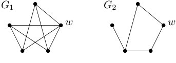 Figure 1
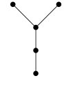 Figure 2
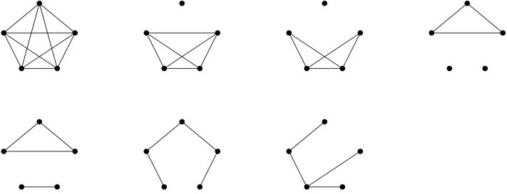 Figure 3
 Figure 4
Peer Reviews
No public reviews on file for this paper yet. If you reviewed it on a platform where reviews are public (OpenReview, ICLR, NeurIPS, ICML), you can paste yours below so the community can read it here.
Code & Models
Videos
No videos yet. Explain this paper in a talk, walkthrough, or lecture? Add one.
11footnotetext: Mathematics Institute and DIMAP, University of Warwick, Coventry CV4 7AL, UK22footnotetext: Department of Mathematics and Statistic, The Open University, Milton Keynes, MK7 6AA, UK33footnotetext: Department of Mathematics, Koç University, Saryer, Istanbul, 34450, Turkey
Strong Forms of Stability from Flag Algebra Calculations
Oleg Pikhurko1, Supported by ERC grant 306493 and EPSRC grant EP/K012045/1.
Jakub Sliačan*2,*111Part of this research was done when this author was supported by ERC grant 306493.
Konstantinos Tyros*3,*222Part of this research was done when this author was supported by ERC grant 306493.
Abstract
Given a hereditary family of admissible graphs and a function that linearly depends on the statistics of order- subgraphs in a graph , we consider the extremal problem of determining , the maximum of over all admissible graphs of order . We call the problem perfectly -stable for a graph if there is a constant such that every admissible graph of order can be made into a blow-up of by changing at most adjacencies. As special cases, this property describes all almost extremal graphs of order within edges and shows that every extremal graph of order is a blow-up of .
We develop general methods for establishing stability-type results from flag algebra computations and apply them to concrete examples. In fact, one of our sufficient conditions for perfect stability is stated in a way that allows automatic verification by a computer. This gives a unifying way to obtain computer-assisted proofs of many new results.
1 Introduction
By the term graph, we mean finite simple graph, that is, without loops and multiple edges. For a graph , we refer to the cardinality of its vertex set as the order of and we denote it by . Moreover, for a subset of the vertex set of , we denote by the subgraph induced by in , that is, the graph having as the vertex set and two nodes are connected in if and only if they are connected in .
Let and be graphs of orders . Call a subgraph of if there is a subset of such that is isomorphic to . (Thus a subgraph means an induced subgraph.) Let be the number of -subsets of that induce a subgraph isomorphic to . Also, let
[TABLE]
be the (induced) density of in ; equivalently, is the probability that a random -subset of induces a subgraph isomorphic to .
Suppose that we have a (possibly infinite) family of forbidden graphs. Call a graph admissible or -free (and denote this by ) if no is a subgraph of . Let be the family of all admissible graphs; clearly, is a hereditary graph property, that is, every subgraph of some member of belongs to , too.
Let be a positive integer. We denote by the set obtained by taking one representative from each isomorphism class of graphs in of order . Clearly is a finite set. Let be a function from to the reals. It gives rise to two other functions defined on graphs with :
[TABLE]
One can view as the expected value of , where is a random -subset of .
Under the above conventions, consider the problem of maximising over admissible graphs of given order . Namely, we define the extremal function
[TABLE]
and its density version . It is not hard to show (see Lemma 2.2) that the sequence is non-increasing and therefore the following limit exists:
[TABLE]
This is a rather general setting. As an illustration, here is one example (and the reader is encouraged to consult other concrete examples that can be found in Section 1.1).
Example 1.1** (Turán function)**
Let , and , where by we denote the complete graph of order and by the complement of a graph . (Thus is the number of edges in .) If is any family of graphs and consists of all graphs that can be obtained from by adding some missing edges, then is the well-known Turán function .
Fix a graph with vertex set . For pairwise disjoint sets (some of which may be empty), let the blow-up be obtained from the empty graph on by adding for every edge the complete bipartite graph with parts and . Note that no part spans an edge. Let be the family of all possible blow-ups of . It consists of graphs that can be obtained from by a sequence of vertex duplications and vertex deletions.
Suppose that . Trivially, we get the lower bound valid for every integer , where, in accordance with our general notation, is the maximum value of over all blow-ups of of order . For a vector in the -simplex
[TABLE]
define
[TABLE]
where for each . In other words, we look at the limiting value of the function evaluated on a blow-up of of order where the -th part occupies -fraction of all vertices. It is easy to see that the limit in (4) exists (and does not depend on the choice of the sizes ). In fact, is a polynomial in of degree at most , so the rate of convergence in (4) is . An easy argument based on the compactness of and the continuity of as a function of shows that
[TABLE]
By our assumption, so is a lower bound on .
Here is an illustration. In Example 1.1, if consists of the -clique, then a good choice is to take . Then is a subset of and . This is clearly maximised if all entries are equal to each other, giving , which is a lower bound on the Turán density of . The classical results of Mantel [28] (for ) and Turán [44] (for any ) imply that this is an equality. More strongly, they showed that for all , while an easy optimisation shows that is attained by the (unique) blow-up of of order with parts as equal as possible.
In general, there is no hope for a theory that allows to determine for every and . Namely, as it was shown by Hatami and Norin [22], the question if on input is undecidable in general (even if consists of all graphs). However, one can determine for various concrete examples of interest. Many of these proofs utilise the powerful flag algebra approach of Razborov [38, 40], where a computer can be used to generate a certificate proving .
We will discuss certificates in more detail in Section 3. For the time being, let us just remark that the desired inequality follows by symbolically representing , for as a sum of squares within error term of order as . One illustrative example of such a sum is , where is the degree of in a graph . Clearly, is non-negative while it is routine to see that , where is the path with vertices. This gives an asymptotic inequality that always holds between 3-vertex subgraph densities. One advantage of the flag algebra approach is that it allows us to generate and manipulate such equalities automatically; here finding optimal coefficients amounts to solving a certain semi-definite programme (which is independent of ). We refer the reader to Section 3 for details and formal definitions.
Thus, if a flag algebra calculation proves while we can find an order- graph with and with , then we know within an error term of :
[TABLE]
In addition to determining , it is often desirable to obtain information on the structure of all large admissible graphs for which the value is close to the maximal possible. In particular, we look for sufficient conditions establishing that every such is necessarily close to a blow-up of , in which case we regard the problem as stable. This paper will consider a few non-equivalent versions of stability, with the corresponding definitions following shortly. The stability is a very useful property in extremal graph theory as it is often indispensable in determining the exact value of as well as the set of all extremal graphs of large order . Besides being an important property on its own, stability also helps in solving the randomised or counting versions of extremal results.
We will use only one notion of distance on graphs. Namely, the (edit) distance between two graphs and of the same order is
[TABLE]
where the minimum is taken over all bijections . In other words, is the minimum number of adjacencies that one needs to change in in order to obtain a graph isomorphic to . We define the normalised (edit) distance to be . For a family of graphs we define and .
We say that our problem (2) is robustly -stable (resp. perfectly -stable) if there is such that for every graph of order we have
[TABLE]
(resp. ). For comparison, the classical -stability states that for every there is such that for every with vertices and . Clearly, the perfect stability implies the robust stability which in turn implies the classical stability. (Our Theorem 1.11 will in particular show that these notions of stability are not equivalent, already for such a natural problem as the Turán function.) Also, if the problem is perfectly stable, then for all we have and every extremal graph is a blow-up of (which one may call an exact result).
For example, for the Turán function , the classical stability was established independently by Erdős [10] and Simonovits [42]. The perfect (and thus also robust) stability in the case when consists of a clique follows from results of Füredi [15] (who considered the distance to being -partite instead of complete -partite as we do in this paper). Very recently, Roberts and Scott [41] improved on Füredi’s result by extending it to all colour critical graphs and giving a sharper bound on the distance.
As far as we know, the above results in [15, 41] and some recent work of Norin and Yepremyan [33, 34] (who considered the Turán problem for hypergraphs) are the only known examples where perfect stability was established for a non-trivial problem. Furthermore, almost all proofs where the classical stability and the exact result were derived from a flag algebra computation were rather ad-hoc and taylored to a particular problem.
The purpose of this paper is to present some general sufficient conditions that imply some version of stability. This allows us to give a unified proof of many previous stability and exactness results. Also, we can establish perfect stability (a new result) for a number of problems.
More specifically, Theorem 4.1 gives a sufficient condition for robust stability and Theorems 5.8, 5.13, and 7.1 give various sufficient conditions for perfect stability. Furthermore, all assumptions of Theorem 7.1 are stated in a way that allows automatic verification by a computer. We also present an openly available computer code (written in sage by adopting the flagmatic package of Emil Vaughan [45]) that allows us to both generate and verify certificates for general problems based on Theorem 7.1. In all the cases where we could verify assumptions of Theorem 7.1 and derive perfect stability, the procedure was essentially mechanical and the final high-level code is very short (having 6–10 lines, each invoking some function).
Even if one knows that for a concrete , the determination of asymptotically optimal part ratios (namely, finding all with ) may still be a non-trivial task that amounts to polynomial maximisation. While the combination of Lagrange multipliers and Gröbner bases provides a general computational framework, in an extremal problem one often has a candidate and wishes to prove that this is the only vector (up to a symmetry of ) that achieves . Clearly, if a flag algebra certificate proves that then this automatically implies that is a maximiser and it is possible that the information in is enough to imply the uniqueness of . We present such a sufficient condition on in Lemma 6.2 which can be automatically verified by a computer and seems to work very well in practice.
The exact statements of the above sufficient conditions rely on understanding flag algebra certificates, so we postpone them until later. Here, let us list the extremal problems for which our method gives perfect stability. In almost all cases, Theorem 7.1 and Lemma 6.2 apply directly, immediately giving perfect stability and implying the uniqueness of asymptotically optimal part ratios.
However, there are a few natural problems where the assumptions of Theorem 7.1 are not satisfied. As the test case that our method can still give perfect stability, we chose the inducibility function for the paw graph, see Theorem 1.10. The asymptotic value of this function was determined by Hirst [24] but the classical stability and the exact result were not known. By utilising our other results (Theorem 5.8) we derive perfect stability for the inducibility problem for the paw graph. Since the proof is rather long and was meant mainly as an illustration of the flexibility of our method, we decided to include only one such example in this paper.
1.1 Examples of extremal problems for which we can prove perfect
stability
1.1.1 Minimising the number of independent sets in
triangle-free graphs
Erdős [9] asked for the value of , the minimum number of independent sets of size in a -free graph of order .
Consider first the case , when we forbid a triangle. Goodman [17] determined ; his bounds also give the asymptotic value of . Lorden [26] showed that, for , the value of is attained by taking and removing any (possibly empty) matching from it. Some partial results were obtained by Nikoforov [32, 31]. The problem for remained open until recently when the classical stability and the exact result were established independently by Das, Huang, Ma, Naves and Sudakov [7] (for ) and Pikhurko and Vaughan [36] (for ) when is sufficiently large: if , then all extremal graphs are blow-ups of and if , then all extremal graphs are blow-ups of the Clebsch graph . The Clebsch graph has, as vertices, binary -sequences of even weight (that is, the number of ones), with two vertices being adjacent if the point-wise sum modulo 2 of the corresponding sequences has weight . It easily follows from this description that the graph has 16 vertices and is triangle-free and -regular.
This question of Erdős is a special case of our general problem. It turns out that our computer codes can prove the perfect stability in the following cases. (Note that the -problem is not perfectly stable by the above mentioned result of Lorden [26].)
Theorem 1.2
Let
- •
* and , or*
- •
* and .*
Let (thus consist of all triangle-free graphs) and let be 0 except . Then the corresponding problem (that is, Erdős’ problem of determining ) is perfectly -stable. Furthermore, for each the unique probability vector that maximises is the uniform vector.
If , then the asymptotic value of is known only for and , see [7, 36]. The papers [7, 36] also showed that in each of these cases the problem is classically -stable, where , and the value of is attained by a blow-up of for all large . However, the problem is not perfectly -stable since it is possible to remove a few edges from the blow-up of (e.g. a matching between two parts) so that the number of copies of does not change.
The above results and our Theorem 5.13 imply that, in fact, the -problem is not robustly stable for . Alternatively, the same conclusion can be derived directly by taking the optimal blow-up , fixing some sets and each of size , where is a small constant, and then flipping all pairs between and . (Such tranformation is done in the proof of Theorem 5.13 and is carefully analysed there.)
1.1.2 Maximising the number of pentagons in triangle-free graphs
Erdős [11] asked if for every natural number , where is the maximum number of 5-cycles that a triangle-free graph of order can have. Note that this bound is sharp for every which is witnessed by the balanced blow-up of .
Some partial progress on this problem was obtained by Győri [19] who proved and Füredi (unpublished) who proved . Recently, Grzesik [18] and independently Hatami et al. [21] proved that, as , there can be at most copies of . Furthermore, Hatami et al. [21] proved the exact result for all large (and the classical stability can also be derived from their method). In fact, the validity of Erdős’ conjecture follows from the asymptotic result by a simple blow-up trick (see [21, Corollary 3.3]). Interestingly, if , there is another extremal example which is not a blow-up of that was discovered by Michael [29]. Very recently, the value of and the description of all extremal graphs for every was obtained by Lidický and Pfender [25].
This problem fits into our general framework and we can prove (again in a completely automated way) that it is perfectly stable.
Theorem 1.3
Let , , and be zero, except . Let . Then the corresponding problem is perfectly -stable (with the unique maximiser for being the vector with each entry equal to ).
1.1.3 Inducibility
Given a graph , the inducibility problem for asks for the maximal possible (induced) density of the graph among all graphs of order . In our general notation, it can be expressed as follows. Let , and let take the value 0 on every graph with vertices except , where it takes value 1. Thus we are interested in . We call the inducibility of . Equivalently,
[TABLE]
Observe that the inducibility of each graph is equal to the inducibility of its complement. The inducibility problem has drawn a considerable amount of interest, see for example [2, 3, 4, 6, 13, 14, 16, 20, 23, 24, 43].
Before we look at concrete examples, let us mention the following general result of Brown and Sidorenko [6, Proposition 1]: if is complete partite (i.e. a blow-up of some clique), then for every at least one -extremal graph is complete partite. The proof in [6] uses the symmetrisation method and it is not clear how to extract a stability-type result from it. Also, Even-Zohar and Linial [13, Table 2] systematically looked at the inducibility of 5-vertex graphs but without trying to convert the numerical bounds coming from flag algebra calculations into computer-verifiable mathematical proofs.
1.1.4 Inducibility of the cycle on four vertices
The inducibility of the 4-cycle, denoted by , follows from the above mentioned result of Brown and Sidorenko [6]. Previously, Pippenger and Golumbic [16] determined for all with , observing that the complete balanced bipartite graph is an extremal graph. Here we prove perfect stability for this problem (by invoking our computer code).
Theorem 1.4
Let , , and be zero, except . Let be a single edge. Then the corresponding problem is perfectly -stable (with and the unique maximiser for being the vector ).
1.1.5 Inducibility of minus an edge
Let be the graph obtained by removing an edge from the complete graph on four vertices. The inducibility problem for was considered by Hirst [24], who determined using the flag algebra method. Our new result is that this problem is perfectly stable (and, in particular, that is attained by a blow-up of the complete graph on five vertices , for all large ).
Theorem 1.5
Let , , and be zero, except . Also let . Then the corresponding problem is perfectly -stable (with and the unique maximiser for being the vector with each entry equal to ).
1.1.6 Inducibility of
The function was calculated by Golumbic and Pippenger in [16], where the complete balanced bipartite graph is an extremal graph. We show that the problem is perfectly stable.
Theorem 1.6
Let , , and be zero, except . Also let . Then the corresponding problem is perfectly -stable (with and the unique maximiser for being the vector ).
1.1.7 Inducibility of
The function can be derived from the results of Brown and Sidorenko [6]. Here we prove perfect stability for the corresponding problem.
Theorem 1.7
Let , , and be zero, except . Also let . Then the corresponding problem is perfectly -stable (with and the unique maximiser for being the vector ).
1.1.8 Inducibility of
We consider the inducibility problem for the disjoint union of a path on 3 vertices and an edge, which we denote by . We prove the following.
Theorem 1.8
Let , , and be zero, except . Also let , that is, the disjoint union of two triangles. Then the corresponding problem is perfectly -stable (with and the unique maximiser for being the vector with each entry equal to ).
1.1.9 Inducibility of the “Y” graph
We consider the inducibility problem for the graph depicted in Figure 1, which we denote by . We prove the following.
Theorem 1.9
Let , , and be zero, except . Also let . Then the corresponding problem is perfectly -stable (with and the unique maximiser for being the vector with each entry equal to ).
1.1.10 Inducibility for the paw graph
Let us denote by the graph obtained by adding to a triangle a pendant edge. Using flag algebras, Hirst [24] determinend the value of . Here, it is more convenient to work with the (equivalent) complementary problem. Thus we consider the inducibility problem of the disjoint union of a path on three vertices and a single node, that we denote by . Unfortunately, the perfect stability does not follow directly from Theorem 7.1. However, it can be proved using our methods combined with additional work, see Section 8.1 for the proof.
Theorem 1.10
Let , , and be zero, except . Also let , that is, the disjoint union of two edges. Then the corresponding problem is perfectly -stable (with and the unique maximiser for being the vector with each entry equal to ).
1.1.11 Turán problem
Recall that the Turán problem was introduced in Example 1.1. Given a family of graphs we consider , the collection of graphs obtained by adding missing edges to the graphs in . While our computer code can automatically prove the perfect stability when with , this is superceded by the following result whose proof does not require a computer. For integer denote by the balanced blow up of on vertices (i.e. with ).
Theorem 1.11
Let be a family of graphs and let
[TABLE]
where by we denote the chromatic number of the graph , that is, the minimum number of colours needed in a coloring of the vertex set with no adjacent vertices of the same colour. Then the following hold.
The Turán problem is perfectly -stable if and only if there is an integer such that plus one edge is not -free. 2. 2.
*Assuming in addition that is finite, we have the following. The Turán problem is robustly -stable if and only if there is an integer such that plus some forest in one of the parts of is not -free. *
As we learned later, the non-trivial implication in Part 1 of the above theorem is apparently a folklore result. Since it follows from [41, Lemma 2.3], we omit its proof. The second part of Theorem 1.11 is proved in Section 9 of this paper.
2 Notation and preliminaries
Some of the definitions and proofs of this paper will be more natural when stated in a more analytic way. For example, the definition of in (4) would not require a limit if instead we were working with vertex-weighted graphs. Such objects are quite common in extremal graph theory nowadays (appearing, for example, in the definition of the Lagrangian of a graph that goes back to Motzkin and Straus [30]) and, of course, they are generalised in a powerful and far-reaching way by graphons (see, for example, the excellent book by Lovász [27]). However, we believe that by staying within the universe of simple unweighted graphs, we make the paper and its ideas better accessible to a wider audience.
As usual, for each positive integer , we denote by the set . Let denote the expected value of a random variable . We will often abbreviate a pair as . For a finite set and a positive integer we denote by the set of all -subsets of .
Recall that denotes the complete graph of order and denotes the complement of a graph . Let be the complete bipartite graph with part sizes and . For a vertex , let denote the neighbourhood of in . We write if and are isomorphic graphs.
We call a graph -minimal if strictly decreases when we remove any vertex of . By (5), is -minimal if and only if no point on the boundary of achieves the maximum.
A graph is twin-free if it contains no two vertices and with identical neighbourhoods (i.e., for all distinct we have ).
Recall that the (edit) distance between two graphs and of the same order is the minimum of adjacencies one has to edit in to make it isomorphic to . Also, the (edit) distance from a graph to a family of graphs is the minimum of over all that have the same order as ; this is the minimum number of adjacency edits needed to transform into a graph in . The respective normalised distances are and .
Throughout this paper we will work under the following assumptions which are collected together for future reference.
Assumption 2.1
Let be positive integers and a family of graphs.
Set . 2. 2.
Let be a function and define and as in (1). 3. 3.
*Let be a graph on such that . *
The next lemma provides some basic information on the behaviour of the sequence .
Lemma 2.2
Let be a graph property closed under taking induced subgraphs. Then for with we have
[TABLE]
Furthermore, if is closed under taking blow-ups, then the error term is .
Proof. Take an optimal graph for . Let be a random -subset of and . Then . Thus . Clearly, if we take a uniform and then a uniform , then is uniformly distributed among all -subsets of . Thus equals , giving . Thus is non-increasing in and tends to a limit, implying the other desired inequality .
Finally, assume that is also closed under taking blow-ups. To show , take an optimal graph for on . Consider a random map with all choices being equally likely and let be the graph on with . Take any -subset . With probability , the map is injective on . If we condition on this, then is uniform and the average of is . Thus
[TABLE]
giving the desired.
3 Flag algebra method
As we have already mentioned in the introduction of this paper, the flag algebra method is a powerful technique pioneered by Razborov [38, 40]. In this section, we define what a certificate is and how it implies an upper bound on . Recall that we always work under Assumption 2.1.
3.1 Types and flags
A type is a pair of the form , where is an admissible graph and is a bijection with . Given a type as above, a -flag is a pair of the form , where is an admissible graph and is an injection such that is an embedding (that is, an injection that preserves both edges and non-edges). Informally, a -flag is a partially labelled graph such that the labelled vertices induce . The order of the flag is , the number of vertices in it.
For two -flags and with respectively vertices, let the sub-flag count be the number of -subsets of such that (i.e. contains all labelled vertices) and the -flags and are isomorphic, meaning that there is a graph isomorphism that preserves the labels. Also, define the (flag) density as
[TABLE]
The latter quantity can be viewed as the probability that a random -subset of with induces a copy of the flag in .
We will also need a variation of the above notion. Let , and be three -flags with respectively and vertices. We define the joint sub-flag count to be the number of pairs such that are subsets of with and elements respectively, and the -flags and are isomorphic to and , respectively.
The type with no vertices will be denoted by 0. Thus [math]-flags are just unlabelled graphs. In this case, the 0-flag density as defined by (6) coincides with the notion of subgraph density from the Introduction.
3.2 Certificates
Definition 3.1
A (flag algebra) certificate is a triple
[TABLE]
where
- •
* is an integer;*
- •
* is an ordered list of some types such that is a positive even integer for each ;*
- •
* is an arbitrary positive semi-definite -matrix for , where we fix some enumeration of all -flags with exactly vertices, up to isomorphism of flags (and thus is the number of these flags).*
Note that the third component of the certificate consists of exactly matrices, one per each of the types ; one can view the rows/columns of as indexed by the -flags of order .
To describe the upper bound of that a certificate witnesses, we need to introduce several quantities.
Let be the enumeration in some fixed order of all (up to an isomorphism) admissible -vertex graphs. Thus with no two listed graphs being isomorphic. For each (that is, for each ), we define real numbers
[TABLE]
and the sum in the definition of is taken over all injective maps that induce a copy of the flag in . Also, let
[TABLE]
and
[TABLE]
A graph is called -sharp (or -sharp, or just sharp) if . The following lemma motivates the above definitions.
Lemma 3.2
Under the above notation, for every admissible graph of order we have that
[TABLE]
In particular, we have that and .
Proof. Let be an arbitrary admissible graph of order . We have
[TABLE]
proving (9).
Next, we define a non-negative quantity in the following way. Initially, we set . For each non-negative integer such that is a positive even integer we work as follows. We enumerate all injections . If the induced type is equal to some , then we add the quantity to , where
[TABLE]
Since each matrix is positive semi-definite, we have that each and that the final is non-negative.
Let and set . Take any . Notice that the sum of the products over all injections such that is isomorphic to , is equal to
[TABLE]
where is defined in (8), see e.g. [38, Lemma 2.3]. (Informally speaking, we just count in two different ways the number of embeddings of and into so that the correponding labelled vertices coincide; the error term comes from embeddings where some unlabelled vertices happen to collide.) Thus, summing over , as well as, over injections and expanding each quadratic form , we get the representation
[TABLE]
where ’s are as in (8). Adding this to (11), we obtain that
[TABLE]
The inequalities in (10) follows readily by (13) and (14).
Lemmas 2.2 and 3.2 have the following immediate consequence.
Corollary 3.3
*Suppose that Assumption 2.1 holds. Let be a vector in and a certificate such that . Then . Moreover, if is closed under taking blow-ups, then . *
Finally, we close this section with the following lemma.
Lemma 3.4
Under Assumption 2.1, suppose that is closed under taking blow-ups and that a certificate and a vector with no zero entry satisfy . Fix and set . Also, let be a large positive integer, a partition of with and . Finally, let be an injection such that is a -flag. Define as in (12). Then .
Proof. Observe that any modification of the injection such that its values stay in the same parts is an embedding. These new injections give the same vector . There are such injections since each part has size . Let be the quantity defined in the proof of Lemma 3.2 when applied to . Note that is the sum of non-negative quantities, some of which correspond to the above embeddings of into . Thus
[TABLE]
Also, observe that . Since , by (10) and (13) we have that . Invoking (15), the result follows.
4 Robust stability from flag algebra proofs
The main result of this section is Theorem 4.1 below that provides a sufficient condition for a problem to be robustly stable. Let be two graphs. We say that a map is a strong homomorphism if it preserves both adjacency and non-adjacency. Observe that a strong homomorphism, in contrast to an embedding, does not need to be injective, allowing pairwise non-adjacent vertices to be mapped to the same image. Moreover, let us note that a graph admits a strong homomorphism in a graph if and only if is a blow-up of .
Theorem 4.1** (Robust Stability)**
Suppose that in addition to Assumption 2.1 the following holds.
*We have a vector and a certificate with . * 2. 2.
There is a graph of order at most satisfying the following.
- (a)
. 2. (b)
There exists a unique (up to automorphisms of and ) strong homomorphism from into . 3. (c)
For every distinct and in we have . 3. 3.
Every -sharp graph of order admits a strong homomorphism into .
Then the problem is robustly -stable.
Proof. By Corollary 3.3, we know that . For notational convenience, assume that . Choose large constants in the order . In particular, we assume that . Take any -free graph of order . Note that Condition 2(c) of Theorem 4.1 implies that is twin-free.
We can assume that for otherwise
[TABLE]
and there is nothing to do. Since is -free but is strictly larger than , the supersaturation argument of Erdős and Simonovits [12] or an application of the Removal Lemma shows that
[TABLE]
that is, has at least copies of .
For every embedding , we define the following. For each binary string of length , let consist of those vertices such that the neighbourhood of in is given by , that is, . Thus, the sets , , form a partition of . Observe that, if we apply the above definition to the (fixed) map (instead of ), then each part in the obtained partition of has at most one vertex by Condition 2. Let be the binary sequence corresponding to the part for each ; thus encodes the adjacencies of to the fixed copy of in . We call all other length- binary sequences singular. Also, we call a part singular if is singular, that is, not one of . Finally, we call a pair of distinct vertices singular if at least one of them is in a singular part or both of them are in non-singular parts but the adjacency relations between in and between in mismatch (that is, one is an edge and the other is a non-edge), where is the unique element of satisfying for . Note if we have above, then is singular if and only if and are connected in .
Observe that due to Condition 2, we have that the union of with every singular pair induces a graph that does not embed into a blow-up of . For example, if is in a singular part then already spans a subgraph in that does not belong to . If we add an arbitrary disjoint -set of vertices to , we get a subgraph of of order that does not belong to . Condition 3 and inequality (10) give that the total number of such subgraphs in is at most , where we assume that is smaller than . Also, each such subgraph of can arise for at most triples , a rough bound on the number of ways to embed into , then choose two more vertices in and let be the rest of . Thus, the number of triples as above is at most . Clearly, if we fix the first two entries, namely , then any choice of will do and there are at least choices of (as is always at most ). Thus the total number of possible choices of as above is at most
[TABLE]
Choose for which the number of singular pairs is at most the average. By (16) and Corollary 3.3, it is at most
[TABLE]
Observe that one can convert into a blow-up of by flipping all singular pairs between non-singular parts of and merging the singular parts into non-singular ones in an arbitrary way. Thus, for every (and in particular this) , the number of singular pairs is at least , which is by definition the minimum number of pairs that one needs to change in to make is a blow-up of . This finishes the proof of the theorem.
5 Sufficient conditions for perfect stability
The aim of this section is to present sufficient conditions for perfect stability. To state our results, we need the notions of strictness and flip-aversion. Their definitions require several other concepts that we introduce in the next section.
5.1 Notation and some preliminary results
Throughout this section we work under the following set of assumptions.
Assumption 5.1
In addition to Assumption 2.1, we assume the following.
Each graph in is twin-free and 2. 2.
.
Observe that a trivial consequence of twin-freeness of each is the following.
Lemma 5.2
*The set of admissible graphs is closed under taking blow-ups. *
We will also need the following pieces of notation. If is a graph and is a pair of distinct nodes of , then by we denote the graph obtained by flipping the adjacency of and , while by we denote the graph obtained by deleting the node in . Moreover, if is a positive integer, for a graph of order and a vertex of , we define
[TABLE]
The value of can be determined by summing over all -subsets of containing . Also, is the conditional expectation of where is a random -subset of conditioned on .
Let in be arbitrary. Consider a blow-up of order , where . Let be obtained from it by adding a new vertex . Then is determined within additive error by the vector of ratios
[TABLE]
In fact, we have
[TABLE]
where is some real polynomial in . One can write explicitly as follows.
First, for a (not necessarily injective) map and a (binary) vector in , let be the graph on such that two elements and of are adjacent if and only if and are adjacent in , and is an edge if and only if . Informally speaking, is a graph that we can form from a blow-up of on by adding a new vertex whose neighbourhood in is given by the binary vector . Then the value of the polynomial at is
[TABLE]
Let us call a vector admissible if for every , every map , and every binary vector such that implies and implies (while can be arbitrary if ), the graph is -free. In other words, this condition says that if we take a blow-up with each large and add a vertex with neighbours in for each , then the obtained graph is still -free. Clearly, whether is admissible or not, depends only on the sets and and therefore the next claim follows easily.
Claim 5.3
*The set of the admissible vectors forms a closed subset of . *
Let us point out that, since is twin-free, it suffices to check the condition in the definition of an admissible only for those choices of for which is twin-free. In particular, it suffices to consider to be at most .
The following vectors will play a special role. For every , we define in by setting if belongs to and otherwise for all . Informally speaking, the assignment corresponds to adding one extra vertex in part . Thus each vector is admissible. Under this terminology, we have, in particular, for each and that
[TABLE]
Indeed, both sides of (20) measure the (normalised) change in the objective function when we remove one vertex from the -th part of an -blow-up of of order .
There is the following connection between and .
Claim 5.4
[TABLE]
Proof. First, for every positive integer and map we define to be the graph having as the vertex set with and being adjacent if and only if and are adjacent. For each we define
[TABLE]
and
[TABLE]
Then we have that
[TABLE]
On the other hand, we have that
[TABLE]
Let us illustrate some of the above concepts in the special case of Example 1.1 with (namely, the Turán function ). Here and . Ignoring rounding errors, if we create from the complete -partite graph by adding a new vertex having neighbours in respectively, then is just , the number of edges at . Thus . Since we forbid , a vector is admissible if and only if at least one is 0. Here is the -vector corresponding to being a twin of the vertices in , that is, consists of 1s except one 0 at position . Note that is the (unique) maximiser of for . If we fix this and maximise over admissible , then trivially the set of maximisers is . The following lemma states that one part of this inclusion (namely, that each is a maximiser) holds whenever has no zero entries. This makes a perfect combinatorial sense: in every extremal configuration all vertices must make asymptotically the same contribution to .
Lemma 5.5
Fix any that maximises . Suppose that has no zero entries. Then the maximum of over admissible is and, furthermore, for each (that is, each of the vectors is a maximiser).
Proof. Since achieves a maximum and lies in the interior of , we have that for all . Denote this common value by . By Claim 5.4, we have for all . Since is a homogeneous polynomial of degree , we have that
[TABLE]
This, the fact that maximises , Claim 5.4, and equality imply that
[TABLE]
Thus for all .
To prove the first part of the lemma, we derive a contradiction by assuming that some admissible achieves a strictly greater value. Let and pick some real with .
Here we can start with of order with and form by adding a set of new vertices that span an independent set with the identical adjacencies to governed by . Since the vector is admissible, the obtained graph is -free. Indeed, plus one vertex is -free by the admissibility of ; by blowing up the vertex we cannot violate -freeness because each member of is twin-free.
The contribution of the new vertices to is . Indeed, if we take a random -subset of , then with probabilities respectively , , and , the set intersects in zero, one and at least two vertices; thus
[TABLE]
So we see that can be made strictly positive by choosing small constant . Thus the -blow-up of is not asymptotically optimal, contradicting the optimality of .
Let us say that is -strict if the set of maximisers of over the admissible ’s in is exactly . Call the graph -strict if is -minimal and is -strict for every that maximises .
Recall that is -minimal if is strictly smaller than for any proper subgraph of . It trivially follows that such is necessarily twin-free and every maximiser has all coordinates non-zero (and by compactness at least one maximiser exists). Thus, if is -strict, then, for each optimal , each of is a maximiser of by Lemma 5.5 while the strictness property requires that there are no other maximisers.
Lemma 5.6
If is -strict, then for every there is such that if and admissible satisfy and , then is -close to some .
Proof. Suppose there is that violates the lemma, that is, for every there are and that violate the conclusion for . By passing to a subsequence, we may assume that these vectors converge to and respectively. By the continuity of , is a maximiser. By -minimality of we have that each . By Claim 5.3, we have that is admissible, while by Lemma 5.5 and Assumption 5.1 we have that . Since is -strict, we have that is equal to for some . But then has to get -close to leading to a contradiction.
Here is another easy consequence of the compactness of .
Lemma 5.7
*If is -minimal, then there is such that for every satisfying we have that each is at least . *
Finally, we call a graph -flip-averse if there is such that the following holds. If we take a blow-up with vertices such that and obtain by changing the adjacency between a pair of distinct nodes (possibly from the same part), then either contains some with as a subgraph or we have that
[TABLE]
By compactness, the property of being flip-averse can be equivalently re-formulated in terms of the polynomial , where disappears from the definition but then its combinatorial meaning will be less clear.
5.2 Main results for perfect stability.
This section consists of two results, each providing a sufficient condition for perfect stability. The first one is the following.
Theorem 5.8** (Perfect Stability I)**
Suppose that, in addition to Assumptions 2.1 and 5.1, the following assumptions hold.
The problem is classically -stable. 2. 2.
The graph is -strict. 3. 3.
The graph is -flip-averse.
*Then the problem is perfectly -stable. *
Proof. Given , we fix sufficiently small positive constants .
To prove the perfect stability we pick some large enough real number (depending on the previous constants). In this proof, let asymptotic notation such as or hide constants that depend on , , , and only (but not on the constants ).
Let be an integer with . Choosing large enough, we may assume that . Let be an arbitrary admissible graph on . Assume that for otherwise the result follows trivially, since and the normalised distance is always bounded by . By Condition 1, that is, the classical -stability, there is a partition such that
[TABLE]
where and . We call pairs in wrong. Assume that the parts were chosen so that is minimum. Clearly, this choice of parts implies that (23) still holds. Since the number of -subsets of such that is at most , we conclude that
[TABLE]
where .
Let us call a vertex special if . We set to be the set of special vertices and .
For each , we set . By (24), the continuity of , and the compactness of , we can assume that the vector is -close to a maximiser of , that is,
[TABLE]
By Lemma 5.7, we can assume that each ; thus we conclude that for each .
At this point, we can give an informal overview of the rest of the proof. First, Claim 5.9 shows that, for every vertex of , the normalised contribution of a vertex to is less than for otherwise the addition of an appropriate number of clones of to will bring well over , which is impossible. It follows that, in order to avoid being too small, we have that . Furthermore, the adjacenty of each vertex essentially follows the ideal adjacency of part- vertices, for some , as this is the only possibility to have close to by the assumed -strictness. Since our choice of the parts minimises the number of wrong adjacencies, this vertex has to belong to and thus its wrong degree is necessarily small, see (29). (Also, somewhat conversely, each vertex has high wrong degree, just to account for the drop .) This, the near-optimality of , the fact that is small and the -flip-aversion give that every edge-flip inside has negative effect on (Claim 5.11), not only with respect to but also with respect an arbitrary graph obtained from by changing some adjacencies inside (Claim 5.12). Thus if we flip , all wrong pairs outside , and “fix” each vertex of , then increases by at least per one changed edge. (Note that, since all vertices of high -degree are inside the small set , the “pairwise” effects can be shown to be negligible.) On the other hand, is clearly an upper bound on the edit distance from to the family . These two estimates give the perfect stability.
Let us provide all the remaining details now.
Claim 5.9
For every vertex , we have that .
Proof of Claim. We assume on the contrary that there exists a node satisfying . Set . Consider obtained from by adding clones of . We view as the expectation of for a random -set . With probability at least , the set is disjoint from the added clones and its conditional expectation is exactly . With probability , the set has exactly one element from the added clones and avoids . Conditioned on the latter event, is the same as where we take a random -subset of conditioned on ; thus the conditional expectation of is exactly (which we assumed to be at least ). Finally, the contribution from the remaining sets is in the absolute value at most times their probability . Also, note our choice of such that . Thus
[TABLE]
This is strictly larger than . On the other hand, by Lemma 5.2, we have that is admissible and therefore, invoking Lemma 2.2, we get that , a contradiction.
If we pick a uniform random , then the difference is never below by Claim 5.9, while with probability it is at least . On the other hand, the average of over is . Thus and, roughly, .
Take any . Let be obtained from by changing adjacencies at so that . We have that , where is an element of defined by for all . We also define another element of by setting unless if (resp. ), then we set (resp. . Clearly,
[TABLE]
Claim 5.10
The vector is admissible.
Proof of Claim. Suppose that the claim does not hold. Let this be witnessed by a vector and a map . Then implies , while the graph is of order and not -free. As we observed after the definition of an admissible vector, one can assume that . If does not belong to , then is -far from [math] and . Also, we know that each has at least vertices.
Let us show that has at least copies of via . In fact, it is enough to consider only the copies where the vertex of is mapped into . For , let be if and if ; note that always has at least vertices. Now, if we map each arbitrarily into , then these vertices together with form a copy of in , giving at least the stated number of copies.
Each of the above copies contains a wrong pair which is not adjacent to . (Recall that is -free but is not and that the vertex has the same neighbourhoods in and .) On the other hand, each wrong pair disjoint from can be counted at most times. This gives at least wrong pairs, contradicting (23) since is sufficiently small with respect to and (and ).
By (25) we also have that . On the other hand, there are at most -subsets of satisfying and , because each such set must contain a wrong pair disjoint from . Thus by (23), we have that . Also, observe that . By (26), we get that . By the Triangle Inequality, we derive that
[TABLE]
Suppose furthermore that . By the definition of , we have that and therefore
[TABLE]
By Assumption 2, Lemma 5.6 and Inequality (27), we conclude that is -close (in the -norm) to the “adjacency vector” of some . By (26),
[TABLE]
Next, let us show that belongs to . Suppose on the contrary that belongs to for some . By the twin-freeness of (which trivially follows from the -minimality of ), there is some which is adjacent to exactly one of and , say but . The vertex is adjacent in to vertices of . But we know that and, by (28), . On the other hand, has no edges between and . Thus belongs to at least wrong pairs having an endpoint in . Let as denote this set of edges by . Consider changing the partition by moving to . Observe that the new set of wrong pairs will differ from the old one only on edges containing . By (28), at most edges can be introduced into the set of wrong pairs, while every edge in will not be contained, anymore, in the new set of wrong pairs. Thus the number of wrong pairs will strictly decrease. This contradicts the choice of the partition and, in particular, the minimality of . Thus indeed , as claimed.
Thus, again by (28), we have that
[TABLE]
Claim 5.11
For every pair in , the graph (which is obtained from by changing the adjacency of ) is -free and satisfies .
Proof of Claim. Suppose on the contrary that contains a forbidden subgraph . Since consists of twin-free graphs and has at most pairwise non-twin vertices, we can assume that has vertices. In fact, we must have at least copies of on via in , since for each . Notice that the vertex set of each such copy contains a pair from different from . By (29), we have at most wrong pairs adjacent to , each in at most copies of ; while every other wrong pair appears in at most copies of . This gives that the total number of -subgraphs on via is at most
[TABLE]
where we used (23). This is strictly less than , a contradiction. This contradiction shows that no such exists, proving the first part of the claim.
The second part follow from Assumption 3 of the theorem.
Claim 5.12
Let be an arbitrary (not necessarily -free) graph having as a vertex set and such that , where . Then for every pair in we have
[TABLE]
Proof of Claim. Let us estimate , where we define
[TABLE]
Let be a -subset of that contributes different amounts to and . Clearly, both and belong to ; also has to contain at least one further pair . The number of the -subsets containing a pair satisfying is at most (the number of choices of ) times (the number of choices of ). Likewise, the number of the -subsets containing a pair satisfying is at most the number of wrong pairs adjacent to or , which by (29) satisfies
[TABLE]
times . Thus, (23) gives that . On the other hand, the sum
[TABLE]
has at most non-zero terms (all such have to contain the pair as well as intersect ). Observe that is at least by Claim 5.11. Thus , as desired.
Enumerate as . Let and for , let ; that is, we flip the wrong pairs on in some order. The final graph coincides with on . By using Claim 5.12 to estimate the effect of each of the flips, we conclude that
[TABLE]
On the other hand, we have that
[TABLE]
For each vertex , the value is at most by the definition of . By Claim 5.4, the value is equal to where is the index of the part that contains . Since is -close to an optimal vector (namely, a vector that satisfies ), we have that
[TABLE]
Thus for each and invoking (31) and (32), we get
[TABLE]
By (33) (and our bounds on and ), we have that, for example,
[TABLE]
Observing that and , we derive the perfect stability.
Theorem 5.13** (Perfect Stability II)**
Suppose that Assumptions 2.1 and 5.1 are satisfied, the problem is robustly -stable and is -minimal. Then the problem is perfectly -stable.
Proof. Clearly, the perfect stability will follow by Theorem 5.8 if we show that its Assumptions 1, 2 and 3 are satisfied. Assuming that the problem is robustly -stable, we trivially have that the problem is classically -stable, that is, Assumptions 1 of Theorem 5.8 is satisfied. Thus it is enough to verify Assumptions 2 and 3 of Theorem 5.8.
Roughly speaking, our proof is based on the following idea. For example, suppose that Assumption 2 (the strictness of ) fails. Let this be witnessed by a vector . Then we take a blow-up of order with optimal part ratios and add a set of twin vertices, each attached to according to . Since is -far from each canonical attachment , the new graph has normalised edit distance to the family . On the other hand, if we take a random -subset then it either is disjoint from (and the conditional expectation of is exactly ), or contains exactly one vertex of (and the conditional expectation of is by the choice of ), or contains at least two vertices of (which has probability ). We conclude that , a contradiction to the robust stability. Likewise, if some edge flip violates Assumption 3 (the flip aversion of ), then one “magnifies” this by flipping all pairs between two appropriately placed sets of size .
Let us continue with the formal proof. Let the robust stability of the problem be satisfied with constant . Given , and , we choose a small enough quantity .
In order to prove that the problem is strict, we assume on the contrary that there exist a maximiser in of and an admissible in violating -strictness. Since is -minimal, we have that each . We set
[TABLE]
and we pick some positive real satisfying .
Let be a blow-up on vertices with . Let be obtained from by adding a set of twins whose attachment to is given by the vector , where we insist that if (resp. ), then each is adjacent to no vertex in (resp. every vertex in ). Since is admissible and the graphs in are twin-free, is -free. Since , we have that the average of over the -subsets of with is . Thus it follows that is at most . By robust stability, the normalised distance from to some blow-up of is . Clearly, .
Recall that we have partitions . We have that each for otherwise we obtain the contradiction that
[TABLE]
where is the maximum of over all blow-ups of proper subgraphs of . Similarly, each has at least elements.
Claim 5.14
There is an automorphism of such that for each
[TABLE]
Proof of Claim. We show first that for each there exists satisfying (34) (and then observe that the map is an automorphism of ). Take any . Suppose that there is no choice of satisfying (34). We pick such that . We distinguish the following two cases.
Case I: There exists such that and .
Since is twin-free (which follows by the -minimality of ), pick such that exactly one of is a -neighbour of . Then, every is incident to at least pairs on which the graphs and differ, because each has different -adjacencies to and but the same -adjacency to all vertices of . Thus which is not , a contradiction.
Case II: For every such that we have that .
It holds that . Since we work under the assumption that there is no appropriate choice of , we have, in particular, that and therefore . We pick with such that . Arguments similar to the ones used in Case I lead to a contradiction.
To complete the proof we show that is an automorphism of . Let us observe that is an injection. Indeed, suppose on the contrary that there exist and in such that and . Then we have that
[TABLE]
contradicting (34). To prove that is edge and non-edge preserving, we assume on the contrary that there exists a pair of nodes such that does not preserve adjacency. Then the graphs and differ on every pair with and generating at least such pairs. The latter is a contradiction to . The claim is proved.
By relabelling , we can assume that the bijection of Claim 5.14 is the identity map. We expand to a partition of the vertex set of setting for each . Clearly
[TABLE]
for all . Finally, we set
[TABLE]
Each vertex is adjacent to at least pairs in , because is -far from , and at most pairs in . Thus the symmetric difference between and is at least , a contradiction which shows that the graph is -strict.
Next, let us prove the -flip-aversion of . We pick some positive real and towards a contradiction we assume that there exists some integer with , an almost optimal blow-up on and some pair of distinct nodes such that the graph contains no forbidden graph of order at most and
[TABLE]
Let be such that and . We pick subsets and of and respectively with cardinality each. If then we choose and to be disjoint. Let be the set of all pairs of nodes with one node in and one in . Also let be the graph obtained by flipping the adjacency between each pair in . Since each of and consists of twins, does not contain any forbidden subgraph.
Let us show that
[TABLE]
Indeed, let be the set of all -element subsets of . We partition into , and , the set of all containing respectively zero, one and at least two pairs of . Finally, for each , we set , and to be the set of all , and respectively, containing . Note that if , then and thus . We are going to use this fact a couple of times in the following chain of equalities.
[TABLE]
Therefore, by the almost-optimality of we have that . By the assumed robust stability, there exists some blow-up of such that . Following arguments as in the proof of Claim 5.14, we can assume that for every .
Then we distinguish the following three (non-exclusive) cases.
- (i)
. 2. (ii)
. 3. (iii)
and
We complete the proof by showing that each case leads to a contradiction and, in particular, we show that each case yields that . Indeed, let us assume (i). Then there is such that . Pick such that the -adjacencies of and differ. We have at least vertices in . Thus the symmetric difference between and is at least . Likewise, case (ii) leads to a contradiction. Finally assuming case (iii) we have that and differ on every pair with one node in and one in . Thus the symmetric difference between and is at least .
6 Finding optimal asymptotic part ratios
In this section, we provide some analysis related to the values of in that maximise the function .
While in all examples from Section 1.1 the optimal vector was uniform, this is not always the case. For example, it was conjectured in [36] (based on the numerical evidence from Flagmatic) that the asymptotically extremal value for Erdős’ -problem is attained by a blow-up of a specific 8-part graph . If the conjecture is true, then the optimal blow-up of that minimises the number of -subgraphs is not uniform (in fact, the optimal part ratios are some irrational numbers). Alternatively, here is a simple although rather artificial example that illustrates the point.
Example 6.1** (Simple problem with a non-uniform optimal vector)**
Let consist of all odd cycles plus the graph with 3 vertices and one edge. Then -free graphs on are exactly complete bipartite graphs, that is, blow-ups of . Let . Let except one defines for so that , where, e.g.
[TABLE]
*This polynomial is symmetric around and its maximum on is attained at and . Finding the maximum of over amounts to optimising over which is not attained for . *
Let us prove a sufficient condition that implies the uniqueness of the maximiser and happens to apply to many concrete problems.
Lemma 6.2
Let all assumptions of Theorem 4.1 apply. View the graph from Assumption 2 also as a type and assume additionally that the flag algebra certificate includes a matrix of co-rank 1 associated to . Then the vector is the unique maximiser of in .
Proof. Let be a maximiser of . By Assumption 2(b), we have . Thus there is a strong homomorphism from into . Fix one such .
For large , let with and take an (injective) embedding such that for every . Define to be the limit as of the vector from (12) normalised so that the sum of entries is . Clearly, the limit does not depend on the choice of . Arguing as in the proof of Lemma 3.4, we conclude that is a zero eigenvector of . Of course, the same applies to the vector . Since is of co-rank 1, we have that . However, is uniquely determined from . Namely, by Assumption 2(c), the -th entry is the -th root, , of the entry of that corresponds to the -flag obtained by adding some new vertices from to the -image of ; this follows by recalling that the vector encodes the limiting distribution of the -subflag of induced by a random -subset containing . Thus and is indeed the unique maximiser of in .
7 Computer implementation
Combining Theorems 4.1 and 5.13 we obtain the following result, which provides sufficient conditions for perfect stability. The verification of these conditions can be carried out by a computer. In the next section we include such applications.
Theorem 7.1
Let Assumption 2.1 and Part 1 of Assumption 5.1 apply. Also, we assume all of the following.
*We have a vector with no zero entries and a certificate on vertices that proves . (Thus, by Assumption 2.1.3, we know that .) * 2. 2.
There is a graph of order at most satisfying the following.
- (a)
. 2. (b)
There exists the unique (up to automorphisms of and ) strong homomorphism from into . 3. (c)
For every distinct and in we have . 3. 3.
Every -sharp graph of order admits a strong homomorphism into .
Additionally, suppose that at least one of the following two statements holds:
- (i)
the certificate contains (as a type) the graph from Assumption 2 above and the corresponding matrix in is of co-rank 1, or 2. (ii)
.
Then the problem is perfectly -stable.
Proof. Clearly, all assumptions of Theorem 4.1 are satisfied, so the problem is robustly -stable. By Theorem 5.13, it is enough to check only that is -minimal.
If Condition (i) holds, then the -minimality of follows from Lemma 6.2 (and the assumption that has no zero entries). So assume that Condition (ii) holds. Let be an arbitrary proper subgraph of and let be any blow-up of on vertices. Since is twin-free by Condition 2(c), we have that is -free and thus belongs to . Thus
[TABLE]
Again, we conclude that is -minimal, as desired.
Remark. If Assumptions 1, 2, 3 and (i) of Theorem 7.1 are satisfied, then we have that admits as a unique maximiser (see Lemma 6.2). This is not the case if Assumptions 1, 2, 3 and (ii) of Theorem 7.1 are satisfied, when the uniqueness of as a maximiser of is not guaranteed. In this case, one has to investigate the uniquess of by other means.
8 Applications of the general theorems
Below is a list of results that directly follow by Theorem 7.1 by running our computer code. The ancillary folder of the arxiv version of this paper contains, for each problem, the flagmatic script *.sage which was used to generate the certificate and the transcript of the session *.txt when the code is run. Due to arxiv’s file size limitations, ancillary folder only contains certificates *.js with . All certificate files are in Flagmatic’s Github directory at:
https://github.com/jsliacan/flagmatic/tree/master/certificates.
For example, for the -problem discussed in Section 1.1.1, these are the files f43.sage, f43.txt and f43.js respectively.
The reader who would like to verify these results has the following options.
Generate certificates from scratch using flagmatic:
For this the reader would need to install our version of Flagmatic (which is built upon version 2.0 of Emil Vaughan), the Sage environment, and an SDP solver such as CSDP or SDPA/SDPA-DD. The required version of Flagmatic can be downloaded from this URL:
[TABLE]
which in particular contains a README.md file with directions on how to install it and run our scripts.
Run our verifier script inspect_certificate.py:
This stand-alone script (which is written in Python/Sage and uses exact arithmetic) can be used to verify the bound given by each certificate. It is available at the above URL. Its source code is relatively short and well-documented. (Also, the Appendix to the arXiv version of this paper [35, Appendix] contains some further notes on our implementation.) For example, the complete verification of the certificates f43.js, f43_stab.js can be invoked with the following shell command:
[TABLE]
The full details on how to use the inspect_certificate.py verification script can be found at the end of the README.md file at https://github.com/jsliacan/flagmatic.
Write an independent verifier:
The information on how the data inside our certificate files are organised can be found in [35, Appendix].
In the following, we describe some of the input values (such as and ) that determine and prove perfect stability in Theorems 1.2–1.9.
Minimising the number of independent sets in triangle-free graphs (Theorem 1.2):
Recall that , , and is equal to zero except . Theorem 1.2 for follows by Theorem 7.1 for , , and , that is, the disjoint union of an edge and a single node (see scripts f43.sage and f53.sage).
Unfortunately, our code could not generate certificates when . This computationally demanding task (with ) seems to be very sensitive to the obtained numerical SDP solution and the version of Sage. However, the corresponding certificates have already been produced by Pikhurko and Vaughan [36] and we include them in the arxiv version of this paper. By running our script inspect_certificate.py on them, one can confirm that the problem is perfectly stable in these two cases, where we let be the Clebsch graph, , and be the 5-cycle with one isolated vertex added. (Interestingly, the correct asymptotic of can be obtained already for but we could not satisfy Condition 2 of Theorem 7.1 with this .) In all the cases above, the uniqueness of follows from Lemma 6.2, since the corank of is 1 for each .
Maximising the number of pentagons in triangle-free graphs (Theorem 1.3):
Recall that the problem is defined by , , and equals zero, except . Theorem 1.3 follows by Theorem 7.1 for , , the vector in having each entry equal to and , that is, the disjoint union of an edge and a single node. The uniqueness of follows from Lemma 6.2, since the co-rank of is 1.
Inducibility of the cycle on four vertices (Theorem 1.4):
Recall that the problem is defined by , , and equals zero, except . Theorem 1.4 follows by Theorem 7.1 for , , and . The uniqueness of follows from Lemma 6.2, since the co-rank of is 1.
Inducibility of minus an edge (Theorem 1.5):
Recall that the problem is defined by , , and equals zero, except . Theorem 1.5 follows by Theorem 7.1 for , , the vector in having each entry equal to and . The uniqueness of follows from Lemma 6.2, since the co-rank of is 1.
Inducibility of (Theorem 1.6):
Recall that the problem is defined by , , and equals zero, except . Theorem 1.6 follows by Theorem 7.1 for , , and . The uniqueness of follows from Lemma 6.2, since the co-rank of is 1.
Inducibility of (Theorem 1.7):
Recall that the problem is defined by , , and equals zero, except . Theorem 1.7 follows by Theorem 7.1 for , , and . The uniqueness of follows from Lemma 6.2, since the co-rank of is 1.
Inducibility of (Theorem 1.8):
Recall that the problem is defined by , , and equals zero, except . Theorem 1.8 follows by Theorem 7.1 for , , that is, the disjoint union of two triangles, the vector in having each entry equal to and , that is, the disjoint union of two edges. The uniqueness of follows from Lemma 6.2, since the co-rank of is 1.
Inducibility of the “Y” graph (Theorem 1.9):
Recall that the problem is defined by , , and equals zero, except . Theorem 1.8 follows by Theorem 7.1 for , , that is, the cycle on 5 vertices, the vector in having each entry equal to and , that is, the path on 4 vertices. The uniqueness of follows from Lemma 6.2, since the co-rank of is 1.
8.1 Inducibility of the Paw graph
The value has been calculated by Hirst [24], where is the paw graph, that is, the graph obtained by adding a pendant edge to a triangle. We work on the complementary problem. We set and the map taking the value 0 on every graph of order 4 except the disjoint union of and a single vertex, that we denote by , where it takes the value 1. From Hirst’s work it follows that and an asymptotically extremal construction is a balanced blow-up of the graph consisting of two disjoint edges. In this section, we show that the problem is -perfectly stable.
Unfortunately, our result does not follow directly by Theorem 7.1, since Condition 3 does not hold for our flag algebra certificate. In particular, according to our certificate the sharp graphs consist of the blow-ups of on vertices and the graphs listed in Figure 2. Let us denote by the set of sharp graph on 5 vertices and by the set of the non-sharp ones.
However, letting , and be the disjoint union of an edge and a single vertex, we have that Assumptions 1 and 2 of Theorem 7.1 are satisfied. We refer to them as P1 and P2 respectively. The perfect stability of the problem follows by a sequence of lemmas.
Lemma 8.1
The graph is -minimal.
Proof. Let in and set . It is easy to see that
[TABLE]
To prove the -minimality of , it suffices by symmetry to show that the maximum value achieved by for in with is strictly less than . Equivalently, it suffices to show that the maximum of the map
[TABLE]
for in , is strictly less than .
Indeed, observe that vanishes on the boundary of and therefore the maximum is achieved in the interior of . The partial derivatives of at the maximum satisfy the following:
[TABLE]
and
[TABLE]
Subtracting (38) and (39), we obtain that . Plugging it into (38), we get that achieves a maximum at . Thus the maximum of is , which is strictly smaller that and the proof of the lemma is complete.
Lemma 8.2
The problem is classically -stable.
Proof. Let be a positive real. By the Induced Removal Lemma of Alon et al. [1] there exists a positive real such that for every graph of order at least satisfying for all , we have that there exists a graph of the same order as such that and each induced subgraph of belongs to . By (14), there exists a positive real such that for each graph of order at least satisfying , we have that for all and therefore there exists some graph of the same order as such that and each induced subgraph of belongs to .
Since is close to and is close to , we get that is close to and therefore, by P2(a), we have that embeds into . Recall that is the disjoint union of an edge and a single vertex. Without loss of generality, we may assume that and forms an edge in . Since admits an induced copy of , there exists an injective strong homomorphism between and . For every , where we view as the set of maps from to , we define
[TABLE]
Clearly, forms a partition of . Let be the graph obtained by deleting the nodes of that belong to some of cardinality at most 3. Finally, set for all . Thus we have that forms a partition of , each is either empty or contains at least four elements and every induced subgraph of on five vertices belongs to .
Claim 8.3
The graph is a blow-up of the disjoint union of two edges, or a disjoint union of a complete graph and a blow-up of an edge, or the disjoint union of a complete graph and an empty graph, or the disjoint union of two complete graphs.
Before we give the proof of Claim 8.3, let us show how it implies Lemma 8.2. Observe that an isolated clique can contain at most one vertex of an -subgraph. Thus if we remove all edges inside such cliques in , then we do not decrease the number of -subgraphs. By Claim 8.3, the resulting graph is a blow-up of . By Lemma 8.1, cannot be a blow-up of . This easily implies that itself is a blow-up of . Since and are close to each other, Lemma 8.2 follows.
Proof of Claim 8.3. To prove the claim, it suffices to show that
is empty, 2. 2.
both and are empty, 3. 3.
is complete, 4. 4.
both and are empty graphs, 5. 5.
is either complete or empty graph, 6. 6.
is an empty graph, 7. 7.
for every , we have that form an edge in , 8. 8.
for every , we have that do not form an edge in , 9. 9.
for every , we have that form an edge in , 10. 10.
for every , we have that do not form an edge in , 11. 11.
there is no edge between and , as well as, between and , 12. 12.
for every , we have that do not form an edge in , 13. 13.
for every , we have that do not form an edge in , 14. 14.
if , then is an empty graph and 15. 15.
if or then .
To prove 1, we assume, on the contrary, that is non-empty. Thus contains at least four elements. We pick distinct and in . There are two cases: either and form an edge in or not. The induced subgraphs of are the graphs and in Figure 3 respectively. Neither of them belongs to .
Concerning 2, the arguments justifying that and are empty are identical. So we only show that is empty. Again we assume the contrary and pick two distinct elements and in . Then the induced subgraph of on is either or in Figure 3, depending on whether forms an edge or not in . Neither nor belongs to .
Towards 3, assuming the contrary, we pick distinct and in that do not form a triangle. Then the induced subgraph of on is either the graph or or from Figure 3, depending on whether span zero, one or two edges respectively. None of these graphs belongs to .
Concerning 4, the arguments justifying that and are empty graphs are identical. So we only show that is an empty graph. Assume on the contrary that there exist distinct and in that form an edge in . Then is the graph in Figure 3 and does not belong to .
To see 5, recall that is either empty or contains at least four elements. If is empty then our claim holds trivially. So let us assume that is of cardinality at least 4 and pick . Let . Observe that is of degree 4 in . The only graphs in that contain a node of degree 4 are the star and the complete graph. Thus has to be isomorphic to one of these two, yielding that is either an empty or a complete graph, respectively, on 4 vertices, and is either an empty or a complete graph, respectively.
To prove 6, we assume the contrary and pick in that form an edge in . Then the induced subgraph of on is the graph in Figure 3, which does not belong to .
To prove 7, assuming the contrary, we pick in and in that do not form an edge. Then graph in Figure 3 is the induced subgraph of on and does not belong to .
To prove 8, assuming the contrary, we pick in and in that form an edge. Then graph in Figure 3 is the induced subgraph of on and does not belong to .
Similarly, to prove 9, assuming the contrary, we pick in and in that do not form an edge. Then graph in Figure 3 is the induced subgraph of on and does not belong to .
To prove 10, assuming the contrary, we pick in and in that form an edge. Then graph in Figure 3 is the induced subgraph of on and does not belong to .
Both assertions in 11 follow by identical arguments. So let us show that there is no edge between and . First, we show that there is no vertex in one of these sets having more than one neighbour in the other. There are two cases and the arguments are similar. So we show that there is no vertex in having at least two neighbours in . Indeed, assuming the contrary, we have that there exists having at least two neighbours in , say . Then induces on the graph , which does not belong to . Finally, assuming that there is an edge between and , we can find and such that form an edge, while do not. Then induces on the graph , which does not belong to .
To prove 12, assuming the contrary, we pick in and in that form an edge. Then the graph in Figure 3 is the induced subgraph of on and does not belong to .
Similarly, to prove 13, assuming the contrary, we pick in and in that form an edge. Then the graph in Figure 3 is the induced subgraph of on and does not belong to .
Towards 14, we assume on the contrary that is non-empty and is not an empty graph. Thus there exist that form an edge in . Pick distinct . Invoking Items 6 and 9, we have that induced subgraph of on is the graph in Figure 3, which does not belong to .
Concerning 15, the arguments yielding that assuming are identical to the ones yielding that assuming . So let us show the first implication. Assume on the contrary that both and are non-empty. We pick and . By item 4, we have that do not form an edge in . Thus the induced subgraph of on is either the graph or or from Figure 3, depending on whether span zero, one or two edges respectively. None of these graphs belongs to . This finishes the proof of Claim 8.3 (and thus of Lemma 8.2).
We have the following strengthening of Lemma 8.1.
Lemma 8.4
The only maximiser of is the vector .
Proof. Let in and set . As we have already mentioned
[TABLE]
To prove that the only maximiser of is the vector , we show, equivalently, that the map
[TABLE]
with in admits the vector as the unique maximiser. By Lemma 8.1, no maximiser of is on the boundary of . Thus, we are interested in the points belonging to the interior of , where all the partial derivatives of vanish. Hence, the following equations should be satisfied.
[TABLE]
[TABLE]
and
[TABLE]
By (43) and recalling that we are only interested in points that belong to the interior of , we get that , while by subtracting (41) and (42), we get that . Combining these two we get, in particular, that . Plugging the last three equalities into (41), we have that
[TABLE]
Thus and the result follows readily.
Lemma 8.5
The graph is -flip-averse.
Proof. Set and let be a blow-up of on vertices, with for all . Let , and , with . It suffices to distinguish the following three cases.
If forms an edge in , then the number of -subgraphs in (resp. ) that use the pair is (resp. ) and we have that
[TABLE]
If and do not form an edge, then
[TABLE]
If , then has no copies via and
[TABLE]
By (46), (44) and (45), the result follows.
Lemma 8.6
The graph is -strict.
Proof. We set and . By Lemma 8.4, we have that is the unique maximiser of . Thus it suffices to check that is -strict. Indeed, let us fix some in that maximises . We will show that has exactly one non-zero entry which is equal to 1.
Let be a balanced blow-up of of order . Let us denote by the graph obtained by attaching to a new node not belonging to with adjacencies governed by . In particular, if (resp. ) for some , then is attached to no vertex (resp. to all vertices) in . We also define to be the set of all graphs on vertices satisfying for some with . We have the following claim.
Claim 8.7
.
Proof of Claim 8.7. Let be a positive real. We denote by the graph obtained by adding twins of in . Set and . Let , to be the set of all in having exactly one element in and the set of all having at least two elements in . Since maximises , by Lemma 5.5, we have that . Therefore,
[TABLE]
and hence we get
[TABLE]
By (14), there exists some positive real independent from and satisfying
[TABLE]
for all . Finally, observe that for every we have that . Thus by (48), (49) and a choice of a sufficiently small , and are disjoint.
Since , has at least one non-zero coordinate. Next, let us observe that cannot have two positive coordinates corresponding to adjacent nodes of . Indeed, assuming the contrary, we pick four nodes in adjacent to and inducing a balanced complete bipartite graph. Together with , they induce the graph in Figure 4, which does not belong to , though it belongs to by definition of , contradicting Claim 8.7.
Hence, has either one non-positive coordinate, or two positive coordinates that correspond to non-adjacent nodes in . Assuming that the second case occurs, picking two nodes adjacent to from , one node adjacent to from and one node non-adjacent to from , where is the element of adjacent to in , we have that these nodes together with induce the graph from Figure 4 that once again does not belong to though it belongs to , contradicting Claim 8.7. Therefore, has exactly on positive coordinate. Finally, we observe that the non-zero coordinate of is equal to 1. Indeed, let us assume the contrary and let be the non-zero coordinate of . Also let be the adjacent node to in . Picking two nodes in adjacent to , a non-adjacent node to in and a node in , together with we induce the graph in Figure 4 that belongs to and not to contradicting Claim 8.7.
By Lemmas 8.2, 8.5 and 8.6, the assumptions of Theorem 5.8 are satisfied and therefore the problem is perfectly -stable.
9 Turán problem
This section is devoted to the proof of Theorem 1.11. As we have already mentioned Part 1 of Theorem 1.11 is known (see [41, Lemma 2.3]), we focus on the proof of the second part of Theorem 1.11. Let
[TABLE]
which is finite as was assumed to be finite. Recall that we defined to be the collection of graphs obtained by adding missing edges to the graphs in . Before we start the proof, we provide an equivalent reformulation of the property in Part 2 of Theorem 1.11. As in the theorem, let . Then the following two statements are equivalent.
- (i)
There is a constant such that for every if we add at least edges into a part of then the obtained graph is not -free. 2. (ii)
There is a forest such that the graph obtained from , , by adding into one part is not -free.
Let us first assume (i) and prove (ii). Let be a graph with minimum degree at least and girth strictly greater than . Set . Also, let be disjoint sets, each of cardinality , and let to be the graph obtained from by adding a copy of in . Since is of minimum degree , we have that contains at least edges. By (i), has a (not necessarily induced) subgraph . Since , we conclude that contains no cycle and thus is as desired.
Assuming (ii), we claim that (i) holds with . This is a consequence of the well-known fact that if is a graph with , then contains a copy of the forest (not necessarily as an induced subgraph). Indeed, by e.g. [5, Theorem 2.5], contains a non-empty subgraph of minimum degree at least where the required copy of can be easily found.
Moreover, we will need the following result, which follows by the Ramsey Theorem [37] and elementary probabilistic estimates (see e.g. [8, Lemma 2.7] for a proof).
Lemma 9.1
Let be reals with and be positive integers with . Then there exists a positive integer with the following property. For every probability space and every sequence such that for all , we have that there exists a subset of of cardinality such that for every subset of of cardinality we have that
[TABLE]
An iterated use of the above lemma yields the following, which we will use in the proof of the second part of Theorem 1.11.
Lemma 9.2
Let be reals with and be positive integers. Then there exists a positive integer with the following property. Let be probability spaces and for each let be a sequence in such that for all . Then there exists a subset of of cardinality such that for every we have that
[TABLE]
Proof of Part 2 of Theorem 1.11. Recall that the theorem of Erdős [10] and Simonovits [42] states that the problem is classically stable with . Thus the only twin-free graph , which can have the property that the problem is robustly -stable, is . Let be the maximum size of a -blow-up of order ; it is easy to see that the maximum is attained if and only if any two part sizes differ at most by .
According to the discussion in the beginning of this section, it suffices to prove equivalence between robust -stability and Condition (i) stated above. If Condition (i) fails, then for each we can construct an -free graph by adding edges to for some . This graph of order exceeds , the maximum size of a -blow-up on vertices, by . Thus problem is not robustly -stable.
Let us show the converse direction. Let satisfy Condition (i) and define by (50). Given and , we choose positive constants in this order
[TABLE]
each being sufficiently small depending on the previous ones. Assume on the contrary that the problem is not robustly -stable. Hence, there exists an -free graph with vertices satisfying
[TABLE]
Let be a max-cut partition of and set . Since , we have by the Erdős-Simonovits Stability Theorem [10, 42] that
[TABLE]
It routinely follows that
[TABLE]
Next we observe that in each there are only a few vertices of high degree. More precisely, we have the following claim.
Claim 9.3
For every , the induced subgraph has at most vertices of degree at least , where satisfies Lemma 9.2.
Proof. We set and assume on the contrary that there exist and such that the degree of each in is at least . By the max-cut property of we have for each and that the set of all neighbours of in , which we denote by , is of cardinality at least and therefore, by (53), of uniform density at least . Applying Lemma 9.2, we obtain a subset of of cardinality such that for each , setting (which is the set of vertices in that are -adjacent to for all ), we have that
[TABLE]
We pick arbitrary subsets of respectively, of cardinality each. We set and . Observe that cannot contain a copy (not necessarily induced) of . Indeed, assume on the contrary that there exist pairwise disjoint -subsets of , respectively, such that . Let be the set obtained by deleting vertices from and adding the set . Then is a superset of . Observing that contains at least edges, we get that is not -free, a contradiction.
Thus, for every choice of a -subset of , for , there should be at least one missing edge (that is, an edge of but not of ). Notice that there are choices of . On the other hand, a missing edge can be overcounted at most
[TABLE]
times. Thus is of cardinality at least contradicting (52).
We set . Let be the set all vertices having at least neighbours within their part. By Claim 9.3 we have that
[TABLE]
We also set to be the set of all vertices in such that . By (52), we get that
[TABLE]
Thus, setting to be the set of all pairs of vertices in satisfying , we have that
[TABLE]
Moreover, setting , by (55) and (56), we have that . Also, set and for each . We have the following claim.
Claim 9.4
Let and be a subset of with at most elements. Then has at least vertices -adjacent to every node in .
Proof. For every we have the following. Let be the unique element of satisfying . Since , we have that . Invoking the fact that has at most -neighbours in , since , and is -adjacent to all vertices in , it follows that is -adjacent to all but at most vertices in . By (53), (55) and (56), we get that and therefore is -adjacent to at least
[TABLE]
vertices in . Since has at most elements, the claim follows.
Next, we observe that in each we have a few edges. In particular, we have the following.
Claim 9.5
For every , we have that contains less than edges.
Proof. We assume on the contrary that there is some such that contains at least edges. Without loss of generality, let . Let be a random subset of of size . Then the expected number of edges in is at least
[TABLE]
We pick so that has at least edges and, for each , we pick an arbitrary -subset of . We set to be the graph obtained by adding to the edges of . By the choice of there is an injective homomorphism , that is, an injective map sending edges to edges, from some into . We will arrive to a contradiction by constructing an injective homomorphism from into . To this end, we set for each . We inductively define on each . For every we set . Then, for each , assuming that has been defined on , we extend on by using arbitrary elements of which are adjacent in to every element of . Claim 9.4 guarantees that such a selection is feasible. It follows easily that is indeed an injective homomorphism. Thus its image contains a (not necessarily induced) copy of , which contradicts that is -free.
We have
[TABLE]
By combining this with (51), we get
[TABLE]
which is a contradiction since we have assumed that .
10 Concluding Remarks
Theorem 1.11 implies that the three notions of stability introduced in Section 1 are non-equivalent. Indeed, let denote the complete 3-partite graph with part sizes . Then the Turán problem is classically -stable (by [10, 42]) but not robustly -stable by Part 2 of Theorem 1.11. (Namely, one can add a -free bipartite graph of size into one part of , which will not violate the property of being -free.) Also, is robustly but not perfectly -stable by Theorem 1.11.
Theoretically, one should be able to write a computer code that takes as input only a family of twin-free graphs and and then tries to figure out everything else (namely , , , and ) automatically. For lower bounds, computer can enumerate all small such that is -free and then use Gröbner bases calculations to calculate , thus identifying best possible . For upper bounds, computer may start with largest feasible (which is for graphs unless is rather structured), outputting some floating-point number as an upper bound. Furthermore, if seems to coincide with , then the steps of finding smallest that works and rounding the solution (using as conjectured extremal configuration) could be also automated. However, the human intuition (based on various heuristics, symmetries, structure of admissible graphs, etc) is usually superior to the brute force search for plausible extremal configurations. Of course, the more powerful combination would be when computer search is restricted to a narrow set of plausible examples suggested by the user. It would be interesting to write a computer code that has this wider functionality and yet requires little coding from the user.
If the maximiser of is unique (up to symmetry), one may be tempted to define another version of stability where one wishes to relate to the distance from to with . However, here the dependence is in general worse. For example, consider the Turán problem for triangle which is perfectly -stable. Here the optimal is unique: . However, for we have that , which is much smaller than when .
The reference list from the paper itself. Each links out to its DOI / PubMed record.
- 1[1] N. Alon, E. Fischer, M. Krivelevich and M. Szegedy, Efficient testing of large graphs , Combinatorica 20 (2000), 451–476.
- 2[2] J. Balogh, P. Hu, B. Lidický and F. Pfender, Maximum density of induced 5-cycle is achieved by an iterated blow-up of 5-cycle , European J. Combin., 52, (2016), 47–58.
- 3[3] B. Bollobás, Y. Egawa and G. Jin, The maximal number of induced r 𝑟 r -partite subgraphs , Graphs Combin., 11, (1995), 1-19.
- 4[4] B. Bollobás, C. Nara and S. Tachibana, The maximal number of induced complete bipartite graphs , Discrete Math., 62, (1986), 271–275.
- 5[5] J. A. Bondy and U. S. R. Murty, Graph theory , Springer, Berlin, 2008.
- 6[6] J. I. Brown and A. Sidorenko, The inducibility of complete bipartite graphs , J. Graph Theory, 18, (1994), 629–645.
- 7[7] S. Das, H. Huang, J. Ma, H. Naves and B. Sudakov, A problem of Erdős on the minimum number of k-cliques , J. Combin. Theory (B), 103, (2013), 344–373.
- 8[8] P. Dodos, V. Kanellopoulos, and K. Tyros, Measurable events indexed by products of trees , Combinatorica 34 (2014), 427–470.
