Localization and Approximations for Distributed Non-convex Optimization
Hsu Kao, Vijay Subramanian

TL;DR
This paper extends distributed non-convex optimization methods by reducing communication complexity and relaxing gradient assumptions, demonstrating improved resource allocation in multi-cell networks with enhanced stability.
Contribution
It generalizes existing frameworks for non-convex distributed optimization by reducing communication and relaxing gradient bounds, with practical applications in network resource allocation.
Findings
Reduced communication complexity in separable variable cases.
Relaxed gradient assumptions via proximal approximations.
Improved stability and performance in resource allocation simulations.
Abstract
Distributed optimization has many applications, in communication networks, sensor networks, signal processing, machine learning, and artificial intelligence. Methods for distributed convex optimization are widely investigated, while those for non-convex objectives are not well understood. One of the first non-convex distributed optimization frameworks over an arbitrary interaction graph was proposed by Di Lorenzo and Scutari [IEEE Trans. on Signal and Information Processing over Network, 2 (2016), pp. 120-136], which iteratively applies a combination of local optimization with convex approximations and local averaging. We generalize the existing results in two ways. In the case when the decision variables are separable such that there is partial dependency in the objectives, we reduce the communication complexity of the algorithm so that nodes only keep and communicate local variables…
Click any figure to enlarge with its caption.
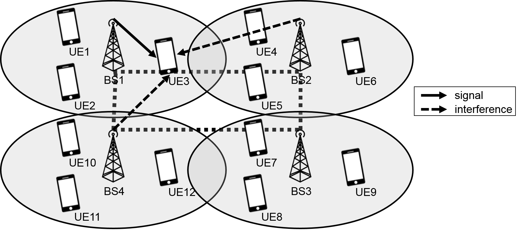 Figure 1
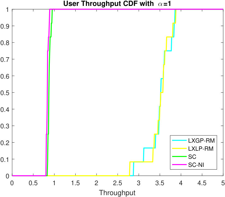 Figure 2
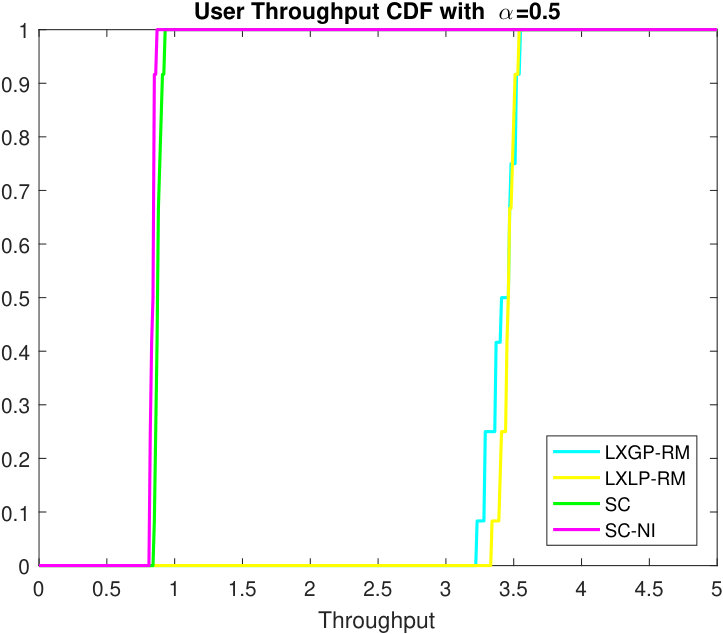 Figure 3
| Node | Before localization | After localization |
|---|---|---|
| 1 | , , , , , , , , to 2, 4 | , , to 4, , , to 2 |
| 2 | , , , , , , , , to 1, 3 | , , to 1, , , to 3 |
| 3 | , , , , , , , , to 2, 4 | , , to 2 |
| 4 | , , , , , , , , to 1, 3, 5 | , , to 1, 5 |
| 5 | , , , , , , , , to 4 | , , to 4 |
| Channels/Users | 0 | 1 | 2 | 3 | 4 | 5 |
|---|---|---|---|---|---|---|
| LXLP-RM Channels | 0.3447 | 0.6316 | 0.0237 | 0 | - | - |
| \hdashlineLXLP-RM Users | 0.3447 | 0.5395 | 0.1158 | 0 | 0 | 0 |
| LXLP-PL Channels | 0.3763 | 0.6105 | 0.0132 | 0 | - | - |
| \hdashlineLXLP-PL Users | 0.3763 | 0 | 0 | 0 | 0.0079 | 0.6158 |
| SC Channels | 0 | 0 | 0 | 1 | - | - |
| \hdashlineSC Users | 0 | 0 | 0 | 0 | 0 | 1 |
| Algorithm | LXGP-RM | LXLP-RM | LXLP-PL | SC |
|---|---|---|---|---|
| Utilities | ||||
| 89.61 | 89.73 | 86.98 | 19.62 | |
| 182.7 | 182.5 | 182.1 | 86.10 | |
| Iterations required | ||||
| 280.3 | 176.9 | 176.2 | 2 | |
| 273.6 | 216.9 | 142.9 | 2 | |
Peer Reviews
No public reviews on file for this paper yet. If you reviewed it on a platform where reviews are public (OpenReview, ICLR, NeurIPS, ICML), you can paste yours below so the community can read it here.
Videos
No videos yet. Explain this paper in a talk, walkthrough, or lecture? Add one.
\newsiamthm
factFact \newsiamthmexExample
\headersLocalization and Approximations for Distributed Non-convex OptimizationH. Kao and V. Subramanian
\externaldocumentex_supplement
Localization and Approximations for Distributed Non-convex Optimization
††thanks: Submitted to the editors on June 14, 2021.
Hsu Kao Electrical and Computer Engineering, University of Michigan, Ann Arbor, MI (). [email protected]
Vijay Subramanian Electrical and Computer Engineering, University of Michigan, Ann Arbor, MI (). [email protected]
Abstract
Distributed optimization has many applications, in communication networks, sensor networks, signal processing, machine learning, and artificial intelligence. Methods for distributed convex optimization are widely investigated, while those for non-convex objectives are not well understood. One of the first non-convex distributed optimization frameworks over an arbitrary interaction graph was proposed by Di Lorenzo and Scutari [IEEE Trans. on Signal and Information Processing over Network, 2 (2016), pp. 120-136], which iteratively applies a combination of local optimization with convex approximations and local averaging. We generalize the existing results in two ways. In the case when the decision variables are separable such that there is partial dependency in the objectives, we reduce the communication complexity of the algorithm so that nodes only keep and communicate local variables instead of the whole vector of variables. In addition, we relax the assumption that the objectives’ gradients are bounded and Lipschitz by means of successive proximal approximations. Having developed the methodology, we then discuss many ways to apply our algorithmic framework to resource allocation problems in multi-cellular networks, where the two generalizations are found useful and practical. Simulation results show the superiority of our resource allocation algorithms over naive single cell methods, and furthermore, our approximation framework lead to algorithms that are numerically more stable.
keywords:
Distributed optimization, non-convex optimization, localization, proximal approximation, resource allocation.
{AMS}
90C26, 90C90
1 Introduction
Distributed computation has received great attention in response to the overwhelming need in applications [30, 13]. In all of these applications there are multiple agents or devices with their own local data that want to perform a joint computational task that is either impractical or infeasible to be centralized. Reasons for this choice include high communication costs, availability of large amount of information, unavailability of centralized processing, or simply harnessing the efficiency of parallelization [30, 13]. Some specific examples are as follows: communication networks, e.g. scheduling and allocation in a multi-cell setting; sensor networks, e.g., remote parameter estimation with sensor data [30]; and statistical machine learning, with large datasets. In all of these cases the underlying computational task can be formulated as an optimization problem, with objective being utilities, loss functions, etc. [13]. Such motivations have lead to a burgeoning of the research in distributed optimization.
Distributed optimization methods with convex objective functions have been well investigated in the literature. Many proposed methods fall into the category of gradient or subgradient methods [26], which take gradient descent steps at each node and then average the results. Another class of methods utilize a dual-decomposition idea, like the Alternating Direction Method of Multipliers (ADMM) method [10]. In contrast, distributed non-convex optimization has received much less attention. One of the first provably convergent algorithms for non-convex objectives using a fully distributed scheme, called NEXT, over a network with arbitrary graphical structure was introduced in [24]. The main idea in [24] is to perform local optimization by finding surrogate convex functions based on the current iterate and utilizing successive convex approximations of the non-convex objective, and then enforcing consensus among the network so that a global objective can be solved in a distributed manner. Other papers on this topic assume much stronger conditions, such as existence of a central controller to align the outputs in each step [15], or even a complete graph network (interaction) structure [22]. Given this we will adopt the framework of NEXT [24] in our work. Here we consider the scenario where the network that specifies the communication structure is given; the reader is referred to [19] for how to decide the network structure actively, with minimizing the energy consumption for delay-constrained singular value decomposition computation as a motivating example.
There are some fundamental issues with NEXT [24] though, which we will address in our work. First, the algorithm requires each node to store and update the entire vector of decision variables, irrespective of the underlying dimension or structure; this is also an issue more broadly for most distributed optimization algorithms. In certain applications, the decision variables might be the ensemble of sets of control parameters at each node, which could be of a significant dimension themselves: e.g., multiple platoons of automated cars with a local controller for each team, or cellular base-stations each with many connected devices. Directly using NEXT would necessitate greatly increased storage at each node and also high-rate and low-latency communication between all nodes, which is impractical for a large network. In the illustrative examples above, the decision variables typically can be decomposed into blocks with a sparse interconnection between different blocks. Such a block structure could be used in reducing the storage and communication requirements. This, however, has not received much attention in the distributed optimization literature. The block coordinate descent method for centralized optimization is studied in [4], wherein gradient descent is effectively carried out one block at a time. When the objective is the sum of separable functions, convergence is shown for extensions of ADMM when the number of blocks is two [4], but this no longer holds when there are three blocks [11]. A distributed optimization scheme for variables with block structure is proposed in [14], but only the convex part of the objective is decomposable. An optimizatiton problem where the separable variables of agents are coupled through a convex social cost function is studied in [36], where the author uses a dual method to decouple the variables and leverage the separability; the goal is to show that the duality gap vanishes when the number of agents grows. In our work we will address this lacuna and present an algorithm that exploits the underlying block structure of the decision variables through a process which we call localization when the objective is the sum of separable non-convex functions. Our idea of localization is similar to [37], which exploit the sparsity of the constraints in convex feasibility problems (CFPs) to reduce the memory and communication needed. As we will explain in Section 4.3, not only is our framework more general, but it also works for non-convex problems.
A second issue with the approach in [24] is that the objective in many applications may not have the required smoothness. For example, the common assumption is of Lipschitz and bounded gradients as in [24], but this may not hold; we will demonstrate this explicitly with the motivating application. In centralized convex optimization, apart from subgradient methods, proximal methods are used for non-smooth functions [29]: e.g., a substitute is the Moreau envelope that is strongly convex and maintains the minimizer. We will develop a general scheme for continuous objective functions with non-Lipschitz unbounded gradients that takes any sequence of smooth approximations as input, such as the Moreau envelope.
Motivating Example
There is a trend for increased access-point deployment density coupled with the increasing usage of high-speed connections as well as fiber for backhaul [39, 2] in modern wireless networks. Hence, it is feasible to envisage high-rate and low-latency communications based coordination between neighboring base-sites to implement distributed optimization methods for resource allocation. Even this only allows communication of locally relevant decision variables, and rules out communicating network-wide decision variables, as would be the case if one used the algorithm in [24]. We will use the resource allocation problem, solved via the Network Utility Maximization framework [28] with some specific use cases described in [16, 17], as our motivating example. In the one-shot weighted sum-rate maximization problem derived from the decomposition of network utility across time instances in a time-varying channels environment, we have to jointly decide the power transmitted by base stations (BSs) at each channel (power control), as well as the resource blocks (RBs) a BS should transmit data to its users (scheduling); jointly this is termed resource allocation. This problem is hard because the objective is non-convex, and the constraints are knapsack-like constraints; the latter are usually solved by relaxing to real-valued variables and then rounding. We will follow the same approach, and concentrate on obtaining (locally) optimal solutions to the relaxed problem. While this problem for the single-cell is well characterized [16], the solution to even the multi-cell power control problem with interference impacts remains unresolved [12].
Given the difficulty of solving the multi-cell resource allocation problem, existing methods in the literature use heuristic approaches such as decomposition of the problem followed by greedy algorithms that lead to sub-optimal solutions [35], or make strong assumptions on the network interference graph [40]. Some algorithms are centralized [38], which is an impractical assumption in a realistic scenario. Prior work [33] also utilizes interference prices to solve the multi-cell power control problem, where each BS-user pair maximizes its own utility minus the sum of marginal “costs” to all other users with increase in its power. This literature only considers power control and not scheduling. Also, though having extensions in multi-channel settings, only one receiver is considered under each transmitter, and users need to sequentially broadcast their interference prices to ensure convergence in the multiple-input single-output case. In [31], a distributed power control and scheduling algorithm is proposed; -optimality is established for the grid network with a -hop interference model.
In this paper, we generalize the results in [24] by resolving the two issues mentioned earlier. For the first issue, we exploit the separability of the decision variables and the objectives’ partial dependencies to reduce the storage and communication needs. Although all components of the decision variable are entangled via each node’s objective, we show that each component can be maintained and optimized within a local network – this is different from directly applying NEXT to the setting, and its convergence is not obvious from [24]. Secondly, inspired by the proximal method, we use a series of functions with Lipschitz gradients to approximate the original objective, and significantly relax the smoothness assumptions made in [24]. We show that as long as the series of approximation functions approach the original function slowly enough, we are still guaranteed to obtain stationary solutions in many situations. While following the same steps as NEXT when the gradients are Lipschitz, our algorithm appears to have superior numerical stability over NEXT with non-Lipschitz gradients. We establish convergence for our algorithm with the proposed two generalizations under the condition of no unbounded gradients on the boundary. We then apply the results and algorithms to the multi-cell resource allocation problem in many different ways, which gives numerous algorithms with provable convergence to locally optimal solutions. Last but not least, we give a stochastic approximation interpretation of NEXT in Appendix D, where we provide an alternative proof of NEXT and discuss its relation to [6].
The rest of the paper is organized as follows. We describe the distributed optimization problem setup and the idea of NEXT in Section 2. Then we present our generalized algorithm with localization and proximal approximations in Section 3. In Section 4, we discuss the effect of localization, as well as address the practicability issues of our algorithm. We give examples where gradients are unbounded such that NEXT fails to converge to the correct solution while our algorithm does. We describe the application to the multi-cell resource allocation problem in Section 5. We discuss simulation results for the approximation functions and resource allocation application in Section 6, and conclude in Section 7.
2 Preliminaries
In this section, we give the system model of distributed non-convex optimization and assumptions. The bulk of the setup directly follows from [24]. Consider a network that consists of nodes. We aim to solve an optimization problem of the form
[TABLE]
where all ’s are smooth but can be non-convex, and is convex but may be non-smooth. The goal is to let these nodes cooperatively solve the problem in a distributed fashion. Therefore, each maintains a copy of the entire decision variable , referred to as . Then Eq. 1 is equivalent to solving the optimization problem
[TABLE]
at each subject to the constraint that all nodes agree on their optimal choices, i.e., we enforce
[TABLE]
In the context of distributed optimization, node only has the information of . It would require communication between the nodes to solve the problem in Eq. 2-Eq. 3.
Below are the standard assumptions on the objective functions and the constraint set.
**Assumption A
(A1)** The set is closed and convex;
(A2) is convex with bounded subgradient for all ;
(A3) is coercive, that is, ; based on this we can effectively assume that is compact;
(A4) ’s have bounded gradients, i.e. s.t. for all .
The set of nodes along with a set of undirected edges form a graph . This graph captures how communications take place – node and can only communicate if . is assumed to be connected to foster communication between the nodes; otherwise, the problem is generally unsolvable111All results can be trivially extended to directed time-varying graphs: see [24] for NEXT and the Appendix for our algorithm. For easy of presentation we adopt the above settings..
Our methods follow the solution scheme of NEXT. In the NEXT algorithm, each node performs a local convex optimization, and then some information will be exchanged in the network. At a high level, the first step is the “descent step” and the second is the “consensus step;” the two steps are iteratively applied to obtain the solution [24]. In the first step of time , the node solves a convex approximation of the whole objective function by convexizing its own objective function parametrized by the current iterate to be a strongly convex surrogate function , while linearizing the sum of other nodes’ objective functions . We assume the surrogate function satisfies the following assumption:
**Assumption F
(F1)** is convex;
(F2) for all ;
(F3) Either ’s are coercive for all and or is coercive.
The result established is convergence to the stationary solutions, whose definition is given as follows.
Definition 2.1**.**
*A point is a stationary solution of Problem Eq. 1 if a subgradient exists such that for all . *
3 Main Result
In this section, we introduce our two generalizations – localization and approximations of NEXT, which are the key contribution of this paper. We will first describe our settings for the generalizations, and then give the revised algorithm and the convergence theorem.
3.1 Localization Setting and Assumptions
Consider the setup where there are local dependency sets , and the local objective function of node , i.e. , only depends on a common variable and the local variables whenever . To be more specific, the decision variables can be split into parts where is an arbitrary positive integer. For all (which stands for ), define the local dependency set . Denote the sizes of as . We can think itself as the -th local dependency set and every may depend on . We adopt the convention that whenever appears in either superscript or subscript, it means or anything associated with the original network ; this includes . In the other direction, define the dependent part . Note that for all , contains . Also, when appears in the superscript of a variable, for example , it means the vector concatenated from all ’s such that , i.e. . Concrete examples of local dependency sets are provided in Section 4.1. Furthermore, we have the following assumptions:
**Assumption L
(L1)** Besides the fact that depends on only if for , also only depends on ;
(L2) The set is separable, i.e. it is the direct product of convex sets in proper subspaces such that for all if and only if ;
(L3) The local network is connected for all 222We add nodes to get connectedness if it does not hold. More on this in Section 4.2, we already assume the connectedness of in Section 2;
(L4) For all there is a matrix associated with – each entry is non-zero if and only if there is a corresponding edge in , and all non-zero entries must be greater than or equal to some fixed . Equivalently, for all rows and all columns , we have and . In addition, is doubly-stochastic after deleting these zero rows and columns. does not contain zero row or column, and corresponds to the defined in NEXT.
Note that ’s do not have to be disjoint and form a partition of . Having for some is allowed. Without loss of generality we can assume they form a covering of ; i.e., . When there exists a part on which all ’s and depend, then is itself; otherwise, nodes outside the union do not have any cross-dependence with all the rest and can be optimized themselves.
3.2 Proximal Approximations Setting and Assumptions
In contrast to the common setting in the optimization literature, we consider a scenario where is not Lipschitz continuous for some . Our idea to relax this Lipschitz assumption is to use a sequence of functions whose gradients are Lipschitz continuous to approximate . This is commonly known as the proximal approximation method in the literature of convex optimization, except that our objective is now non-convex.
To be more specific, we want to find a series of functions such that is globally Lipschitz continuous with constant and that as we have pointwise, or even better – uniformly. Then at iteration we can use the well-behaved instead of . We will see that as long as the schedule of satisfies certain conditions, we can still have convergence to optimality.
The following assumption is the key feature of that our algorithm needs for convergence to optimality.
Assumption N:
(N1) is globally Lipschitz continuous with constant ;
(N2) uniformly, and pointwise.
We will also need a surrogate function of , denoted as . These surrogate functions should satisfy Assumption F´ similar to Assumption F given as follows.
**Assumption F´
(F1´)** is uniformly strongly convex with constant ;
(F2´) for all ;
(F4´) is uniformly Lipschitz continuous with constant .
As [24] does not have approximation functions, they assume Assumption F´ for the surrogate function of , i.e. , with fixed and . Here our assumptions are more general than NEXT in that we do not require the strong convexity of and the Lipschitz continuity of . In particular, we can have and as long as the schedules of and satisfies certain conditions. We do have an additional Assumption F3. However, that assumption is implicitly implied if ’s are strongly convex; thus, we do not lose any generality from [24]. Also for simplicity, we assume is a non-decreasing sequence. We denote .
3.3 Localized Proximal Inexact NEXT and Main Convergence Theorem
Our localized proximal inexact version of NEXT, which requires less storage and communication, and allows unbounded non-Lipschitz objective gradients, is presented in Algorithm 1. All operations that contain index , i.e. Line 5, 6, 7, 9, 10, and 11, are performed for all . Also, except Line 5, the operations have a superscript , and are performed for all . In Line 5,
[TABLE]
with and . Note that Line 6 along with Line 5 means that one solves the optimization problem in Eq. 4 with accuracy . Also denote . The output of the algorithm is the concatenation of , where .
NEXT is a special case of Algorithm 1. First, NEXT would either be the case where for all , or the equivalent case where consists of one part only. In the NEXT algorithm, node keeps the whole , and communicates the whole as well with all of its neighbors; the same also applies to the variables and . On the contrary, under our localization setting, node turns out only has to maintain (also and ) in Algorithm 1; moreover, it only communicates (also ) with its neighbor . This could mean substantial savings for memory and communication, especially when the dependency structure is sparse. Section 4.1 provides an example that explicitly specifies the storage and communication needed before and after localization. Secondly, NEXT would be when , , and for all and . Algorithm 1 also accommodates a bigger class of objective functions and supports a more flexible choice of the schedules of and .
Remark**.**
*The insight of the variables and can be found in [24]. In short, node needs the information of at the current iterate when linearizing others’ objectives. For this purpose, node tracks the average of gradients using , keeps its neighbors updated, and obtains , an approximation of , by subtracting its own gradient from . In our localized algorithm, only nodes in participate in the decision of and the tracking of and , which requires some subtle treatment. *
Remark**.**
*Note that Algorithm 1 is not the result of the direct application of NEXT in the localization setting given in Section 3.1. Suppose is such that and under the connectedness assumption. Different from NEXT, node no longer keeps the gradient trace in Algorithm 1, nor does the variable appear in the objective of the local optimization. The fact that convergence can still be obtained with Algorithm 1 is not obvious from [24]. *
The following theorem generalizes the convergence to stationary solutions result of NEXT when gradients are bounded, specifying restrictions on the schedules of , . When gradients are unbounded, stricter constraints are needed.
Theorem 3.1**.**
For all , let be the sequences generated by Algorithm 1, be their averages, and be the ensemble of averages. Let , , , , , and .
- (a)
Suppose Assumptions A, F, L, N, and F´ hold333Note that Assumption N1 requires where with given as Eq. 6. For any other choices of other than the double Moreau envelope function [21], Assumption N1 requires for any such that is non-Lipschitz continuous.. Also, is such that , , . Then (1) all sequences asymptotically agree, i.e., ; (2) is bounded, and its limit points are stationary solutions of the original problem. 2. (b)
If we do not assume Assumption A4, but we have , , , , and . Then we still have results (1) and first part of (2). When the limit points lie in the interior of , or is bounded on those limit points, they will be stationary solutions. 3. (c)
Continuing (b), if a limit point lies on the boundary of and , then the definition of stationary solution does not apply, and could be a local minimum, or a point that is not a local minimum.
Proof 3.2**.**
*See Appendix B. *
Remark**.**
*Note that the conditions in (a) imply . In (b) we apply the stricter as well as other constraints. *
We can see that although all parts of the variable are coupled through all the objectives ’s, the decision on is actually dictated by the nodes in . We give a class of approximation functions that satisfies Assumption N, namely the Lasry-Lions envelope or double envelope [21], in Section 4.4. Note that the convergence of Algorithm 1 only requires the Lipschitz constants of follow certain schedules, but can be any sequence of functions that approaches in the limit, and does not need to be double envelope. We will give many examples of such sequences in Section 4.6 and Section 5.4. Also, an example of the schedules of the the parameters , , , and that satisfies the related conditions in Theorem 3.1 (a) and (b) using -series is given in Section 4.5. We will discuss the unbounded gradient issue in full detail in Section 4.6, study different examples there, and show the numerical stability of our algorithm for these examples in Section 6.1.
4 Discussions
In this section, we discuss some details of our proposed algorithm. Two localization examples that compare the effect of localization are given in Section 4.1. We comment on how to exploit localization when Assumption L3 is violated in Section 4.2. Comparison to the localization algorithm proposed by Hu et al. in [37] is given in Section 4.3. Section 4.4 and Section 4.5 summarize the property of double envelope that we will use and provide the -series example for the parameters , respectively.
4.1 Examples of Localization
In this subsection we give a few examples to illustrate the concept and effectiveness of localization.
{ex}
Consider the communication graph given in Fig. 1 (a). In this example we consider the most common situation, where the dependency is directly given by the communication graph. Specifically, every node has a corresponding variable part in the whole variable tuple . Moreover, the objective at node only depends on its own variable and its neighbors’ variables . In other words, the local dependency set corresponding to is equal to . is assumed to be [math]. This situation also arises in the resource allocation application we discuss in Section 5.
For this communication graph, this situation will be the following. The variable can be split into five parts, and we have ( only depends on , , and ), , , , and . The local dependency sets for this example are given in Fig. 1 (b). Before localization, node 1 needs to store all of to and communicates this information to its neighbors . In contrast, after localization node 1 only keeps , , and , and exchanges some of this information with . In addition, node 1 does not maintain the information of , , or , , either. Before localization, NEXT performs
[TABLE]
in the local optimization step at node 5, while after localization Algorithm 1 performs the following
[TABLE]
The first terms of the two operations are actually the same. Indeed, since only depends on and , we can definitely choose a surrogate function that only depends on the local storage of and . The difference is node 5 does not have to store, say , and optimize based on . The variable is asymptotically tracking . Our localization result says that since node 5 does not have any preference on , it only follows others’ decision of through . Hence, it is unnecessary for node 5 to maintain and – it can just take other nodes’ decision at the end, even through and are coupled through, say . This saves nodes from unnecessary memory storage and communication in the presence of sparse dependency structure, which is crucial when the network is large.
{ex}
We consider the same communication network but a different dependency structure: , , , , and . There are three local dependency sets in this example as shown in Fig. 1 (c). The variable parts that are stored at each node and the communication required to other node for each part are given in Table 1. Naturally, before localization every node keeps all parts and communicates them with all of its neighbors. On the contrary, the storage and communication required are greatly reduced after localization. Notice that even though node 3 is directly linked with node 4, they do not communicate as there is no common part they both depend on.
4.2 Relaxing Assumption L3
Our requirement of connectedness of is not a strong assumption. If any is not connected, we can always “add” nodes as “relays” into the local dependency set. For example, consider Section 4.1 with revised to be a constant and revised as . Then is not connected. We can add node 3 into by making where the dependency is actually trivial. Node 3 can thus relay the information of for node 2 and 4. Alternatively, node 1 can also do the relay job. Hence, we assume without loss of generality that the nodes have been added by some algorithm that might depends on network structure and communication requirements so that every is connected.
4.3 Comparison to Hu et al.
In [37], a similar idea of localization for convex feasibility problems (CFPs) is proposed, where they also exploit the sparsity of the constraints to reduce the storage and communication required. Our framework is different from theirs in two aspects. First, in their framework each node owns a part of the variable tuple , whose corresponding “dependency network graph” must be a subgraph of ’s local graph where is ’s neighbors in the communication graph . On the other hand, in our framework each part of the variable tuple does not have specific relation with the nodes and the local dependency set is only required to be a connected component in , which is more general in the sense that their framework is a sub-case of ours. Second, their dependency is built in the constraint sets, while ours is based on objective function’s dependency. This difference arises from the nature of CFPs and optimization problems. Namely, we focus on solving the optimal solution for optimization problems while they aim to find the solution lying in the intersection of a batch of sets. Although one would be able to solve convex optimization with CFP algorithms [9], it is still unclear whether this could be generalized to the case of non-convex optimization.
4.4 An Example of Approximation Functions Satisfying Assumption N
The Lasry-Lions envelope or double envelope [21][32] is a class of approximation functions that serves this purpose. We use this to illustrate the feasibility of our approach but also point out that any such sequence of functions satisfying the assumptions and conditions can be used instead.
Definition 4.1**.**
The double envelope, or Lasry-Lions envelope [21][32], of a function is defined by
[TABLE]
*where . *
Fact 1**.**
*If is lower bounded, then is Lipschitz continuous with constant . *
Fact 2**.**
* pointwise as . If further we have being uniformly continuous, then uniformly as . Furthermore, pointwise as . *
Proof 4.2**.**
*See [3]. *
Now it is clear that if we define
[TABLE]
then we have being globally Lipschitz continuous with constant . Since is coercive (Assumption A3), we can restrict our attention to some compact set in , where is uniformly continuous. Then over this set, we will have uniformly as well.
4.5 An Example of Sequences Satisfying the Conditions Using -series
Examples of the tuples satisfying the conditions of Theorem 3.1 exist with all schedules in -series form. Assume , , , and for some positive constants , , , and . Then the constraints on the parameters are
[TABLE]
A possible tuple satisfying the above equations is . If the ’s are Lipschitz continuous and then constant for all , then and the above requirements degenerate to and as in [24].
4.6 Examples of Objectives with Unbounded Gradients
When it comes to non-Lipschitz gradients, a first example might be functions with unbounded gradients, but this need not be the only case; for example, on . Its derivative is , which is obviously bounded on but actually not Lipschitz continuous on . Though convergence is not established for this case in [24], NEXT still works well numerically in these kind of simple examples. Next we turn to more challenging examples with unbounded gradients.
{ex}
[Interior local optimum] Consider in a triangle network, with , , and , where . There is no . The unique stationary solution is as . The derivatives for the node objectives are , , and . Obviously the derivatives are unbounded at for and , and this example is thus not covered in the theory developed in [24].
On the other hand, we can simply choose the following approximation functions: and with derivatives being and . We can choose throughout. One may check that and . The conditions in Theorem 3.1 (b) are checked in the following.
- •
series conditions: suppose we choose and , since , if we further choose then it is evident that all conditions are satisfied.
- •
: we actually have for all and hence .
- •
: the maximum differences of derivatives for node 2 and 3 always occur at , and for the choice . The condition holds because .
- •
: notice that for our choices of and the summed term equals and thus is summable.
- •
: notice for all .
As we have finite in , by Theorem 3.1 it is guaranteed that our algorithm converges to the unique stationary solution , which is also a global minimum in this example. Note that this minimum lies in the interior of .
{ex}
[Boundary local optimum] Consider a one node network, and the objective function is on the region inside the unit circle , so that the graph of , namely , is the upper half of the unit sphere lifted in the direction of positive -axis. For the upper half of the unit sphere, the set of global minima is the unit circle; now that we tilt the sphere, the unique global minimum is . There is no stationary solution inside the unit circle. Since the gradient
[TABLE]
is unbounded on the unit circle, the definition of stationary solution fails there. This example again clearly lies outside the theory of [24].
We consider the approximation function . Its gradient can also be obtained by changing the ’s in the denominators of the original gradient to . We have .
- •
series conditions: choose and , and .
- •
: notice that monotonically. Since the largest decreasing of always happen on the unit circle, is simply evaluated on the unit circle, which is .
- •
: roughly for the choice of . The condition is true because .
- •
: the term is decaying in the rate of , which is summable.
- •
: this one is obvious as we only have one node.
Our method will not converge to any point in ; otherwise, by part (b) of Theorem 3.1 we know it must be a stationary solution, but there is no stationary solution inside the unit circle. Thus, our method will converge to some point in ; since is infinite on the unit circle, this falls into the case of Theorem 3.1 (c), and the point is not guaranteed to be a local minimum. Even so, we find in Section 6.1 that for a wide range of initialization of , our algorithm can converge to while NEXT does not. Unfortunately, since the objective is symmetric with respect to -axis and the unique global maximum is , if we start with any point to the right of the maximum on the -axis, the process will inevitably approach in the limit.
We will see in Section 6.1 that NEXT fails numerically in the above examples while our method works much better.
5 Application to Resource Allocation
We now describe how to apply our algorithmic framework to wireless resource allocation, and along way also describe how the two issues that motivated our generalizations arise.
5.1 Problem Formulation
We consider an OFDMA wireless cellular network, where a set of base stations (BSs) transmit downlink data to users through the set of channels or resource blocks (RBs) . For a BS , denotes the set of users associated with it, which is an input that’s fixed. The transmitted power of BS in channel is denoted by , and the maximum total sum power transmitted by BS is limited to . The allocation variable of BS to user in channel is denoted by , with gain : means transmits to in the RB , and otherwise. For all users, we also introduce a scheduling weight, for user . Finally, is the variance of the independent zero mean additive white Gaussian noise (AWGN) for all BSs. We assume that BS only possesses the information of . In other words, BS can only compute the weighted-sum rate of the users associated with itself (knowing the powers of the other base-sites). This is a reasonable assumption, as each user equipment (UE) reports its measured channel gains to the BS it is associated with, whereas all the channel gains of UEs served by other BSs is unknown.
When the BS transmits a non-zero power in channel , it interferes with all the other transmissions in channel . However, owing to propagation-based loss, the powers of nearby BSs will dominate the whole interference term. Hence, with the definition that is the neighboring BSs of BS , we can neglect all the interference from to . This is a modeling assumption that is reasonably accurate in practice, and will be in force henceforth. For ease of exposition we assume that neighbor relation is mutual, i.e. if and only if . In terms of the interference graph, where nodes are BSs and edges only exist between BSs that interfere with each other, we reduce a complete graph to an undirected and connected one. Our work can be trivially extended to the directed case assuming that strong connectivity holds.
We consider a one-shot weighted sum-rate maximization problem, subject to the allocation limit constraint, the power limit constraint, non-negative power constraint, and the fact that is either [math] or ; we will justify the weighted sum-rate maximization problem in the next section. To make the overall constraint set convex, we relax the integer constraints on as in [16, 17]. In future work we will study appropriate integer rounding schemes.
The joint power control and scheduling problem (P1) is then formalized as:
[TABLE]
where and are the signal and interference for user in channel . We use to refer to the collection of the variables ; also, can be viewed in a similar way, where . This is a shorthand for easy referencing.
As we will solve the problem in a distributed manner, we let each BS maintain the decision variables . Denote the copy of at BS by for all . The idea is to perform the optimization at each BS, and then enforce consensuses of the decision variables among all BSs, transforming (P1) into (P2) given in the following:
[TABLE]
where and . The set of constraints includes all the constraints in Eq. 7 now with and the second and fourth constraints hold for all copies at , and an additional constraint that the consensus is reached .
We can split the term in the objective to two parts and , and then modify the former to be as in [16, 17], which is jointly strictly concave in and . We define the modified function to be 0 when so that it is continuous. Then (P2) becomes the following:
[TABLE]
subject to the same set of constraints as in Eq. 8. Note that (P2) and (P3) are the same if ’s are restricted to be integers, that is, .
We will now reiterate the two issues we identified earlier with existing distributed optimization approaches but in the specific context of Eq. 9. If we take the approach in [24], then every BS would need to keep a copy of all the decision variables, both and , and perform consensus on them and also any relevant gradient terms. This is simply impractical and forces the localization idea. We also note that Eq. 9 contains functions of the form x\log\big{(}a+(p+p^{\prime})/x\big{)}-x\log(a+p^{\prime}) that are smooth but where the gradients are not Lipschitz; in particular has some terms of its gradient becoming infinite when . These functions clearly fall outside the framework of [24], and force approaches like our proximal approximations scheme. In the following, we apply the developed distributed optimization framework to the problem in Eq. 7-Eq. 9. In the problem, the set of BSs in the cellular network corresponds to in the framework, a BS corresponds to a node , and the set of edges in the framework is the one-tier interference graph here. There are many different ways to apply our framework to the resource allocation, which we discuss in detail next.
5.2 Direct Method
In this method, we directly let be the weighted sum-rate of BS : , and . In the first version of this method, every BS keeps the powers of all BSs as decision variables, that is, we have for all . But instead of keeping ’s as decision variables at BS for all if we exactly follow NEXT, we allow every BS only keeps its own , which we denote as for short. As we see from Section 3.3, this suffices because BS dictates the decision of .
If we reconsider the problem from the perspective of our localization framework Section 3.1, there are local dependency sets. There are local dependency sets for all which correspond to the variables , and local dependency sets for all which correspond to the variables . In the first version of the direct method, referred to as the Localized X Globalized P-diRect Method (LXGP-RM) algorithm, only follows the localization framework, is still globalized in the sense that every BS keeps a copy of the whole variable.
We only present algorithm in words here, for the pseudo code see Appendix B. The algorithm basically proceeds as Algorithm 1 with the common variable and local variables (and without approximation functions since objectives have Lipschitz gradients). At BS we use to track and to track , which correspond to and in Algorithm 1. In each iteration, we let , and BS performs the minimization of
[TABLE]
with respect to the variables and , and , , and being the current iterate of the variables. The surrogate function is chosen as
[TABLE]
where and are functions of , but is just a function of . The quadratic term in LABEL:11 is to maintain the strict convexity of the surrogate. Finally, we have a universal doubly stochastic matrix to average and for them to reach consensus. We remark that with the objective in Eq. 10 only having up to quadratic terms and our constraints being linear, the minimization can be solved efficiently using quadratic programming (QP) with coefficient matrices of the quadratic term being positive-semidefinite [20].
The second version of the direct method, termed as the Localized X Localized P-diRect Method (LXLP-RM) algorithm, makes better use of our localization idea as opposed LXGP-RM so that for all we now only maintain the variables for in BS , as the BSs in dictate the decision of ; the variables still follow the localization framework just as before in LXGP-RM. The main change from LXGP-RM is that the index set of the variable tuple is now replaced by , as BS does not keep the variable for any more. As a result, the steps regarding the weighted sum for reaching consensus need to be modified. We introduced the matrix for each BS . The matrix concerns with the weighting of the local dependency set regarding the variable , that is, where if the whole network is . Its -th row and -th column should be zero if and only if or . After deleting all these zero rows and columns, it would become a doubly-stochastic matrix, as described in Assumption L4.
The second version of the direct method still follows the framework of Algorithm 1, with local variables and no common variable. Now at BS we use to track , and to track , where . Also, the surrogate is minorly changed so that now the quadratic term of only sums over instead of .
We finally remark that one can also consider a GXGP-RM algorithm (basically NEXT from [24]) where copies of both the power and allocation variables are maintained at each node, or even a GXLP-RM algorithm where localization is performed only for the power variables. Note that only the fully localized scheme, i.e. LXLP-RM, will be scalable in practice. However, we will evaluate its performance relative to the other schemes.
5.3 Decomposed Method
In (P3), there is a part of the objective that is concave (or convex after taking minus sign), and the optimization of this part should be easy. The algorithm might run faster if we properly exploit this fact. To achieve this goal, let us assume that the channel gains ’s are known to all BSs. Then we could apply the framework in Section III by letting and G=-\sum_{b,i,k}w_{i}x_{bik}\log\big{(}\sigma^{2}+\tfrac{\Gamma_{bik}+\bar{\Gamma}_{bik}}{x_{bik}}\big{)}.
As is in general a function of not only but also for all and we need to optimize at every BS, this method does not allow any localization. In other words, the tuple consisting of all decision variables is the common variable in Algorithm 1 itself, and there is no local dependency set besides itself. At BS we need to maintain as well as . Note that with the derivatives of being Lipschitz continuous and no localization, this method is a direct application of [24].
The algorithm, which we call the Globalized X Globalized P-deComposed Method (GXGP-CM), is also largely the same as LXGP-RM, except that now we have to optimize as well, and we need to maintain and update . The algorithm and the surrogate function also need minor revisions (see Appendix B).
5.4 Partially Linearized Method
While the decomposed method enjoys the benefit of using the intrinsic convex part in the objective, it is impractical since it requires every BS knows all channel gains. We could instead put the convex part in as well, and take advantage of it by not linearizing it when forming the surrogate function. Specifically, we let where and . Then we can choose the surrogate function as , where has exactly the same form as in LABEL:11 (for LXGP case), i.e., linearized with the current iterate plus the quadratic terms.
With not being Lipschitz continuous, we have to apply the approximation functions detailed in Section 3.2 to guarantee convergence. We may choose where
[TABLE]
One can easily show that is Lipschitz continuous with constant the reciprocal of . We can then choose a schedule of according to Theorem 3.1 and Section 4.5. We refer to this method as the Partially Linearized method (PL) algorithm, which could be LXLP or any of the other combinations. Note that we do not have the guarantee of convergence to stationary solution in this case because the objective function has unbounded gradient on the boundary.
5.5 Consensus Scheme
Let be the BS network we are considering, and let be the degree of BS . The choice of must meet the following two criteria to conform to Assumption L4: (1) it must be doubly-stochastic; (2) is non-zero if and only if . We denote the set of ’s that satisfy these criteria as , which is a subset in . We choose as follows
[TABLE]
where . It is easy to verify that this choice of is row-stochastic. Since is symmetric, it is then also column-stochastic. By definition of , we will have . By construction, if .
In LXLP-RM algorithm we need a for every BS . Let . Then we choose as described above but treat as .
With symmetric weights , [23] suggests that the best convergence speed is obtained with the solution of
[TABLE]
For symmetric graphs, the optimized result is when and otherwise, which is exactly our choice.
6 Simulation Results
In Section 6.1 we compare the performance of Algorithm 1 with NEXT of the examples with unbounded gradients on either interior point or boundary point described in Section 4.6. In Section 6.2 we compare our algorithms with single-cell scheduling and resource allocation method.
6.1 Approximation Functions
Fig. 2 depicts how the local decision variables in Section 4.6 change for NEXT and Algorithm 1 within iterations. We start with initial value of . We choose the following parameters: (independent of and ), , ,
[TABLE]
and the surrogate functions are chosen to be direct linearization plus the quadratic regularization term (see LABEL:11 for an example of such kind of choices). In Fig. 2 (a) we can see that NEXT oscillates and is not numerically stable for this example. Whenever the iterates go near the global minimum at , they jump to values far away. This is because the gradients and are infinite at the point, even though is zero there. The trackings of to and to are in the fast time-scale (see Appendix D) and actually happen quite fast, as can be seen in the figure. However, a slight mismatch between and is sufficient to cause very large , which is supposed to be very small when , driving ’s to the boundary. If two of them jump to and one of them to , then in the next few iterations they jump up; if two jump to and one to , they jump down.
We cannot ensure that NEXT is not converging when theoretically, but we observe it is still oscillating when is as large as . In contrast, Algorithm 1 essentially converges to the global minimum within iterations in Fig. 2 (b). In Fig. 2 (c), we show the case when , where we have everything satisfied except – one can check there will be an additional term. From the figure we see that not only it exhibits oscillating behavior, but it seems to converge to a wrong point other than .
The converging behaviors of NEXT and Algorithm 1 for Section 4.6 are shown in Fig. 3 for two different initializations. The parameters are , , and . The surrogate function is again direct linearization plus quadratic regularizer. The 2-D iterates for both algorithms are plotted from red to blue, with NEXT being circle dots and Algorithm 1 being square dots. In Fig. 3 (a), we start with , and both algorithms are executed for iterations (the dots are down sampled though). We see that while our algorithm is converging to the global minimum at , NEXT is “converging” to some point near the boundary. Due to the unbounded gradient near the boundary, the term in is completely dominated by the rest , which directs the iterate only to descend in the radial direction. Again we cannot ensure NEXT does not converge to if we run it forever; however, it does not visit the region after iterations. By slowly changing the objective, we are able to escape this dominance and obtain the correct solution.
In (b) we start from , which is to the right of the global maximum , for iterations, and both algorithms are converging to . Since we start on the -axis and the gradients always direct to , without any perturbation there is no way to escape -axis for all gradient-descent-like methods. Section 4.6 falls into the case (c) in Theorem 3.1, where the algorithm is converging to some point in the boundary and is not bounded. The definition of stationary solution does not apply, and NEXT fails to converge to global minimum for both and , while Algorithm 1 succeeds for but also fails for .
6.2 The Resource Allocation Application
We adopt the framework of the network utility maximization problem as in [16, 17] where we maximize
[TABLE]
where is given by
[TABLE]
is the average throughput of user up to time , is the fairness parameter, and is a QoS weight. The gradient-based scheduling approach [27] leads to solving the optimization problem given below at each time instance
[TABLE]
This is exactly the one-shot optimization problem we consider in Eq. 7, where is the weight of user , is the rate of user given by the Shannon capacity, and is the capacity region dependent on current channel state and constrains the choice of as the constraints set in Eq. 7.
Now consider problem Eq. 7. A naive solution would be disregarding the interference and solving the resource allocation and scheduling for each cell separately. The optimization for a single-cell is well solved in literature, e.g. in [16]. Specifically, neglecting the interference, for a BS we can solve
[TABLE]
subject to the constraints. This is a convex problem, and can be solved with existing methods in convex optimization. We call this method the Single-Cell No-Iteration (SC-NI) algorithm.
A refinement of the SC-NI algorithm is to update the interference terms after first optimization for each cell. We then optimize for each cell again while treating the powers of neighboring BSs as constants, and then repeat until convergence. We call this the Single-Cell (SC) algorithm.
We adopt the 19 cell wrap-around model from [18] as the network scenario used in our simulations. Furthermore, each UE associates with exactly one BS and each BS has five UEs associated with it. Suppose a UE is served by a BS. Then there is a signal link between the UE and the BS, while all the neighbors of the BS cause interferences to the UE. The time horizon is chosen to be . The channel gains are directly generated by Rayleigh distribution, with parameter for associated BS-UE pair, and for interference, instead of choosing random locations for the UEs and calculating the path loss. The channel gains are assumed to be independent among all links in a scheduling instance and also across all scheduling instances. We use identical QoS weights (). Other parameters include: , , , , and . For simplicity we treat all scheduling terms as real numbers and use the local optimal results to compute utilities. In future work we will include integer rounding procedures in the simulations. The entire process is simulated only one time, as multiple time slots already brought in the averaging effect.
Fig. 4 depicts the CDFs of user throughput of algorithms LXGP-RM, LXLP-RM, LXLP-PL, and SC for (maximum total throughput) and , respectively. When , we can observe that the RM and PL methods stochastically dominate the SC algorithm, and this is also nearly the case when . In fact, the RM and PL methods yield a roughly 4-fold average throughput gain over SC method. This is not surprising, as we simulate a rich interference environment, and the new methods can coordinate the scheduled UEs and transmission powers of nearby BSs, while the SC method does not. The RM methods show similar performance as we use the same termination criteria. They are a little bit different from the PL method possibly due to optimizing different objective functions (only equivalent before integer relaxation).
Fig. 5 illustrates the power and SINR distributions of the same four algorithms for . The proposed three new methods choose one of three values for the power: the maximum, half of the maximum or zero. This corresponds to assigning either one, two or no blocks; the two blocks can be assigned to one UE or two. On the contrary, the SC methods schedule all three blocks and UEs with the power to each block around . At each time instance the three new methods give up serving some subcarriers and users in exchange of boosting the SINR of the scheduled UEs on the chosen blocks. On the other hand, the SC method tries to serve everyone, and ends up with lower power and increased interference. The details of the scheduling decisions are in Table 2.
Table 3 compares the performance of the four algorithms with and . The three coordination-based methods outperform the SC method significantly in this problem instance. The LXGP method always requires more iterations to converge than the fully-localized methods like the LXLP family. When , LXLP-PL converges much faster than RM methods.
7 Conclusion
In this paper, we generalized existing distributed non-convex optimization methods in two directions. First, we reduced the algorithm storage and communication complexity by exploiting a decomposable structure of the problem, and obtained a localized algorithm. Second, we relaxed the requirement of Lipschitz continuous gradients with a series of slowly-changing approximations. We then applied the developed algorithmic framework in different ways to generate distributed algorithms for the multi-cell resource allocation problem; the flexibility of implementing our framework is also a contribution. We compared these algorithms with the single-cell algorithm via simulation and showed the potential gains of using the distributed optimization methods developed.
Appendix A Generalizations to time-varying graphs
In this appendix we provide the less strict assumptions to accommodate the case where the underlying graph is time-varying and directed. The proof of our result is based on this more general setting. But the purpose of these assumptions remains the same – a distribution on the set of nodes will go to the uniform distribution exponentially fast with repeated application of the matrix, which is captured in Lemma B.2.
At each time slot , the set of nodes along with a set of time-variant directed edges , form an directed graph . Node can only send message to node in time slot if .
**Assumption L´
(L3´)** is -strongly connected for all , where , i.e. is strongly connected for all ;
(L4´) For all there is a matrix associated with – each entry is non-zero if and only if there is a corresponding edge in , and all positive entries must be greater than or equal to some fixed . As before, is doubly-stochastic after deleting the zero rows and columns whose indices are not in .
Appendix B Proof of the Main Result
In this appendix we prove Theorem 3.1. We start with an intuitive description of the roadmap of the entire proof in the following. Our proof follows the main structure of [24]. The convergence of NEXT basically consists of two parts – at the faster time scale the “consensus convergence” of local variable iterates and local gradient iterates to the average iterate and (the average gradient evaluated at the average iterate), respectively, and on the slower time scale the fixed point iterations of (defined in Eq. 45) which we call “path convergence” – for details of this viewpoint and connection to two time-scale stochastic approximation see Appendix D. It is shown in [24] that the fixed points of coincide with the stationary solutions. The goal is thus to prove the iterates converge to the fixed points of and the iterates of all nodes asymptotically agree. Our contributions are introducing partial dependency structure with a localization scheme and in addition successively approximating the possibly non-Lipschitz gradient objective functions. The latter significantly increases the proof hardness as the gradients of the objective functions may now be unbounded.
The core idea of NEXT as in most primal algorithms, is in performing the following steps iteratively.
- •
The local optimization step for each node is to find the value of at its iterate . This maps the iterate to the optimum of an approximated strongly convex version of the overall objective function , which involves using a strongly convex surrogate for ’s own objective function, and a linearized approximation of others objective functions. This step is similar to doing gradient descent in a much more efficient way by taking advantage of the surrogates, and corresponds to the “path convergence” mentioned above.
- •
The consensus step is where every node communicates its iterate to its neighbors and also takes an average of its neighbors’ iterates. We refer to the ’s asymptotically agreeing on their average as the “-consensus convergence.”
To make the algorithm more practical and fully decentralized, the original Inexact NEXT [24] and our Localized Proximal Inexact NEXT add multiple layers of approximations.
- (1)
We mentioned that the node linearize other nodes’ gradients with . However, node only has the information of . It hence keeps a variable that tracks the average gradient so that node can approximate by with the knowledge of and as in Algorithm 1. The convergence of to the average gradient is then the “-consensus convergence.” The convergence is also achieved through a gossip-type consensus scheme similar to that used for . 2. (2)
With the approximation scheme using the variable, the fixed point iteration we actually use in Algorithm 1 for the local optimization step is defined in (4), which is similar to but using as the linearization constant. This makes the algorithm viable in practice in a fully decentralized scenario. To compare the behaviors of and , we construct a new “averaging system” assuming that the ’s already converge to ; this includes , the average gradient evaluated at , and , the local optimization map where computed from is used as the linearization constant. Note that this “averaging system” is constructed purely for analysis purposes. 3. (3)
We use a series of functions to approximate so that the local optimization map with ideal linearization is , and with the -approximation in contrast to just in NEXT. This is the approximation we add in addition to what was done in Inexact NEXT [24]. 4. (4)
The inexactness of the algorithm chooses within range of , which leads to another source of approximation. Because of the function approximation we use with the relaxed constraints on the schedules of and , the difference between and can potentially become increasingly larger if the error propagates, which also increases the proof hardness in contrast to the case of Inexact NEXT where the difference is bounded.
The proof of Theorem 3.1 consists of six parts. The theorem basically makes two claims: the nodes’ iterates asymptotically agree, and they converge to one of the optima. The former will be the side product as we aim to prove the latter. In the first part of the proof, we first summarize the list of notations that will be used in the proof in Section B.1, and then describe a few results and one key proposition in Section B.2. Proposition B.1 as the variant of Proposition 5 in [24] shows Lipschitz properties of . Lemma B.2 and 3 describe the main machinery we use to show the “-consensus convergence” and “-consensus convergence,” that is, the geometric convergence of the product of doubly stochastic matrices to the all one matrix. The results Lemma E.1, Lemma E.2, Lemma E.3, and Technical Assumption T are technical lemmas regarding series or summations that arise in the analysis. The key proposition is Proposition B.3, which constitutes the core components of the proof.
We prove Proposition B.3 (a) in the second part Section B.3, which says the difference between and cannot grow beyond a certain rate, and the tools used are the definition of minimization (4), the strong convexity of , and the -consensus convergence. The difference is decomposed into and , where the former is bounded by by definition, and the latter is bounded by using a mathematical induction argument.
Part (b) of Proposition B.3 establishes asymptotic consensus on among nodes as the third part of the proof Section B.4. This part involves exploiting Lemma B.2, Lemma E.1, 3, Part (a) of Proposition B.3, and series convergence. The generalization to multiple local dependency sets is also taken care of in Part (a) and (b) of Proposition B.3 using simple inequalities regarding multi-dimensional spaces.
In the fourth part contained in Section B.5, Part (c) of Proposition B.3 is proved, which shows that the locally-optimized result using the “ approximation” converges to the locally-optimized result with ideal linearization evaluated at . In addition to applying the definitions of the maps, it is intuitive that the “-consensus convergence” in the “averaging system” and hence Lemma B.2 play a crucial role in the proof; Part (a) of Proposition B.3 and Technical Assumption T which comes from Lemma E.3 and the conditions of Theorem 3.1 are also used.
We prove Part (d) of Proposition B.3 in the fifth part Section B.6. Part (d) claims the actual locally-optimized result in the algorithm converges to the locally-optimized result using the “ approximation” . The underlying reason of the convergence is the “-consensus convergence.” Several previous results are all used in this proof, including all of Parts (a), (b), and (c), Lemma E.1, Lemma E.3, and Technical Assumption T.
Section B.7 then combines Parts (a), (c), and (d), convexity of , and Lemma E.2 to show that converges to . With going to [math], is no longer a function but a correspondence; variational analysis is thus introduced to deal with the minimizers of correspondences in the first case of Section B.7. Finally, we deal with unbounded gradient interior point in the second case of Section B.7, using convexity and series convergence. Generalization to study the case of an unbounded gradient boundary point is left as an open question.
Comparing to the proof of NEXT, the generalization to multiple local dependency set is not a technically hard one; it requires some simple inequalities as shown in part (a) and (b) of Proposition B.3. For the second generalization, we replace what was Lipschitz constant and strongly convex constant by series and , which now could grow to infinity and decrease to zero, respectively. This does significantly increase the hardness of the proof. The conditions in Theorem 3.1, the Technical Assumption T stated below, and Lemma E.3 are made such that all the series now with and still converge. The unbounded gradient issue and the correspondence nature of also make our scheme much trickier to analyze in comparison to NEXT.
B.1 Notations
We define a set of notations to proceed with the proof. All notation is defined for all , , and , whenever applicable.
Original variables
- •
: the concatenation of part decision variables from all nodes in with padded zero for nodes not in ; we also use to refer to non-padded zero version , i.e. the vector containing only when is in , when the context is clear; the notation , which denotes the vector concatenated from all the vectors of the form where the index is in the set , will be used throughout this Appendix
- •
: the concatenation of part of , which tracks the average (among nodes) gradients of from the nodes in in the algorithm
- •
: the concatenation of ground truth gradient, with ; adding is unnecessary as the gradient would be zero for those nodes not depending on
- •
: the gradient difference, with ()
- •
: see Line 11 of Algorithm 1
- •
: see Line 5 of Algorithm 1 and Eq. 4
Average variables
- •
: average of decision variable
- •
: average of gradient tracking variable
- •
: average of ground truth gradient
- •
: average of gradient difference
Tracking system using average variables
- •
- •
: the concatenation of ground truth gradient evaluated at average decision variable
- •
: the gradient difference evaluated at average decision variable, with
- •
: tracking of average gradient evaluated at average decision variable, with ; concatenating for makes
- •
- •
: optimized result evaluated at average decision variable and average tracking system
- •
: average of ground truth gradient evaluated at average decision variable
Doubly stochastic matrices
- •
- •
- •
- •
, where , and is the identity matrix
- •
, where is the identity matrix with dimension
B.2 Key Propositions
The next proposition is a variant of Proposition 5 in [24].
Proposition B.1**.**
Let be the concatenation of for all in . Define the mapping by
[TABLE]
and the mapping by , that is, preserving everything in the subspace unchanged while mapping with in the subspace. Then, under Assumptions A, F, and N, the mapping has the following properties:
- (a)
* and ,*
[TABLE]
where . Here we use and interchangeably as they are the same thing. 2. (b)
* is Lipschitz continuous, i.e. for 444Note that this holds for as well because the elements in the subspace just cancel each other out.. *
The only thing we do is to substitute in [24] as . Although the equations are written in localization form, it does not really change anything here.
Lemma B.2**.**
Define . Then under Assumption L´(doubly stochasticity and lower bounded entries for edges),
[TABLE]
*for some and . *
Strictly speaking the above is for the , which is the matrix used for the averaging of the entire network, in Assumption L´. For where , the Lemma also holds after we delete the zero rows/columns. In this case the product converges to where the is of the proper dimension. From now on we will take as the largest geometric convergence factor among all , .
Before proving Theorem 3.1, we will first prove the following proposition.
Proposition B.3**.**
Let and , be the sequences generated by Algorithm 1, in the settings of the Theorem 3.1. Then the following holds:
- (a)
For all , . 2. (b)
, , . 3. (c)
, . 4. (d)
, .
We will use the following assumption frequently when proving Proposition B.3. These are the exact technical inequalities we use in the proof, while all of them are implicitly implied by the conditions of Theorem 3.1 as we will show below.
**Technical Assumption T
(T1)** ;
(T2) ;
(T3) for all and ;
(T4) ;
(T5) ;
(T6) for all and .
Proof B.4**.**
(T1)*: it should be evident from the conditions of Theorem 3.1 that none of the parameters could be growing or decaying at an exponential rate. We are considering the setting where and are going to zero while is going to infinity. The condition implies that if either is growing exponentially or is decaying exponentially, then must also be decaying exponentially. But then would never be possible.
(T2): recall the conditions of Theorem 3.1 imply , then apply the first part of Lemma E.3.
(T3): from and the first part of Lemma E.3.
(T4): again the parameters are not growing at an exponential rate.
(T5): from and the second part of Lemma E.3.
(T6): from and the second part of Lemma E.3. *
B.3 Proof of Proposition B.3 (a)
Consider a local dependency set and any node . By the definition of defined in the minimization of Eq. 4, we have
[TABLE]
From the Line 11 of Algorithm 1 and (F2´), we have
[TABLE]
Substitute this result into Eq. 20 and rearrange the terms to get
[TABLE]
We have omitted all the time indices in LABEL:30 since all the variables have the same time index .
Suppose that is bounded by for all . Then LABEL:30 is of the form
[TABLE]
which implies that all ’s are bounded by 555Note that refers to and is in as well if the part exists. Therefore, the second term can be put into the summation in the first term.. This is due to the following argument: if are non-negative and , then ; otherwise, W.O.L.G. we can assume and hence , then the following holds
[TABLE]
which is a contradiction. Thus, with Eq. 23, we get
[TABLE]
where is some constant independent of and . This proves the claim. It only remains to show that is actually bounded by .
We use mathematical induction to finish the proof. The statement is that
[TABLE]
holds for all . We have already shown that the latter implies the former. The base case is obvious as we initialize to be , which is assumed to be Lipschitz continuous. For the induction step, we assume the statement is true for and proved the latter part holds for .
By the definition of , we have
[TABLE]
where
[TABLE]
To reach the last line we utilize the triangle inequality and the Lipschitz continuity of . For the first term,
[TABLE]
Using the induction hypothesis of , we obtain
[TABLE]
Therefore, we finally obtain
[TABLE]
using the induction hypothesis of and the fact that also goes to zero when implied by the condition of Theorem 3.1.
B.4 Proof of Proposition B.3 (b)
We only prove the case for to save the ubiquitous subscript of . The proof of the claims for general is exactly the same with appropriate substitutions of by .
- (i)
[TABLE]
Notice that with 3 (d) and (e), the difference of and which is can be expressed as a linear combination of and . We can thus expand iteratively as follows:
[TABLE]
where the last equation resulted from 3 (b). From Proposition B.3 (a) we know
[TABLE]
for some constants and . Consequently, we get
[TABLE]
by first utilizing triangle inequality, and then using Eq. 29, Lemma B.2, and finally Lemma E.1 (a). Remark that implies , which we use in Eq. 30 as the condition of Lemma E.1 (a). 2. (ii)
[TABLE]
The bound for the last term comes from Lemma E.1 (b). 3. (iii)
[TABLE]
The bound for the first term is natural. The double summation is bounded due to the second equality Lemma E.1 (b) with being . The condition of Theorem 3.1 guarantees that . The inequality of the triple summation follows from
[TABLE]
where the last inequality is due to the first equality of Lemma E.1 (b). Again, the convergence of is implied by the convergence of .
B.5 Proof of Proposition B.3 (c)
We exploit the optimality of and (F1´) and (A2) to get
[TABLE]
and the optimality of (for the mapping of ) leads to
[TABLE]
is an all zero vector in the subspace . It should be clear that refers to the component of in the subspace . Then
[TABLE]
From LABEL:40,
[TABLE]
Up until now, the context is clear enough to allow us to drop all time index. Again, we only focus on the case of ; that is, proving goes to zero. We calculate
[TABLE]
and
[TABLE]
Similar to LABEL:31-2 we have
[TABLE]
Similar to the technique as in Eq. 28 to (30), by combining Eq. 34, Eq. 35, plus Lemma B.2, and then LABEL:41, we have
[TABLE]
In the last equation, we also have and implied by the conditions of Theorem 3.1. For the second part of the claim, we can equivalently prove
[TABLE]
This is true because
[TABLE]
All the terms are finite because of the following. The first term is due to (T4) – after multiplying a going-to-zero , the term remains to be bounded. The second term is due to (T5). The third term is in the condition of Theorem 3.1. The fourth term is due to (T6). The last term is also in the condition of Theorem 3.1.
B.6 Proof of Proposition B.3 (d)
Recall we have and , where
[TABLE]
These along with (F1´) and (A2) lead to the following:
[TABLE]
and
[TABLE]
As we did in LABEL:40,
[TABLE]
Hence,
[TABLE]
Since is not larger than , LABEL:45 implies the former goes to zero as goes to infinity if we can show all terms in the RHS do so. The first term does go to zero as we showed in part (b) (combining Eq. 30, Lemma E.1 (a), and the fact that ). The following shows this property holds for the remaining two terms as well. As always we omit all time index from above as the context is clear enough.
We have
(40)
and
[TABLE]
For the terms of the form to converge to zero, refer to Eq. 30 and Assumption T1 and T2. In the second line, from Eq. 34, Eq. 35, and Section B.5 we know that can be represented as a sum of ’s; using the same method can also be represented as a sum of ’s, which we omit here. In the last inequality one can alternatively use Eq. 27 to bound and , which is simpler and sufficient for our purposes.
For the second part of the claim,
[TABLE]
For the first term, use Eq. 30, (T4), and (T5). Second term is finite due to (T4) with additional . The terms in the forth line are just like the first term. The terms in the fifth line converge by the condition of Theorem 3.1. The terms in the second line are of the type , from Eq. 30 and (T4) one can show that converges, hence the convergence of the terms by applying second part of Lemma E.3. The terms in the third line converge because of (T6).
B.7 Proof of Theorem 3.1
Denote . By descent Lemma,
[TABLE]
By the convexity of (A2),
[TABLE]
Then using Proposition B.1 (a) and the fact that has bounded subgradients,
[TABLE]
where stands for the expression . Combining Section B.7, LABEL:50 and (N1) with Cauchy-Schwarz inequality as well as triangle inequality, we get
[TABLE]
From the triangle inequality, Proposition B.3 (a) and 3 (e),
[TABLE]
Substitute these expression back into (LABEL:51) and rearrange the terms to get
[TABLE]
We now exploit Lemma E.2 with , and
[TABLE]
Since is coercive ((A3)), ; on the other hand, from Proposition B.3 (c), (d), and the assumption of the Theorem, . Thus, by Lemma E.2 converges to a finite value and converges as well, which means
[TABLE]
This in turn implies
[TABLE]
At this point the localization is no longer an issue, and we will use the generalized definition of so that we have for all .
Since is bounded following from the convergence of , there exists a limit point of the set. We assume . If this is not the case, then one can find a subsequence indexed by such that as . We consider a partition of three cases: (1) bounded gradient (), (2) unbounded gradient and interior point (), and (3) unbounded gradient and boundary point ().
(1) bounded gradient: Recall the map defined in Proposition B.1
[TABLE]
This map is converging to the following map
[TABLE]
which might be multi-valued since we do not require to be strongly convex. The latter map is well-defined everywhere only with bounded gradient. Otherwise could be infinite; moreover, when and , it is not possible to achieve , being defined everywhere and being convex simultaneously. Thus, the analysis for this case does not work for the other two cases.
Now consider the two maps evaluated at and respectively, , the minimizer of , and , the set of minimizers of . We have the following two properties.
- •
is eventually level-bounded, i.e. , is bounded. Refer to [32], p. 8, p. 109, and p. 123 for the definitions of the notations. This is ensured by Assumption F3, i.e. either is coercive or is coercive.
- •
, i.e. epi-converges to . See [32], p. 241 for the definition. This is due to and being continuous and , then by [32] Theorem 7.2, p. 241 we have .
By [32] Theorem 7.33, p. 266, with these two properties, we then have
[TABLE]
In [24] Proposition 5(b) says that the fixed point of is also the stationary solution of the original optimization problem, which is proved in [14] Proposition 8(b). Things change slightly here as the minimizer of may not be unique. However, in the proof they did not exploit any strong convexity property. Hence, we still have being a stationary solution.
(2) unbounded gradient and interior point: Effectively we want to show
[TABLE]
but we can no longer argue anything with . Only for the following we will write instead of for simplicity. From the optimality condition of , we have that for all ,
[TABLE]
where is just . The terms in the second bracket are bounded as follows
[TABLE]
where the second inequality is due to the Lipschitz continuities of and . Since we assume in the condition and get , it must be that . Hence, with the conditions of and , taking in Eq. 47 yields exactly Eq. 46. It is evident that must be a point such that , because if not so is an interior point and there must exist one descent direction.
(3) unbounded gradient and boundary point: We can consider two subcases.
- •
: we can use the same argument in case (2) to show that is a stationary solution. If we have , we can also use the same argument in case (1) confined to a small neighborhood of .
- •
: the definition of stationary solution fails here and we can only turn to the definition of local minimum. However, both NEXT and our algorithm can numerically converge to a point which is not a local minimum.
Appendix C Pseudo Code of the Algorithms
In this appendix we give the complete pseudo code of algorithms in Section 5 for reader’s reference. All ’s represent for compression.
C.1 LXGP-RM
The LXGP-RM algorithm is given as follows:
In the algorithm, is the collection of the variables , and so are the other quantities , , etc. The collection of variables can be viewed as a matrix, or a vector of dimensions. is a matrix (or vector) consisting of all 1’s. denotes the element-wise product, also known as Hadamard product or Schur product.
C.2 LXLP-RM
Using the same notations as in LXGP-RM, the LXLP-RM algorithm is given as follows:
In line 10, the notation stands for being updated as for all , and so do line 11 and 12. In line 12, means the degree of , i.e. . If considering to be a matrix, then consists of rows; each row has elements, and every element in the -th row is .
C.3 GXGP-CM
the GXGP-CM algorithm is given as follows:
Appendix D A Stochastic Approximation Viewpoint
In this appendix, we review NEXT from the viewpoint of stochastic approximation. We provide an alternative proof of Theorem 4 in [24] using results from stochastic approximation in Section D.1. As we will see, NEXT can be seen as a two time-scale process, with the faster tracking the total gradient, the slower tracking the fixed point iteration of , and a repeated projection onto the consensus plane. From this viewpoint and the fact that the local optimization in Eq. 4 (in NEXT version, see Equation (8), [24]) can be solved by the projected gradient descent method described in Section D.2, we can interleave each “descent” as another time-scale of the algorithm. We relate the result with another distributed non-convex optimization method proposed in [6].
D.1 Alternative Proof of NEXT
Substituting the definitions of and into Inexact NEXT (Algorithm 2, [24]), we can rewrite each iteration of the algorithm in two steps:
[TABLE]
where , and is given by (8) in [24] with substituted by using (S.3) (c) of Algorithm 1 in [24]. By letting , Eq. 48 can be rewritten as
[TABLE]
where . It is evident that . As a result, Eq. 49 and Eq. 50 together form a two time-scale stochastic approximation algorithm [7], where or is on a faster, natural time-scale with constant step sizes, and goes on a slower, algorithmic time-scale with shrinking step sizes.
To analyze this process, we first begin with the fact that the fast variable or views the slow variable as quasi-static, i.e. we can see as constant in Eq. 50. Denote as the ensemble of ’s, i.e. , as the ensemble of ’s, and also , , etc. Then the iterate of will asymptotically track the following ordinary differential equation (ODE)
[TABLE]
where is the identity matrix, denotes the dimension of ’s, and means the Kronecker product. Then Eq. 51 would become
[TABLE]
Lemma D.1**.**
*We have . *
Proof D.2**.**
We have
[TABLE]
*where is the all one vector and . The second equality follows from the two matrices being multiplication commutative, third from , and fourth from the fact that . *
We see that indeed goes to the unique global asymptotically stable equilibrium, where every component of , i.e. ’s, equals to the average of the gradients as desired.
Next, from the perspective of the slow variable , the fast variable already reaches its equilibrium . That is to say, in Eq. 49 can be seen as , which is exactly , making Eq. 49 become
[TABLE]
As stated in [25], this recursive relation is again a two time-scale stochastic approximation in disguise, with fast averaging and slow learning processes. In fact, the averaging process is also on natural time-scale as . From [25] we know that the iterates of will reach consensus , while each of its component tracks the ODE
[TABLE]
as is the unique stationary distribution resulted from .
Note that with ’s being Lipschitz continuous ([24], Prop. 5a), this ODE is well-posed. We assume the differentiability of for now to avoid dealing with trickier non-differentiable Lyapunov function here. We consider the whole objective itself as the Lyapunov function . Then
[TABLE]
for some positive constant . The first inequality is established similarly as [24], Prop. 5b. By Lasalle’s invariance principle, the iterates converge to the set of equilibria ([8], p. 57 and p. 118), which is the set of stationary solutions of the original optimization problem ([24], Prop. 2).
We note that the conditions for applying [7] and [25] are either established in [24] or implied by the assumptions of Theorem 4 in [24]. Specifically, the boundedness of follows from the recursive relation Eq. 49 and Proposition 9 (a) in [24], , , and are just assumed in Theorem 4 in [24]. Note that we do not need as there is no noise in the recursion of . Also, we have deterministic convergence rather than almost sure convergence, since instead of being martingale differences, our noise term is actually deterministically bounded.
D.2 A Remark on Using One-Step Gradient Descent
Solving the local optimization in Equation (8) in [24] may be costly. Instead, from the stochastic approximation viewpoint, we can solve it iteratively as well using a time-scale faster than . Once again assume that is continuously differentiable to avoid working with subgradients. The optimization problem in Equation (8) in [24] belongs to the class of constrained convex optimization problems, and can be solved by projected gradient descent:
[TABLE]
where is some time-scale faster than and is the Euclidean projection onto the set
[TABLE]
Consider using the natural time-scale . The idea of stochastic approximation is essentially blending Eq. 57 into the original algorithm [34]. Namely, at instead of running Eq. 57 infinitely many times to exactly solve (8) in [24], we only run one step gradient descent of Eq. 57 from :
[TABLE]
and then use instead of in (S.2) (a) of Algorithm 1 in [24]. As converges, so does the coupling process of Eq. 57.
From the previous subsection we know that from the perspective of the slow variable , can be seen as , and thus as . Combining this, Eq. 58, and Algorithm 2 in [24] yield
[TABLE]
Note that Eq. 59 contains two projections. It is simple gradient descent followed by a projection to the consensus plane similar to Example 3 in [25], and then a further projection onto . Similar to Section D.1, the iterates of will reach consensus , while each of its component tracks the ODE
[TABLE]
called the projected gradient flow. From Proposition 5 of [6] (also [34], p. 10), works as a Lyapunov function for the set of its stationary solutions, then by Theorem 2 of [6] (also [34], Proposition 9 and Remark 10) the iterates converge almost surely to the set of stationary solutions666Again, “almost surely” is unnecessary here, since our noise is deterministically bounded.777If in general we consider , a Lyapunov function may not exist, and we are only guaranteed convergence to a “nonempty compact connected internally chain transitive invariant set” in [25]. A detailed tutorial covering the difference of these sets can be found in [5].888Coerciveness of is required to apply the LaSalle invariance principle. Without it, has to be analytic to make the set of local minima and the set of Lyapunov stable points of the gradient flow equal to each other [1]..
In Eq. 59, the matrix only needs to be column stochastic instead of doubly stochastic. There exists some distribution to which converges, and the ODE will be minimizing . It immediately follows that with doubly stochastic (which induces ), we can reduce in Eq. 59 to and still minimizing , implying that we can simply let the gradient of each node spread through the gossip and do not have to track and anymore. This is exactly what is done in [6] (with ).
The two papers [24] and [6] have their own strengths. The method in [6] can solve the whole problem using less computation power due to the high cost of local optimization, while NEXT not only allows non-differentiable but also achieves the optimal within fewer iterations. This is useful in delay sensitive applications with abundant computing resource.
Appendix E Technical Lemmas
We put some technical lemmas used in the proof in this appendix. Some of them are from [24].
Fact 3**.**
For all we have the following.
- (a)
, where we also have
[TABLE]
We use the equality in showing the above equation. 2. (b)
. 3. (c)
* where and are all arbitrary in .* 4. (d)
* where . This simply follows from Lines 7 and 9 of Algorithm 1.* 5. (e)
. This follows from applying (c) to (d).
Lemma E.1**.**
Let , and let and be two positive scalar sequences. Then
- (a)
If , then . 2. (b)
If further we have and , then and .
Lemma E.2**.**
*Let , , and be three sequences of numbers such that for all . If for all and , then either or converges to a finite value and . *
Lemma E.3**.**
*Let , and let and be two positive scalar sequences such that , , and . If further there exist and such that for all , then . Moreover, if is summable, then so is . *
Proof E.4**.**
The proof of the first part of the claim is straightforward.
[TABLE]
*The second term goes to zero by the condition. Note that the meaning of basically says cannot decay to zero faster than at an exponential rate. Thus, would imply that as well. For the second part of the claim, just sum Eq. 61 over . *
The reference list from the paper itself. Each links out to its DOI / PubMed record.
- 1[1] P.-A. Absil and K. Kurdyka , On the stable equilibrium points of gradient systems , Systems and Control Letters, 55 (2006), pp. 573–577.
- 2[2] M. Alleven , 5g, lte-a to drive long-term growth in backhaul market: Ihs . Available at http://www.fiercewireless.com/tech/5g-lte-a-to-drive-long-term-growth-backhaul-market-ihs , 2016.
- 3[3] H. Attouch and D. Azé , Approximation and regularization of arbitrary functions in hilbert spaces by the lasry-lions method , Annales de l’IHP Analyse non linéaire., 10 (1993), pp. 289–312.
- 4[4] A. Beck and L. Tetruashvili , On the convergence of block coordinate descent type methods , SIAM Journal on Optimization, 23 (2013), pp. 2037–2060.
- 5[5] M. Benaïm, J. Hofbauer, and S. Sorin , Stochastic approximations and differential inclusions , SIAM Journal on Control and Optimization, 44 (2005), pp. 328–348.
- 6[6] P. Bianchi and J. Jakubowicz , Convergence of a multi-agent projected stochastic gradient algorithm for non-convex optimization , IEEE Transactions on Automatic Control, 58 (2013), pp. 391–405.
- 7[7] V. S. Borkar , Stochastic approximation with two time scales , Systems & Control Letters, 29 (1997), pp. 291–294.
- 8[8] V. S. Borkar , Stochastic approximation: A dynamical systems viewpoint , Hindustan Book Agency, and Cambridge University Press, New Delhi, India, and Cambridge, UK, 2008.