Hypergeometric First Integrals of the Duffing and van der Pol Oscillators
Tomasz Stachowiak

TL;DR
This paper demonstrates the existence of hypergeometric first integrals for the Duffing and van der Pol oscillators, revealing new non-analytic integrals expressed via hypergeometric functions and providing a general criterion for such phenomena.
Contribution
It introduces hypergeometric first integrals for these oscillators and formulates a criterion for their existence in general dynamical systems.
Findings
Existence of Liouvillian first integrals expressed through hypergeometric functions.
These integrals are neither analytic nor algebraic.
A general criterion for hypergeometric integrals in dynamical systems.
Abstract
The autonomous Duffing oscillator, and its van der Pol modification, are known to admit time-dependent first integrals for specific values of parameters. This corresponds to the existence of Darboux polynomials, and in fact more can be shown: that there exist Liouvillian first integrals which do not depend on time. They can be expressed in terms of the Gauss and Kummer hypergeometric functions, and are neither analytic, algebraic nor meromorphic. A criterion for this to happen in a general dynamical system is formulated as well.
Click any figure to enlarge with its caption.
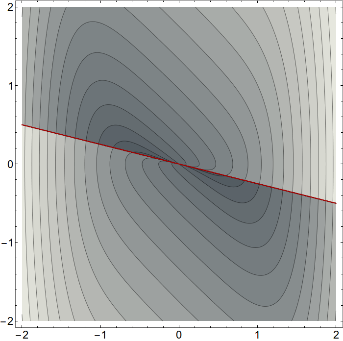 Figure 1
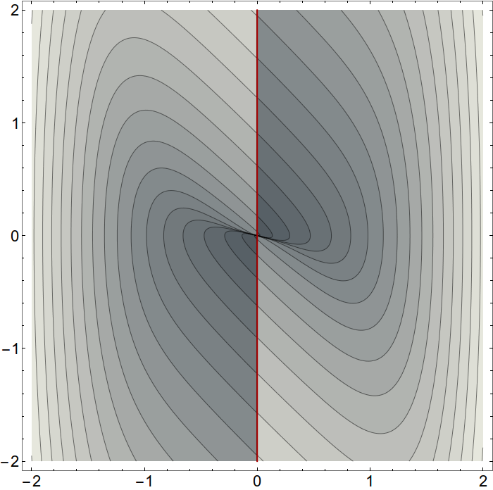 Figure 1
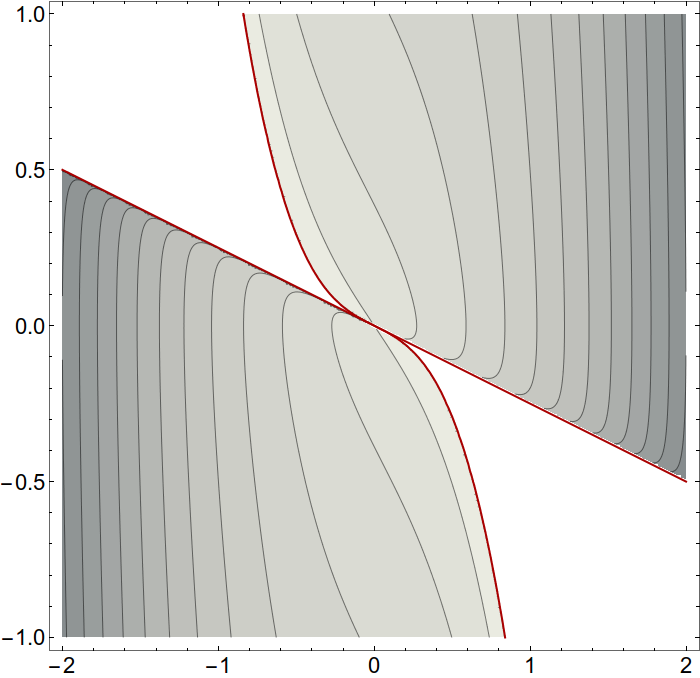 Figure 2
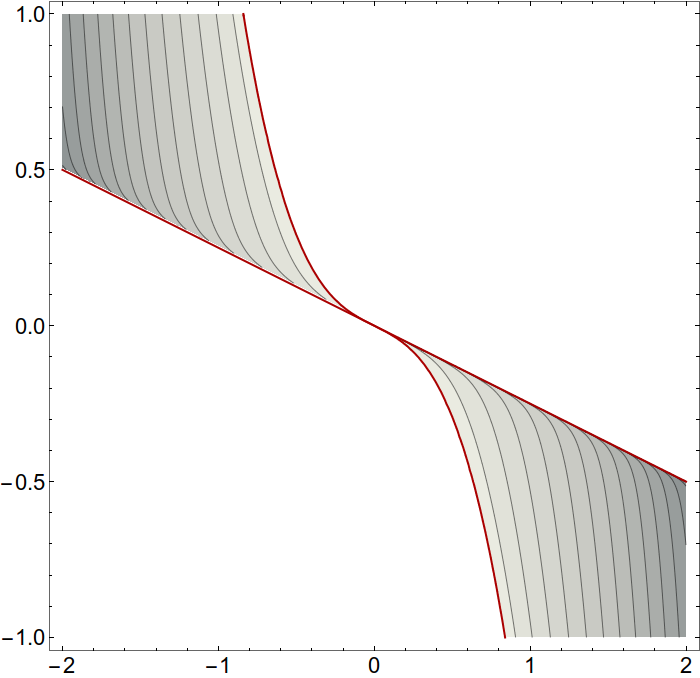 Figure 2
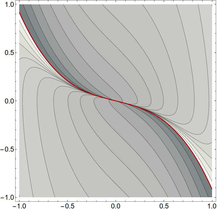 Figure 3
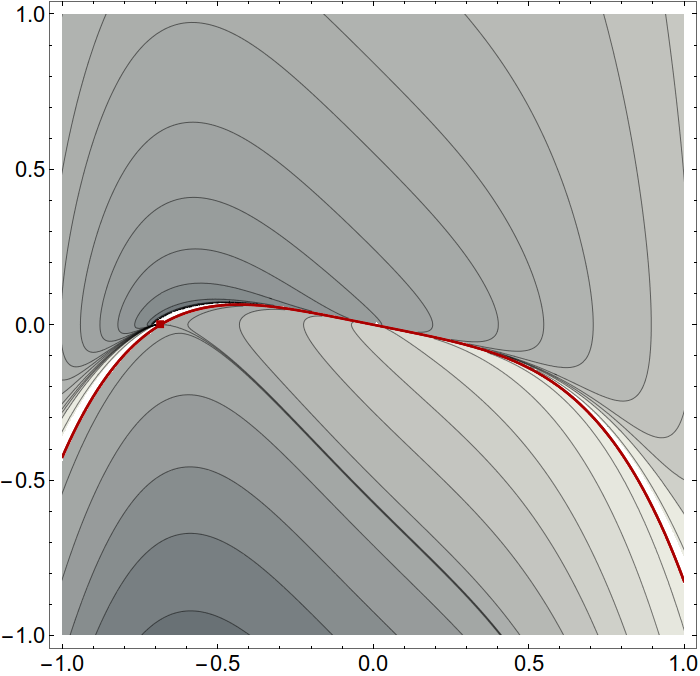 Figure 3
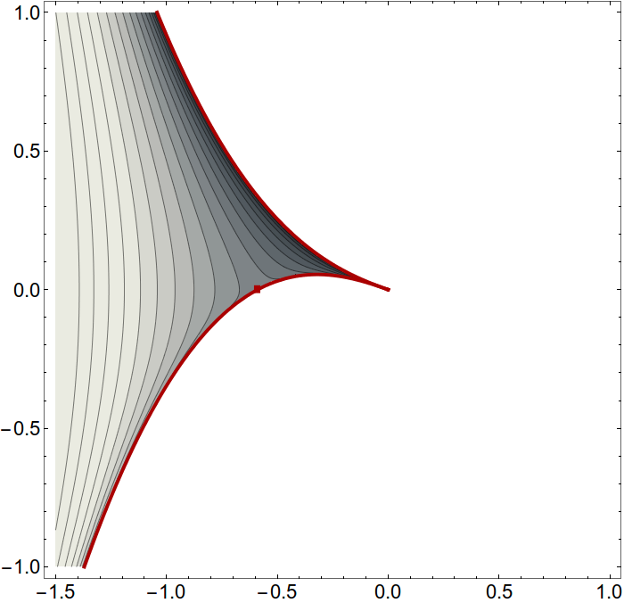 Figure 9
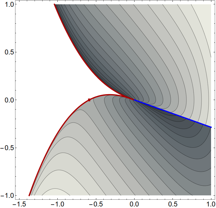 Figure 9
Peer Reviews
No public reviews on file for this paper yet. If you reviewed it on a platform where reviews are public (OpenReview, ICLR, NeurIPS, ICML), you can paste yours below so the community can read it here.
Videos
No videos yet. Explain this paper in a talk, walkthrough, or lecture? Add one.
Hypergeometric First Integrals of the Duffing and van der Pol Oscillators
Tomasz [email protected]
Department of Applied Mathematics and Physics,
Graduate School of Informatics, Kyoto University,
606-8501 Kyoto, Japan
Abstract
The autonomous Duffing oscillator, and its van der Pol modification, are known to admit time-dependent first integrals for specific values of parameters. This corresponds to the existence of Darboux polynomials, and in fact more can be shown: that there exist Liouvillian first integrals which do not depend on time. They can be expressed in terms of the Gauss and Kummer hypergeometric functions, and are neither analytic, algebraic nor meromorphic. A criterion for this to happen in a general dynamical system is formulated as well.
1
The Duffing and the van der Pol oscillators are among the simplest (at least in form) dynamical systems, present in biology [1, 2], nano-electronics and mechanics [3] as well as many subfields of physics [4, 5] (see the last one for a more comprehensive list of references). The systems’ integrability, or solvability, is still an active topic with only partial results available [6, 7, 8] and the aim of the present article is to use them as examples of how non-analytic Liouvillian first integrals can arise in polynomial differential equations. This is the content of Lemma 1 in Section 2 and its generalization in Section 5.
The force-free form of the basic Duffing oscillator is
[TABLE]
or, more generally,
[TABLE]
With a suitable rescaling of and the time, and can be made equal to 1, so the only essential parameters will be and . Although the case of immediate interest is that of integer , the extension to real is straightforward if is replaced by .
For the specific value of , explicit solutions of (1) in terms of Jacobian elliptic functions were found in [6]. The authors note that the equation admits a transformation
[TABLE]
which turns the equation into a solvable one
[TABLE]
It can be regarded as Hamiltonian with
[TABLE]
which is then conserved, but upon going back to and , the first integral defined by becomes time dependent:
[TABLE]
A generalization of the above approach, which utilizes transformations of the form (3), was formulated in [7], and gives a more constructive method of finding first integrals.
As the solutions are explicitly available, this time dependence of does not seem to be a practical problem – one could argue that a first integral can be obtained (at least locally) by elimination of time between the solutions, but that is seldom practically computable. Thus, the question emerges of whether a “proper” time-independent first integral exists. The goal of this investigation is to show that this is indeed the case for the general unforced Duffing oscillator, and partly so for the Duffing-van der Pol oscillator. What is more, the existence of such an integral can be ascertained without the a priori knowledge of the solutions.
The first main result of the present letter is the following
Theorem 1**.**
If the frequency of the Duffing oscillator (2) with general nonlinear term of degree satisfies
[TABLE]
then the equation has a Liouvillian first integral. When is odd, in the half-planes separated by the integral is given by
[TABLE]
where and ; alternatively, in the half-planes separated by it is
[TABLE]
with and as above. Each is real when its argument is less than 1.
When is even, so that defines a real invariant curve , the above expressions remain valid if is taken to the right of , and to its left with .
The second equation of interest is the Duffing-van der Pol oscillator, which exhibits the same type of time-dependent first integrals. The equation is
[TABLE]
and it was shown in [8] to admit a whole parametric family of time-dependent integrals. The required condition is that and , and the conserved quantity is
[TABLE]
Similarly to the previous system, this quantity can be used to obtain a time independent first integral, leading to the second result:
Theorem 2**.**
If the parameters of the Duffing-van der Pol oscillator (10) with general nonlinear term of degree satisfy
[TABLE]
then the equation has a Liouvillian first integral given by
[TABLE]
which is real when ; or alternatively by
[TABLE]
which is real when . Additionally, the singularities of the hypergeometric function correspond to the invariant sets and .
The above system can be further generalized to
[TABLE]
which was analyzed with the Prelle-Singer procedure in [9], and with the Lie symmetry method in [10]. It differs from the first two in that the specific structure of its invariant sets makes the hypergeometric first integral confluent:
Theorem 3**.**
If the parameters of the generalized Duffing-van der Pol oscillator (15) satisfy
[TABLE]
then the equation has a Liouvillian first integral given by
[TABLE]
where . The above integral is real, and its only singularity corresponds to the invariant curve .
The appearance of hypergeometric functions is quite remarkable – it shows how restrictive the notion of analytic, meromorphic or algebraic integrability can be. Although various parametric forms of solutions of polynomial dynamical systems can be given in terms of hypergeometric functions [11], this seems to be the first example of a natural (i.e. not artificially contrived) system with first integrals of such form. This is the price we have to pay for the transition from relatively simple, but time-dependent, integrals to time-independent ones, which permit us to call an autonomous system integrable in the standard sense.
A starting point in integrability analysis might be looking in the class of analytic functions, but because trajectories converge to the node at the origin, this approach will not work here. As the systems are of dimension two, it is not possible to directly apply the basic methods of differential Galois theory [12] either, because the first normal variational equation will be of order 1 and thus soluble. Higher variational equations could be used, but in addition to complicating the analysis, it will still be limited to meromorphic first integrals. To make progress, we will have to turn to the Darboux polynomials, which are most often used in the context of rational first integrals, but can lead to algebraic or even Liouvillian expressions.
The remainder of the article is devoted to introducing the basic machinery (Section 2.) and providing a general criterion for the appearance of hypergeometric first integrals in polynomial systems (Lemma 1). The proofs of the theorems are given in Sections 2 through 4, and the central criterion is further extended in Lemma 2. The possibility of reduction to more elementary functions is discussed in the final section.
2
The first step in the construction of first integrals is to consider the dynamical system corresponding to (1)
[TABLE]
where and . The vector field associated to the flow defines a derivation over the polynomial ring , and one can look for the Darboux polynomials of the derivation . If enough of them are found, the second step is to combine them into a first integral.
To briefly review the general setting, consider a -dimensional system or, equivalently, a derivation over complex polynomials of variables. A Darboux polynomial is defined as an elements of , such that
[TABLE]
and is called the cofactor. Since along a solution one has , it follows from the definition that is an invariant set, and if then is just a polynomial first integral. Another basic property holds for the product: , so that is itself a Darboux polynomial. In particular, any integral power is a Darboux polynomial with the cofactor . A converse result can also be proven: if is reducible, its factors must be Darboux polynomials too.
Importantly, the existence of such polynomials allows one to analyze integrability through rational functions, because if is a first integral, then necessarily and must be Darboux polynomials with the same cofactor; conversely, if there are enough Darboux polynomials, so that ’s are linearly dependent over , a rational first integral exists. For the full Darboux theorem see [13].
Going beyond polynomials, , with rational , is an algebraic function which still has a polynomial cofactor. Indeed for any function , Liouvillian over , there might exist a polynomial such that ; for brevity the term Darboux pair will be used to refer to then.
The last general remark to be made is that the degree of has to be lower than that of the derivation, and finding variables for which is quadratic will simplify things considerably. However, neither this, nor is assumed for the general lemmas given below. For an exposition of the subject in the context of polynomial derivations see also [14].
Coming back to the present case of (18), the derivation is of degree 2, so the cofactors can be at most linear, and assuming some degree of , the equation can be solved term by term. It is a straightforward calculation to verify that when the following quadratic Darboux polynomials exist
[TABLE]
As mentioned, the irreducible factors of are themselves Darboux polynomials
[TABLE]
but with a view to finding a real first integral, will be used.
It should also be noted, that there is no effective general tool to give the bounds on the degree of , so when the question of existence of higher degree remains open. In general it is a difficult task to exclude all possible degrees, see for example [15], but fortunately the goal here is not to find all the polynomials or rational first integrals.
Thanks to the product property, Darboux polynomials (20) can be combined, and the new cofactor can be made constant
[TABLE]
so that we immediately have
[TABLE]
where is equivalent to of (6).
If ’s are dependent over , the resulting cofactor can even be made zero, so a rational first integral is found (or at least algebraic, were they dependent over ). This is not the case here, and there are no new Darboux polynomials of degree 3 either, that is, they are all products of and . In principle, one could try looking at higher degrees, but as it turns out this will not be necessary.
An important thing to notice is also that the following combination of (20) is related to the divergence of the flow (18)
[TABLE]
This means that a Liouvillian first integral can be obtained, as described by Theorem 1 of [13] with being the integrating factor of the form . Instead of applying that theorem, however, a slightly different derivation will be given here, which leads directly to a more concise expression for the first integral. It relies on a result valid in a very general setting:
Lemma 1**.**
Let be a derivation which admits two Darboux polynomials and with cofactors and , respectively. If is also a Darboux polynomial with cofactor , such that
[TABLE]
and is the cofactor of , i.e.,
[TABLE]
then the dynamical system associated with the derivation has a Liouvillian first integral, expressible locally in terms of the hypergeometric function.
Proof. The first condition means that we have a function such that or . Let us thus take the time integral of and re-express it with and a new variable to get
[TABLE]
where the determination of the complex argument of or was ignored, with the understanding that the form of the integral remains the same save for a multiplicative constant. This constant depends on the region in which (and hence ) lies, which is why the word “locally” is necessary in the conclusion.
Because are defined up to rescaling, we can take and the last integral becomes the Euler representation of the hypergeometric function, so that
[TABLE]
is the sought first integral. Because the Euler representation is obtained from an indefinite integral, the result is a Liouvillian function of , which in turn is a rational function of the original variables. ∎
Thus, in the standard case of equation (1), the above lemma can be applied with
[TABLE]
but the resulting first integral will then explicitly contain the imaginary unit. A slight modification is required if one insists on real expressions, and it can be effected for the more general equation (2).
Proof of Theorem 1. Let us introduce a new set of variables and , in which system (2) reads
[TABLE]
As before, is a Darboux polynomial, and direct computation shows that
[TABLE]
is another one if the condition is satisfied. As above, a function with constant logarithmic derivative can be found to be
[TABLE]
The new variable to use is
[TABLE]
for which we have
[TABLE]
and additionally
[TABLE]
This makes it possible to calculate the time integral of , with to be determined,
[TABLE]
where , and is a sign factor required because in this formal manipulation of exponents we have ignored the usual problems arising from complex arguments. It will be more convenient to determine it later, in the final variables and .
Taking in the above leads again to the Euler integral and the hypergeometric functions
[TABLE]
These are two forms of the same first integral, but the former is more convenient around , which corresponds to the line , and has a singularity at ; conversely, the latter works around () and has a singularity at .
When re-expressing and in terms of and and then and , we again ignore the complex arguments and expand the powers freely. For ( is analogous) this gives
[TABLE]
with . Instead of dealing with all the regions of or and to determine it seems easier to differentiate and ensure that the pseudo-polynomial expression in and vanishes identically. This happens for
[TABLE]
When is odd, is always positive, so this reduces to ; when is even, defines a real invariant curve , which lies in the left half-plane and has a cusp at the origin. is positive to the right of this curve, so (38) applies there with the same sign factor. For , and consequently in (9), the factor becomes
[TABLE]
which is just for odd ; when is even, is to be used to the left of , where both and are negative, so simplifies to as in the theorem. Both hypergeometric functions are real when their argument is less than 1, so only in the last case does the integral acquire a (constant) complex phase via the roots of .∎
An interesting difference between between this and Lemma 1 is that we have only used a relation between and , without assuming that the latter is linked with . Because involved only and that was enough to express the integrand as a function of only. This observation will be crucial in proving a more general lemma in section 4.
It should also be noticed that the Gaussian integral happens to be expressible via the incomplete beta function, namely
[TABLE]
Together with the special case discussed in the introduction, this suggests a link with inverse elliptic functions or even reduction to elementary functions, which is discussed for all three systems in Section 5.
An example of the phase portrait as expressed via levels of the first integrals for odd is shown in Figure 1. As the origin is an attracting node, there cannot exist a global analytic first integral. Upon passing between the half-planes, the values of the two integrals and need to be adjusted if one wants to keep the formulae intact, alternatively they can be regarded as multivalued functions. The slightly more complicated situation with even is shown in Figure 2, in addition to the line of discontinuity there appears an invariant curve with another critical point on it.
Finally, one has to remember that to generalize the term in (1) to arbitrary exponents, while keeping the “harmonic” character of the force, one should take instead of just . The argument of the hypergeometric function, which corresponds to , then satisfies everywhere except the origin, and the situation is again like that in Figure 1.
3
All of the above can be immediately applied also to the Duffing-van der Pol equation (10), although just the existence of a time-dependent first integral will not be enough. As in [8], the exponents will have to satisfy , so that excludes the classical van der Pol (, ), and Duffing (, ) oscillators.
Proof of Theorem 2. Adopting the same variables as before, i.e, and , the system is now
[TABLE]
The Darboux polynomial is self-evident, and if the condition
[TABLE]
holds, a second linear one can be found by direct computation:
[TABLE]
These two are enough for the construction of (11), because we have
[TABLE]
However, this alone is not enough to use Lemma 1 because the cofactor of , or a similar combination, is a function of alone so not necessarily a Darboux polynomial. At the same time, , which could be the candidate for , is linear in but in order for it to be a Darboux polynomial, an additional condition is necessary:
[TABLE]
It is independent of the one in (43), and it guarantees the existence of the Darboux pair
[TABLE]
Notice that just and are insufficient for the time-dependent integral under consideration, because no linear combination of their cofactors can be made constant. It should also be said that unless a full characterization of the system’s Darboux polynomials is given, it remains an open question if the condition (43) alone is not enough to proceed with the proof.
If both (43) and (46) are to be satisfied, it follows that and the conditions (12) are obtained. The situation thus resembles that of the Duffing case because the value of is strictly determined by the degree .
Is is now straightforward to take
[TABLE]
and check that Lemma 1 can be applied with and , which leads to the following Euler integrals
[TABLE]
A difference with the previous situation is that might be greater than 1, even when we take . Still, the above hypergeometric functions can be continued along the real axis past and the only potential problematic points are and . The former corresponds to , and the latter to , so they are both invariant sets. In the original variables, they become and , respectively. These curves separate the phase space into regions in which one of the above hypergeometric function can be chosen. Finally, substituting for , and , the sign factors can be determined as in the previous proof, and turn out not to depend on the region giving the stated formulae. Lastly, the integrals might acquire a complex phase due to fractional powers of , but since this is just a multiplicative constant, its absolute value can be taken on each side of .∎
Here again, the integral itself can be written as the incomplete beta function
[TABLE]
although it is more convenient to use the Gauss function, so that the fractional power of can be written as a common factor. In fact, this beta function turns out to be elementary, albeit with no simple general formula, as is shown in Section 5.
Like before, for non-integer , or to keep the sign as in the harmonic case, can be replaced by . A plot of the level sets of and is presented in Figure 3. Both first integrals are valid everywhere between the red curves, and the two formulae merely reflect the fact that they are not always real-valued. As opposed to the previous system, there is no need for the regions of definition to overlap, because the red curves, being invariant sets, are impassable barriers.
4
The third system presents a new challenge, because of non-polynomial Darboux elements. To wit, in the coordinates , and it reads
[TABLE]
If, in addition to both the previous conditions , and , the new parameter satisfies
[TABLE]
then, there exist three Darboux pairs:
[TABLE]
Moreover, they generate a time-dependent first integral through
[TABLE]
where the exponents were chosen to be
[TABLE]
The appearance of an exponential element along with polynomials is not surprising: these are the only two types that can arise for a two-dimensional system with a Liouvillian integral, as proved by Christopher [16]. It is thus natural to include exponentials, but at the same time one would wish for a criterion or procedure which, like Lemma 1, works in any dimension.
The first step in getting there is to recall that the cofactor had to be reexpressed as a function of ; likewise, the time-dependent integral contained which had to be eliminated. In other words, we are really working with Darboux elements like , or , and they can be grouped as we please, with the aim of integration in the variable . This suggests the following generalization:
Lemma 2**.**
*Let be a derivation which admits at least two Darboux elements which can be combined to yield Darboux pairs and such that:
1) the element has a constant cofactor ;*
2)* the cofactor of satisfies*
[TABLE]
for some Liouvillian . Then, the dynamical system associated with the derivation has a Liouvillian first integral.
In particular, a binomial leads to the Gauss function, while to the Kummer function in the first integral.
Proof. The element considered as a function of time satisfies , so the integral of can be formally transformed, using as follows
[TABLE]
The same considerations of complex arguments as in Lemma 1 apply, so a suitable constant of modulus 1 will have to be added once a particular region of is fixed. The two special cases then give the time-independent first integral through
[TABLE]
or
[TABLE]
where is the incomplete gamma function. ∎
Both the previous proofs are special cases, and they are important preliminary results showing how to combine the Darboux polynomials. In Lemma 1, denoting the “old” polynomials by , we can take , and , so that , and , while the relation between the cofactors yields
[TABLE]
when as in the proof of Lemma 1. Similarly in the proof of Theorem 1, we could take , , and then
[TABLE]
The crucial quantity is always , which is polynomial in the dynamical variables, but not necessarily a polynomial, or even algebraic, in . This is ostensibly so in the present system (51), to which we now turn.
Proof of Theorem 3. The exponential factor suggests the choice of , and Lemma 2 can be used with
[TABLE]
The relation between the cofactors is
[TABLE]
so, by Lemma 2, the first integral is
[TABLE]
or, going back to the original variables,
[TABLE]
where . The curve given by is invariant, so the dynamics is separated into two regions, in which the Kummer function is analytic and real. To get a single real formula it is thus enough to take the absolute value in the factor. Differentiating then gives as in the theorem.∎
Phase portraits for this system with and are shown in Figure 4. As before, if one wishes to consider arbitrary , or just to keep a single critical point at the origin, a change of to is necessary. The invariant curve corresponds to the irregular singularity of the Kummer function at infinity, so a series expansion around it is not readily available due to the Stokes phenomenon. Still, as with the exponential function, the series around zero has infinite radius of convergence.
5
Having obtained the hypergeometric expressions, the natural question to ask is whether they can be reduced to elementary functions. In the case of , the answer follows from a result of Chebyshev’s [17]:
Theorem 4**.**
If , and are rational numbers and and are nonzero real numbers, the indefinite integral is elementary if and only if at least one of , , or is an integer.
In the first system, while and , and the three numbers to check are , , and – none of them are integers when , so the hypergeometric function is truly transcendental in this case.
In the second system, while and , which means that regardless of . However, the theorem still requires that the exponents be rational, and the specific change of variables that make the integrand rational depends on those exponents. In the central case of integer the change is , and the relevant expression is
[TABLE]
The evaluation of such an integral is straightforward for a specific value of , e.g. gives , but it cannot be given as a simple expression for symbolic – other than by using the hypergeometric or beta functions.
Additionally, the transcendental functions of the first theorem can become inverses of elliptic functions. The three cases when this happens for are given in [11], and correspond to . This is best seen on the initial case, which admits a change to the Hamiltonian system (5), and can be integrated for energy by
[TABLE]
where, in the transformed variables, . This is an inversion of the direct solution of the Hamiltonian system in terms of the Jacobian elliptic function .
Finally, the Kummer function of Theorem 3 is transcendental for integer , because it can be rewritten as the classical exponential integral
[TABLE]
where . The Gauss error function is a familiar example of the above for .
Acknowledgements
This work was supported partially by the grant No. DEC-2013/09/B/ST1/04130 of the National Science Centre of Poland, and partially by the Japan Society for the Promotion of Science, Grant-in-Aid for Scientific Research (B) (Subject No. 17H02859).
The reference list from the paper itself. Each links out to its DOI / PubMed record.
- 1[1] R. Fitz Hugh, “Impulses and Physiological States in Theoretical Models of Nerve Membrane”, Biophysical Journal 1 , 6, 445–466 (1961).
- 2[2] J. Nagumo, S. Arimoto and S. Yoshiwaza, “An Active Pulse Transmission Line Simulating Nerve Axon”, Proceedings of the IRE 50 , 10 (1962).
- 3[3] F. Tajaddodianfar, M. R. H. Yazdi and H. N. Pishkenari, “Nonlinear dynamics of MEMS/NEMS resonators: analytical solution by the homotopy analysis method”, Microsystem Technologies 23 , 6, 1913–1926 (2017).
- 4[4] M.J. Brennan, I. Kovacic, A. Carrella and T.P. Waters, “On the jump-up and jump-down frequencies of the Duffing oscillator”, Journal of Sound and Vibration 318 , 4–5, 1250–1261 (2008).
- 5[5] M. Lakshmanan and S Rajaseekar, Nonlinear dynamics: integrability, chaos and patterns , Springer Science & Business Media (2012).
- 6[6] S. Parthasarathy and M. Lakshmanan, “Exact solutions of the Duffing Oscillator”, Journal of Sound and Vibration 137 (3), 523–526 (1990).
- 7[7] V. K. Chandrasekar, M. Senthilvelan and M. Lakshmanan, “New Aspects of Integrability of force-free Duffing-van der Pol oscillator and Related Nonlinear Systems”, Jounral of Physics A 37 , 4527–4534 (2004).
- 8[8] G. Gao and Z. Feng, “First Integrals for the Duffing-van der Pol type oscillator”, Electronic Journal of Differential Equations, Conf. 19, 123–133 (2010).