From two-dimensional to three-dimensional turbulence through two-dimensional three-component flows
L. Biferale, M. Buzzicotti, M. Linkmann

TL;DR
This paper investigates the dynamics of 2D3C flows and their connection to 3D turbulence, combining analytical insights and numerical simulations to understand energy transfer and the transition from 2D to 3D turbulence.
Contribution
It provides a detailed analytical framework for 2D3C flows, explores the role of helicity, and demonstrates how coupling multiple 2D3C flows can lead to 3D turbulence through numerical simulations.
Findings
Homochiral 2D3C flows exhibit inverse energy cascade.
Coupling orthogonal 2D3C flows results in stationary 3D turbulence.
Adding 3D modes induces a transition from 2D to 3D turbulence.
Abstract
The relevance of two-dimensional three-components (2D3C) flows goes well beyond their occurrence in nature, and a deeper understanding of their dynamics might be also helpful in order to shed further light on the dynamics of pure two-dimenional (2D) or three-dimensional (3D) flows and vice versa. The purpose of the present paper is to make a step in this direction through a combination of numerical and analytical work. The analytical part is mainly concerned with the behavior of 2D3C flows in isolation and the connection between the geometry of the nonlinear interactions and the resulting energy transfer directions. Special emphasis is given to the role of helicity. We show that a generic 2D3C flow can be described by two stream functions corresponding to the two helical sectors of the velocity field. The projection onto one helical sector (homochiral flow) leads to a full 3D constraint…
Click any figure to enlarge with its caption.
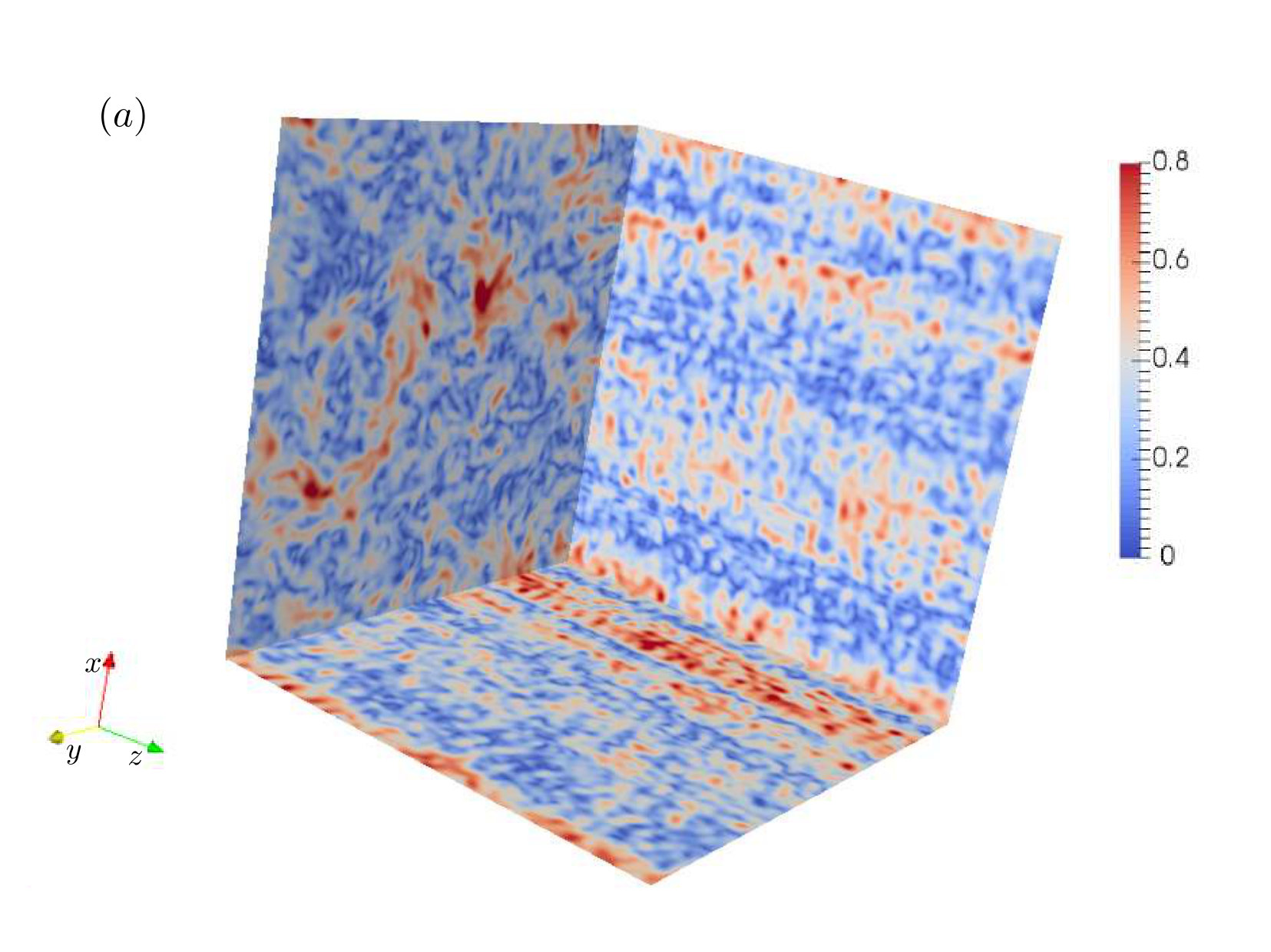 Figure 10
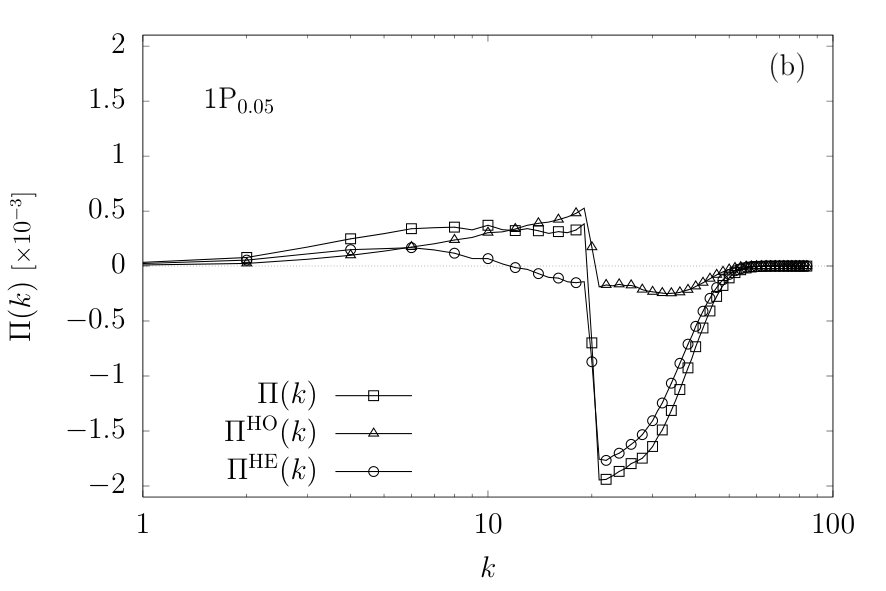 Figure 10
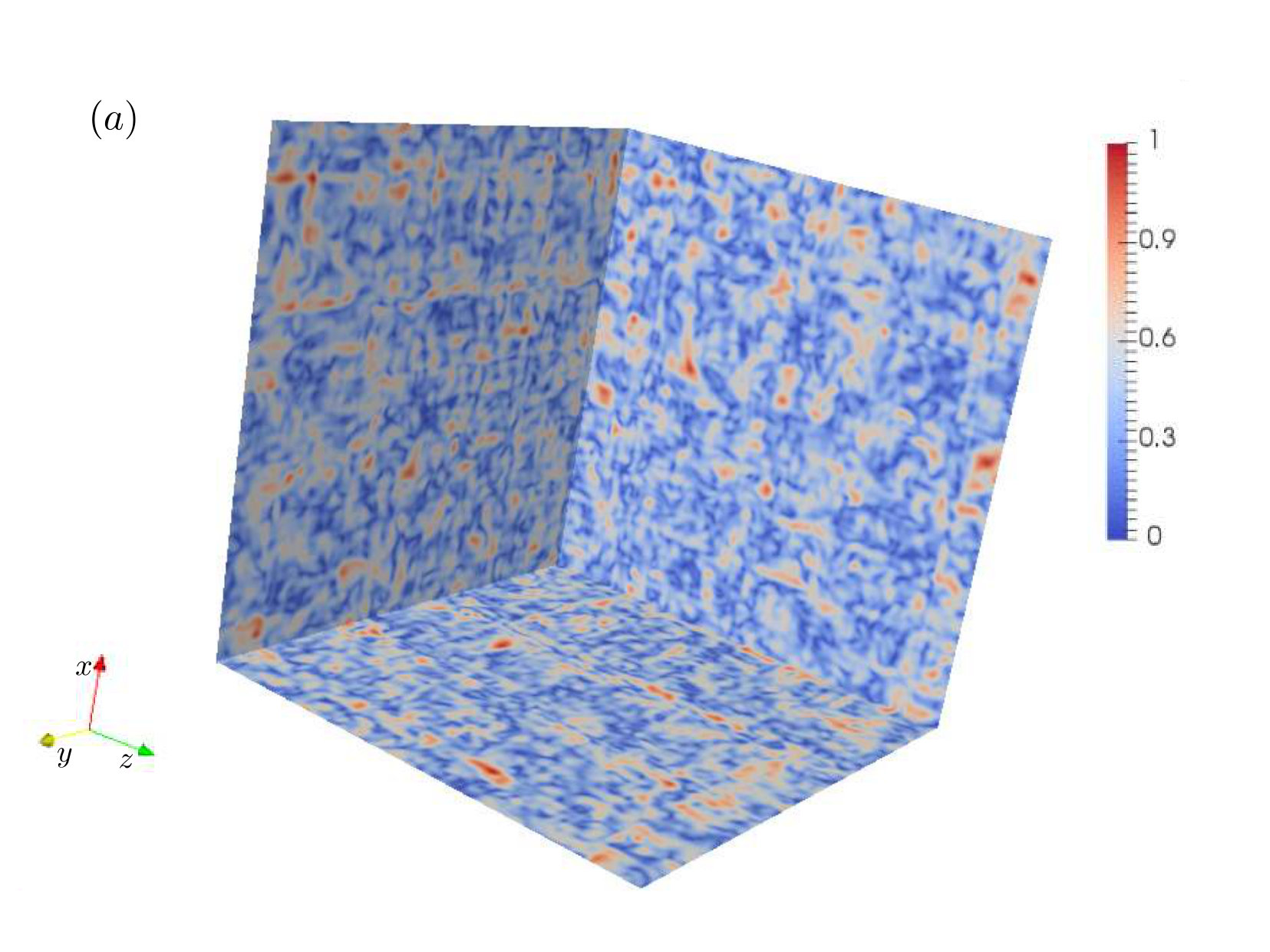 Figure 11
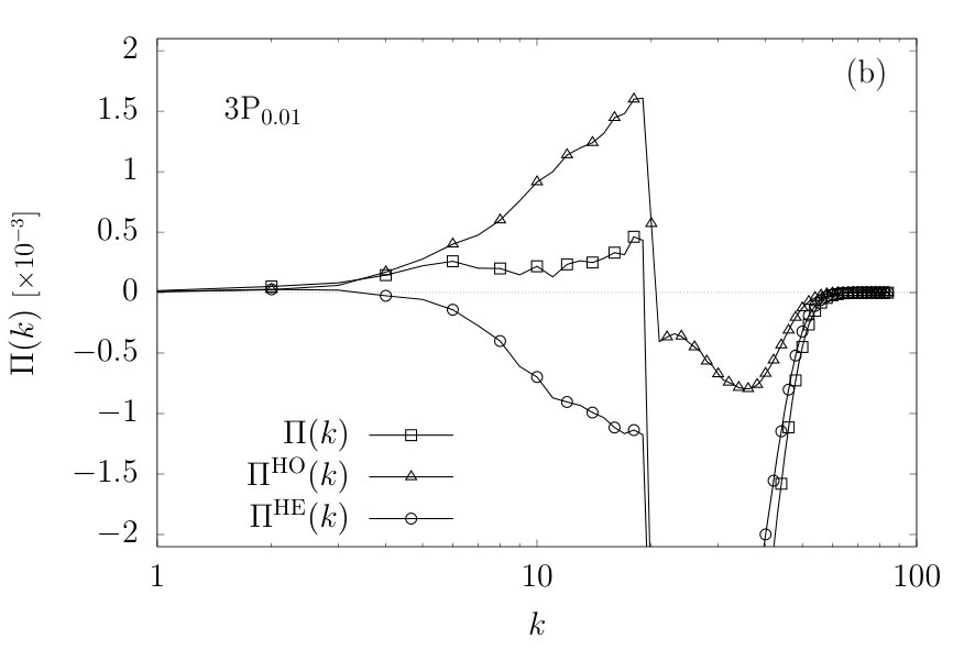 Figure 11
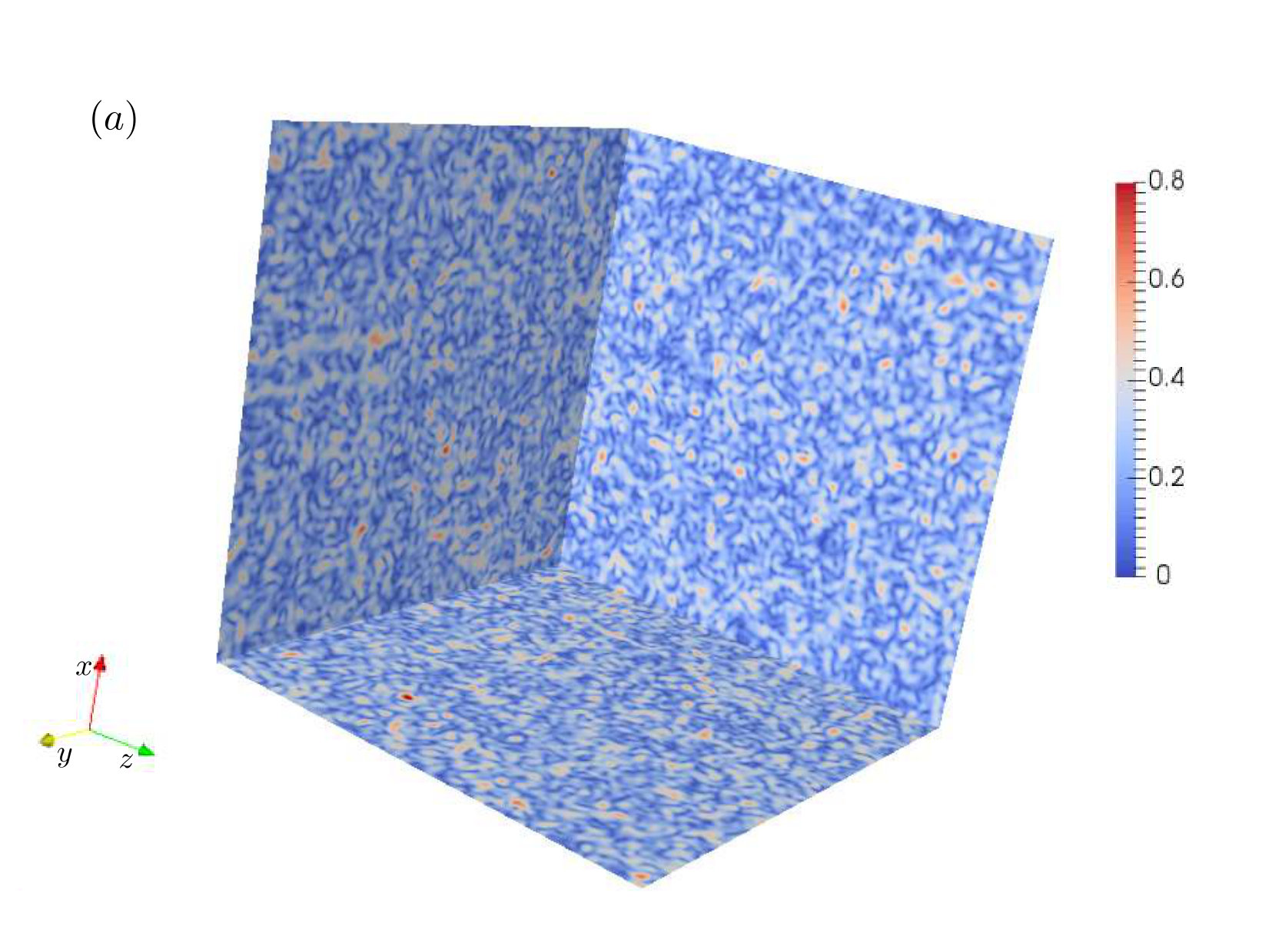 Figure 12
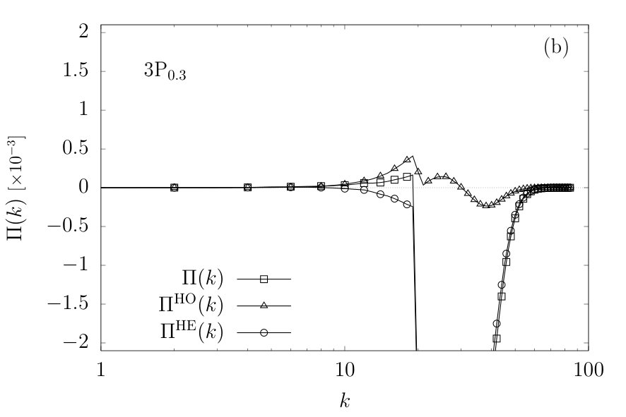 Figure 12
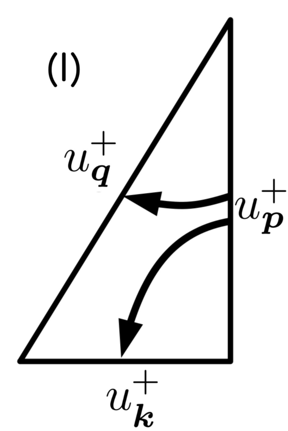 Figure 1
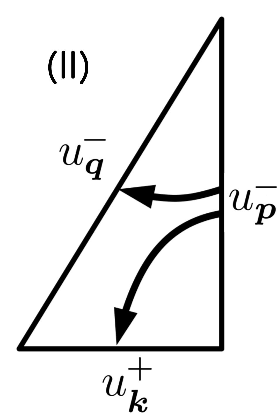 Figure 1
 Figure 1
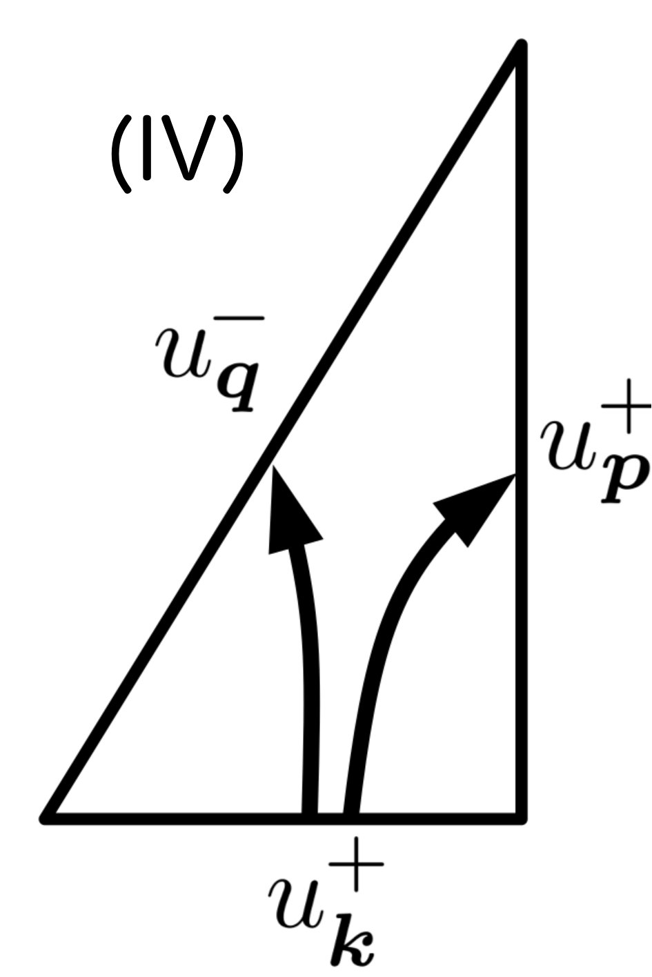 Figure 1
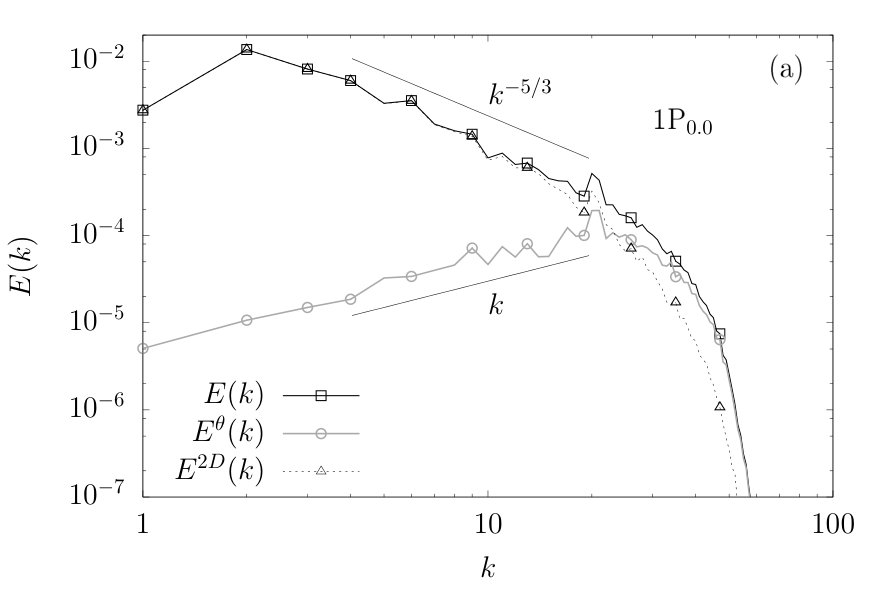 Figure 2
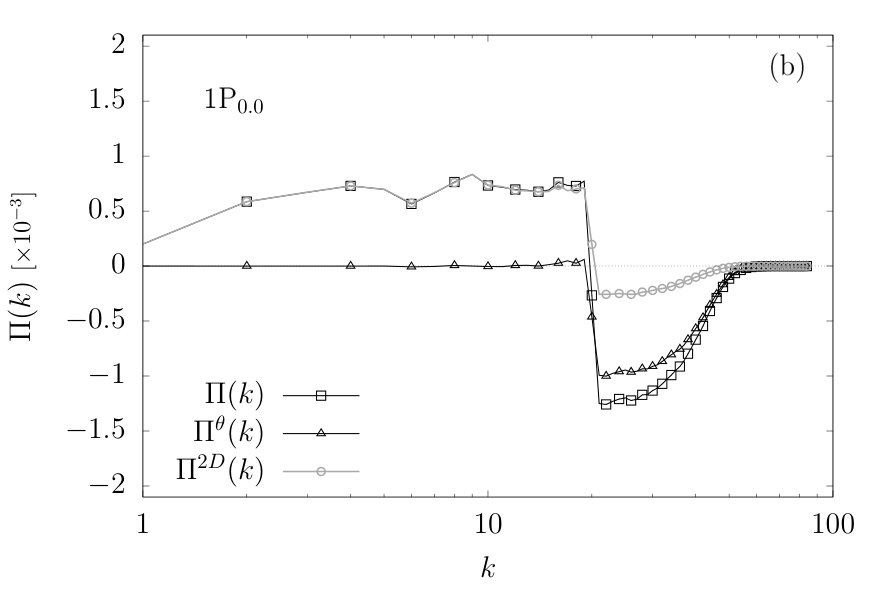 Figure 2
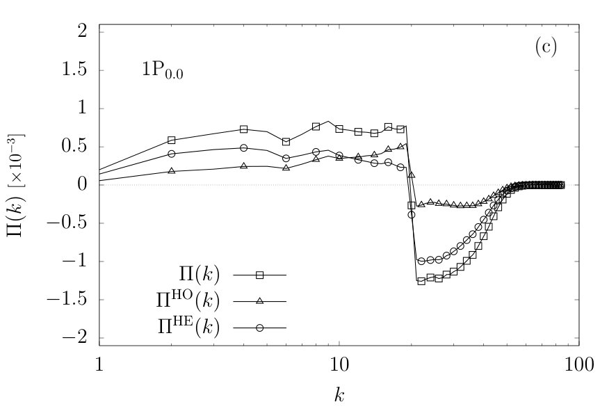 Figure 2
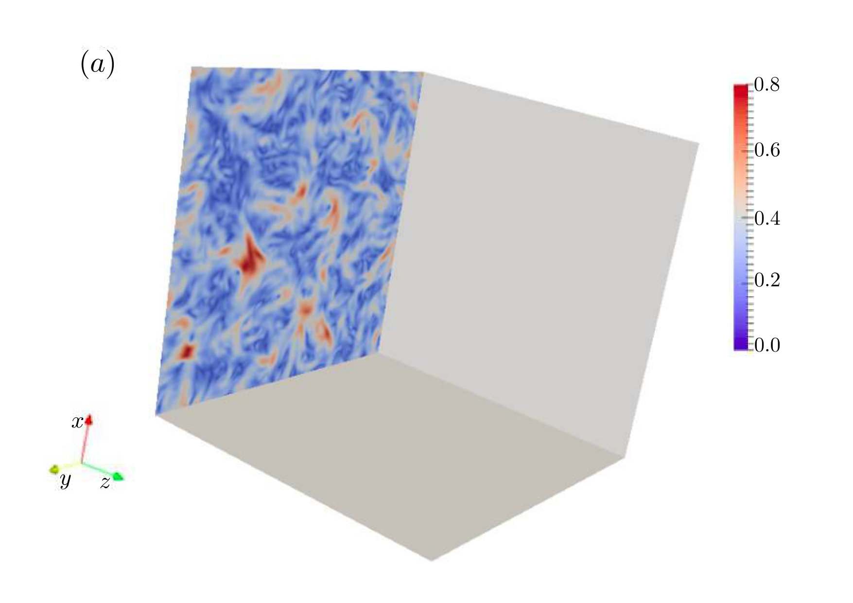 Figure 3
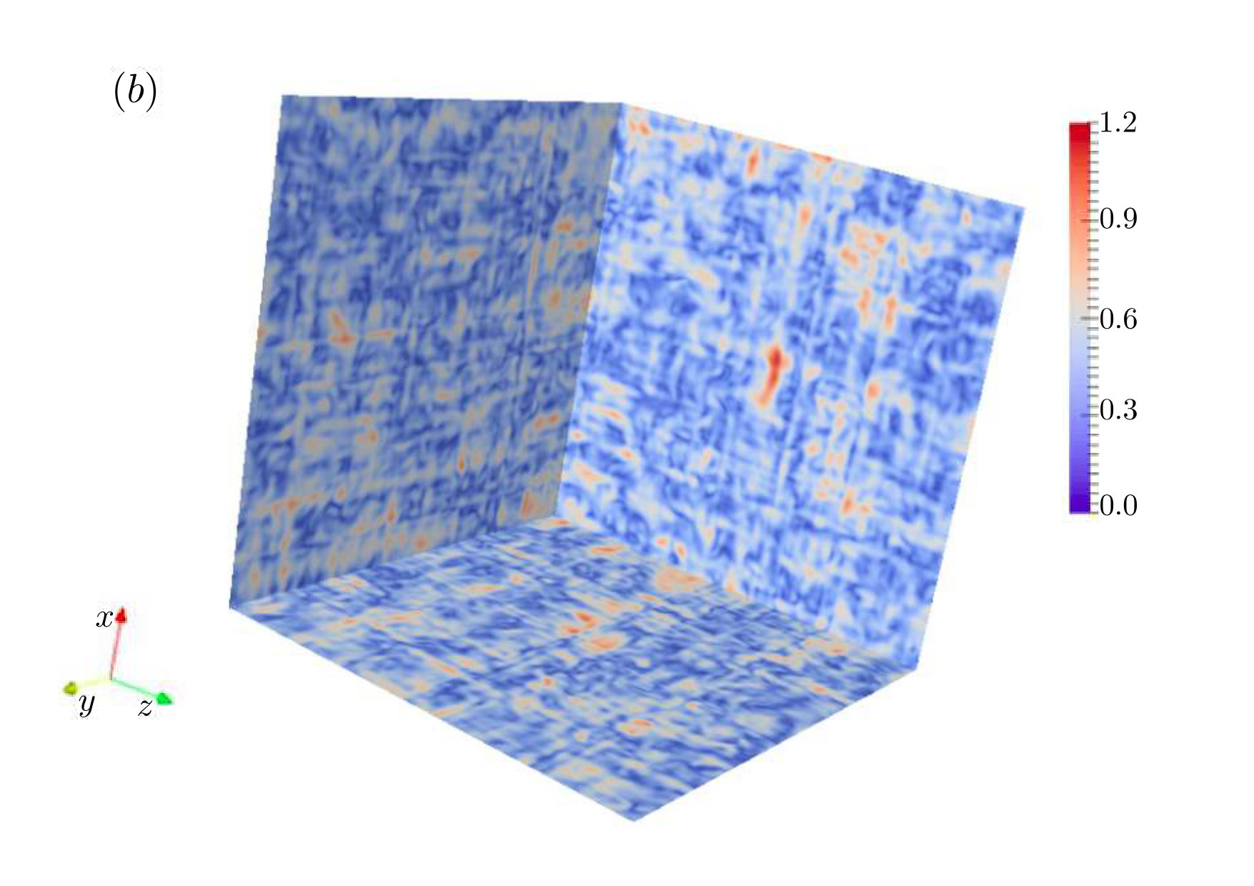 Figure 3
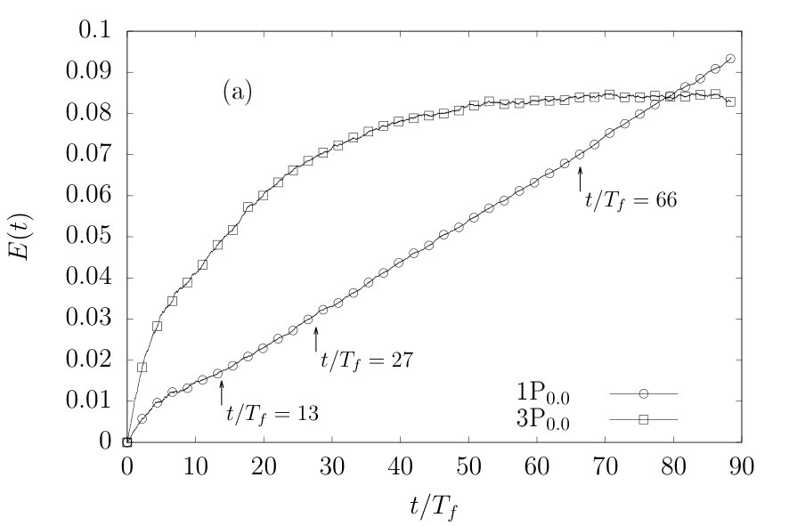 Figure 4
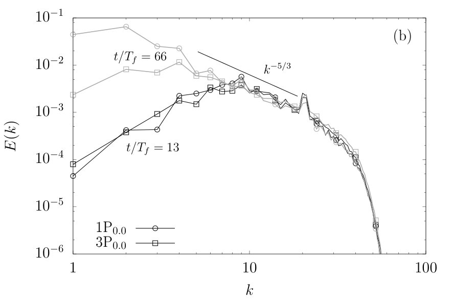 Figure 4
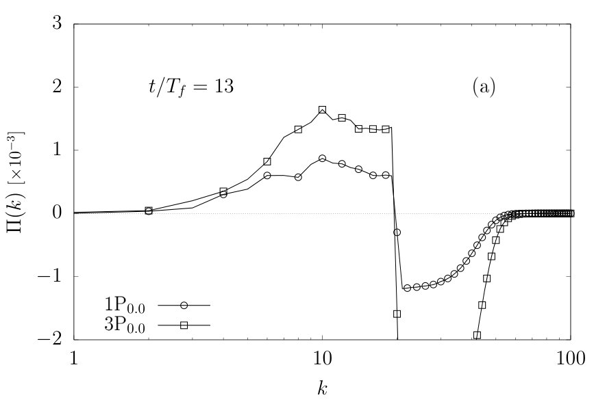 Figure 5
 Figure 5
 Figure 5
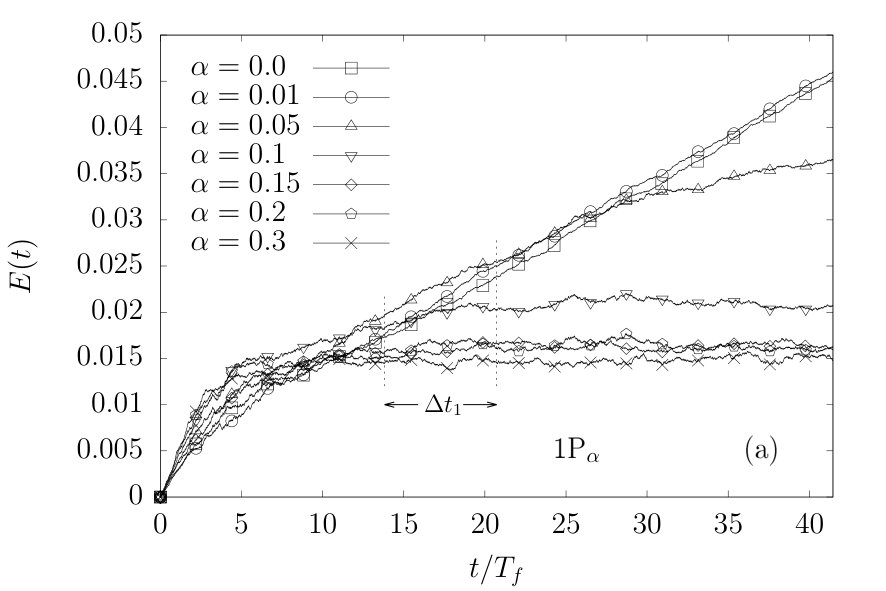 Figure 6
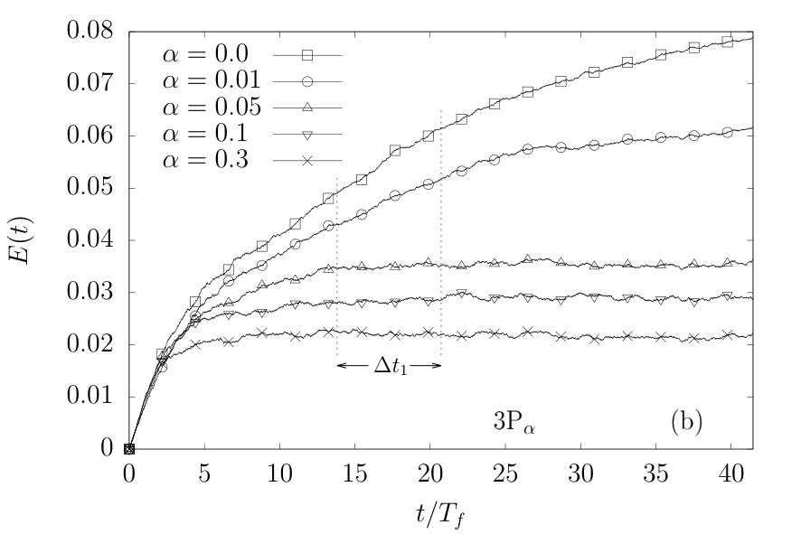 Figure 6
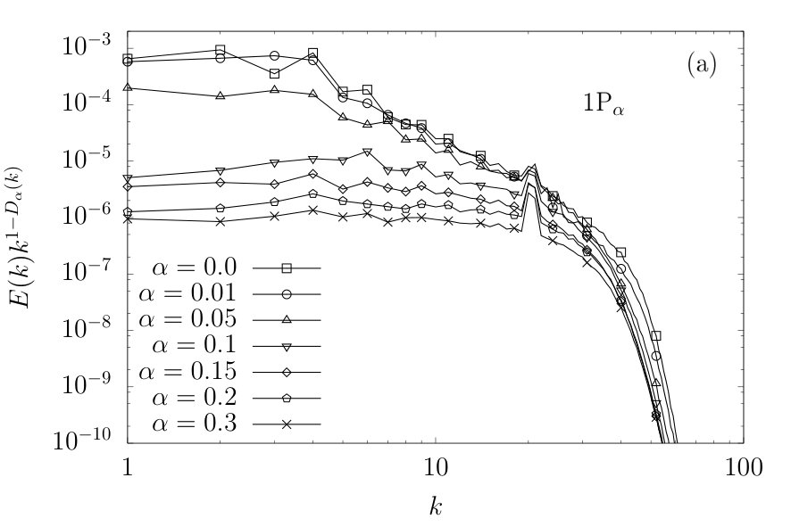 Figure 7
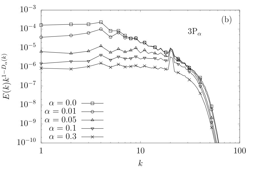 Figure 7
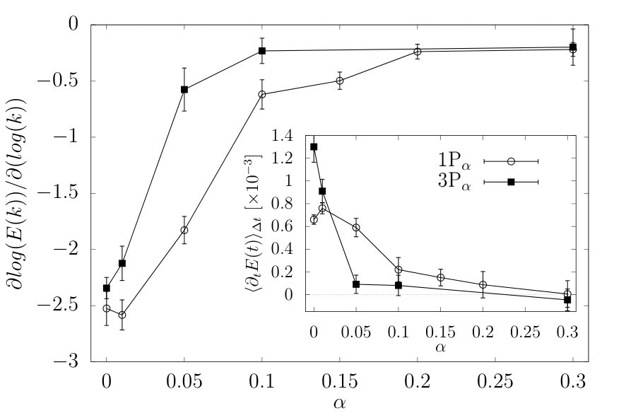 Figure 8
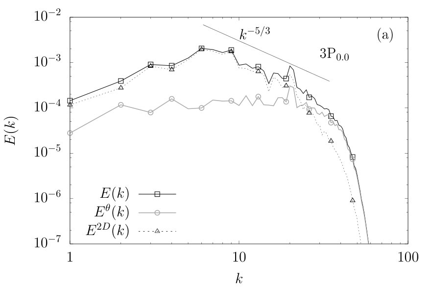 Figure 9
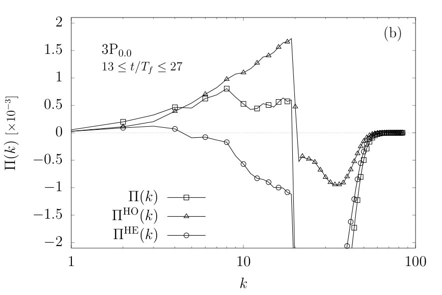 Figure 9
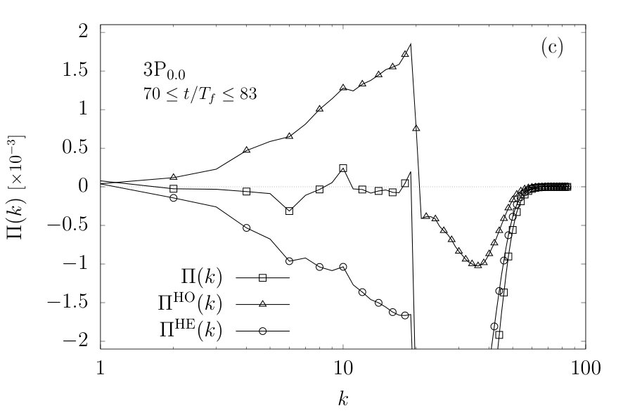 Figure 9
| 1P0.0 | 1P0.01 | 1P0.05 | 1P0.1 | 1P0.15 | 1P0.2 | 1P0.3 | |
| 0.0 | 0.01 | 0.05 | 0.1 | 0.15 | 0.2 | 0.3 | |
| 1.3 | 1.3 | 2 | 2.7 | 2.5 | 3 | 3.2 | |
| 0.42 | 0.42 | 0.33 | 0.2 | 0.18 | 0.18 | 0.17 | |
| 1.2 | 1.2 | 0.7 | 0.18 | 0.15 | 0.132 | 0.128 | |
| 90 | 90 | 90 | 90 | 90 | 90 | 90 | |
| 3P0.0 | 3P0.01 | 3P0.05 | 3P0.1 | 3P0.15 | 3P0.2 | 3P0.3 | |
| 0.0 | 0.01 | 0.05 | 0.1 | - | - | 0.3 | |
| 6 | 6 | 6 | 6 | - | - | 6 | |
| 0.41 | 0.36 | 0.27 | 0.24 | - | - | 0.2 | |
| 0.45 | 0.33 | 0.15 | 0.14 | - | - | 0.128 | |
| 90 | 90 | 45 | 45 | - | - | 45 |
Peer Reviews
No public reviews on file for this paper yet. If you reviewed it on a platform where reviews are public (OpenReview, ICLR, NeurIPS, ICML), you can paste yours below so the community can read it here.
Videos
No videos yet. Explain this paper in a talk, walkthrough, or lecture? Add one.
Postprint version of the manuscript published in Physics of Fluids 29, 111101 (2017).
From two-dimensional to three-dimensional turbulence through two-dimensional three-component flows
L. Biferale
M. Buzzicotti
M. Linkmann
Department of Physics & INFN, University of Rome ‘Tor Vergata’, Via della Ricerca Scientifica 1, 00133 Rome, Italy
Abstract
The relevance of two-dimensional three-components (2D3C) flows goes well beyond their occurrence in nature, and a deeper understanding of their dynamics might be also helpful in order to shed further light on the dynamics of pure two-dimenional (2D) or three-dimensional (3D) flows and vice versa. The purpose of the present paper is to make a step in this direction through a combination of numerical and analytical work. The analytical part is mainly concerned with the behavior of 2D3C flows in isolation and the connection between the geometry of the nonlinear interactions and the resulting energy transfer directions. Special emphasis is given to the role of helicity. We show that a generic 2D3C flow can be described by two stream functions corresponding to the two helical sectors of the velocity field. The projection onto one helical sector (homochiral flow) leads to a full 3D constraint and to the inviscid conservation of the total (three dimensional) enstrophy and hence to an inverse cascade of the kinetic energy of the third component also. The coupling between several 2D3C flows is studied through a set of suitably designed direct numerical simulations (DNS), where we also explore the transition between 2D and fully 3D turbulence.
In particular, we find that the coupling of three 2D3C flows on mutually orthogonal planes subject to small-scale forcing leads to stationary 3D out-of-equilibrium dynamics at the energy containing scales.
The transition between 2D and 3D turbulence is then explored through adding a percentage of fully 3D Fourier modes in the volume.
I Introduction
In his 1967 paper, KraichnanKraichnan67 provided the basis of the current understanding of 2D turbulence. His argument explained the existence of two mutually exclusive inertial ranges corresponding to an inverse energy cascade with an energy spectrum, and to a direct enstrophy cascade with , as well as the formation of a large-scale condensate. The dynamics of the two cascades were predicted to have some important differences, whereby the energy should cascade locally in Fourier space while the transfer of enstrophy proceeds mainly through nonlocal interactions. Both cascades have been observed in experiments and numerical simulations, see e.g. Refs. Lilly69, ; Sommeria86, ; Smith93, ; Paret97, ; Gotoh98, ; Chen03, ; Lindborg00, , and so has the formation of a large-scale condensate in the form of two counter-rotating vortices Hossain83 ; Smith93 ; Smith94 ; Paret98 ; Boffetta10 (see also the recent review in Ref. Boffetta12, and references therein). On the other hand, pure 3D flows have a completely different phenomenology. They develop a forward energy cascade and a build-up of non-Gaussian fluctuations at successively smaller scales Frisch95 . Remarkably enough, there are many instances in nature when the flow is neither 2D nor 3D, enjoying a forward or an inverse energy cascade (or both) depending on the boundary conditions as for the case of thick turbulent layers Celani10 ; Xia11 ; Nastrom84 ; Benavides17 , or on the existence of a strong rotation rate Cambon89 ; Waleffe93 ; Smith99 ; Chen05 ; Mininni09 ; Gallet15a ; BiferalePRX2016 , or on the presence of a strong mean magnetic field Moffatt67 ; Alemany79 ; Zikanov98 ; Gallet15 ; Alexakis11 ; Bigot11 for conducting flows. In all the above instances, the inverse cascade is triggered by a tendency of the flow to become a two-dimensional three-components (2D3C) flow where the third component is passively advected by the two-dimensional flow and the physics is dominated by the inverse energy cascade in the 2D plane. Interestingly enough, recent numerical simulations have also shown that an inverse energy cascade can be sustained by a fully 3D isotropic flow if constrained to evolve only on the subset of homochiral helical Fourier waves Waleffe92 ; Biferale12 ; Alexakis17 , i.e., those of like-signed helicity. In other words there might exist fully 3D structures that bring energy upscale, contrary to what is typically observed for unconstrained 3D turbulence.
Apart from the above-mentioned applications, 2D3C flows might also be relevant for the evolution of fully three-dimensional homogeneous turbulence Waleffe92 ; Moffatt14 . The connection lies in the structure of the inertial term of the Navier-Stokes equations that in Fourier space can be written as the superposition of interactions among three wavevectors and which satisfy the condition to form a closed triad: . Any triad defines a plane in Fourier space, which through a suitable choice of coordinate system can be identified with, e.g., the -plane. The flow corresponding to this single triad of wavevectors is therefore independent of the -coordinate Moffatt14 . Of course, the superposition of many unoriented 2D3C triads is not a 2D3C flows. Hence, there is no a priori reason to believe that the full turbulent evolution of a quasi-isotropic 3D flows has anything in common with the limiting case of a set of co-planar 2D3C triads Moffatt14 .
We can summarize by saying that we know at least two different mechanisms which might trigger a reversal of the energy cascade in a 3D turbulent flow: either the system is pushed toward a 2D (or 2D3C) configuration by some anisotropic external mechanism or it must be constrained to evolve on a strongly helical manifold, with breaking of mirror (but not rotational) symmetry at all scales. The two mechanisms are somehow opposite, helicity being a fully three dimensional quantity.
In this paper we investigate through analytical and numerical methods how one might smoothly go from a pure 2D3C dynamics to a 3D dynamics by successive addition of triads under some controlled protocol. The main interest is to understand how/when the system starts to show 3D behavior and what the main physical mechanisms are that trigger the transition.
For this purpose we first analyze the 2D3C dynamics, which in fact is characterized by a split energy cascade, where the passively advected third component undergoes a direct energy cascade while the advecting flow shows an inverse energy cascade. In order to better understand the split cascade we express the velocity field in two different bases. We use either
the standard decomposition of a pure 2D flow plus a component passively advected or the decomposition in positive and negative helical Fourier waves Constantin88 ; Waleffe92 that will be the building block of any 3D dynamics.
Understanding the relation between the two bases will prove helpful in the description of the physics of the transition from 2D3C to 3D behavior, as the characteristic split cascade of a 2D3C flow will be obscured in the presence of 3D dynamics.
In order to understand the transition to a 3D flow we first study the dynamics of a flow that evolves on three 2D3C manifolds defined on mutually orthogonal planes. As a result we obtain a flow that has the discrete rotational symmetries of the cube and which is mainly based on three weakly coupled 2D3C evolutions. Successively we start to add a percentage of Fourier modes randomly (but quenched in time) in the whole 3D cube and we study the transition to a full 3D isotropic dynamics at increasing . We show that the basic 2D3C flow can be described by introducing two independent stream functions, , which are connected to its helical decomposition. We also found that imposing the homochiral constraint on the dynamics will force one of the two stream functions to be identically zero and the 2D3C dynamics to collapse on a constrained configuration where the component out of the plane is not a simple passive scalar anymore, and that this has important consequences for the global energy transfer. Finally, we study the transition from 2D to 3D dynamics as a function of the percentage of added 3D modes, and we assess the dynamical relevance of the energy transfer due to homochiral triads in the fully 2D3C configuration and for different .
This paper is organized as follows. In section II we discuss the basic setup and review the inviscid invariants particular to 2D3C flows as derived in Ref. Moffatt14, . Section III contains the main part of the theoretical work on the helical decomposition of 2D3C flows, where the description of a 2D3C flow in terms of two stream functions is introduced and the helical decomposition is used to study the effect of different helical interactions on the dynamics of the planar and perpendicular components of the velocity field. The numerical simulations are described in Section IV, beginning with a comparison between the dynamics of single and coupled 2D3C flows. Subsequently we investigate the transition from 2D to 3D turbulence in Section IV.2 and the behavior of a subset of helical interactions leading to an inverse energy cascade in Section IV.3. We summarize our results in Section V.
II Structure and inviscid invariants of the 2D3C Navier-Stokes equations
We start from considering a 2D3C solenoidal velocity field on a three-dimensional domain with periodic boundary conditions, where , and are functions of only and . We define the 2D-component and the component perpendicular to the -plane as to stress that it behaves as a passive scalar (see below)
[TABLE]
such that the total vector field is given by . For such a 2D3C flow, the 3D Navier-Stokes equations split into the 2D Navier-Stokes equations for , while is passively advected
[TABLE]
where is the two dimensional pressure and the kinematic viscosity. For the vorticity the decomposition of into and results in
[TABLE]
and for simplicity we define such that the total vorticity vector field is , with denoting the unit vector in the -direction. The 2D3C Navier-Stokes equations (II) in the vorticity formulation then become
[TABLE]
The 3D Navier-Stokes equations have two inviscid quadratic invariants, the total energy
[TABLE]
and the total kinetic helicity
[TABLE]
per unit volume, while the 2D equations have two quadratic invariants, the total 2D energy
[TABLE]
and the 2D enstrophy:
[TABLE]
The 2D3C flow being a particular 3D case, it is immediately clear from Eqs. (II) and (II) that the energy of the passive component is another quadratic invariant for this case
[TABLE]
When discussing the energy transfer of the 2D3C flow it is necessary to distinguish the component of the energy in the plane, , from the component out of the plane . The former is known to develop an inverse cascade, while the latter is typically transferred to small scales. Hence, the transfer of the total energy can be either forward or backward. For later purpose it is important to remark here that the above conservations hold in Fourier space also on a triad-by-triad basis Moffatt14 . Helicity for the 2D3C case must play a passive role concerning the independent 2D dynamics. Indeed, it is easy to realize that it can be further decomposed in two quantities
[TABLE]
since and . Using Eqs. (II) and (II) it can also be shown that and are conserved and related to each other by a geometrical constraint
[TABLE]
since due to the periodic boundary conditions. Hence, a 2D3C-flow has four inviscid quadratic invariants, where for one of which, the total helicity, the planar and perpendicular components are identical Moffatt14 and passive concerning the evolution of .
III Helical decomposition of a 2D3C flow
Even though helicity is a passive quantity for a pure 2D3C dynamics, it is useful to further disentangle its dynamics in view of the possibility to build up a full 3D flow by adding different 2D3C submanifolds. To do that, we exploit the decomposition of any incompressible 3D flow into helical modes by the procedure proposed in Refs. Constantin88, ; Waleffe92, . Since is a solenoidal vector field, its Fourier modes have only two degrees of freedom, and we have
[TABLE]
where are normalized eigenvectors of the curl operator in Fourier space Constantin88 ; Waleffe92 . The helical decomposition thus decomposes the Fourier modes of the velocity field into two components, each of which satisfies
[TABLE]
and . For a 2D3C flow this requirement becomes
[TABLE]
and we obtain
[TABLE]
where the symbol in the third component of stands for .
III.1 Introduction of two stream functions
For each helical sector we can now define two stream functions through their respective Fourier transforms
[TABLE]
such that are Hermitian-symmetric and
[TABLE]
where the helical basis vectors are given as
[TABLE]
A 2D3C-flow can therefore be described in real space by two stream functions and
[TABLE]
such that
[TABLE]
It is important to stress that we are just changing basis, we move from the usual description in terms of the couple of functions , describing the stream function of the field and the out-of-plane passive component to a couple of fully 3D structures that also reconstruct the original 2D3C flow. While the formulation is natural for the study of turbulence under rapid rotation, passive scalar advection in 2D turbulence or for thick layers of fluid, the helical formulation is the natural decomposition for fully 3D flows. Clearly, there exist two possibilities to reduce the complexity of a 2D3C flow, either through requiring (i) , or, (ii) by setting one of the helical stream function to zero, , say. The entire evolution of the flow in both cases is given by one stream function only, and the quantities , , and are obtained through taking the appropriate derivatives of the single stream function. In the first case where the flow is fully 2D as , and the inner product then vanishes identically. That is, a 2D3C flow with vanishing pointwise helicity is a 2D flow. In the second case where , say, the inner product at all times, hence the flow must be 3D and correlates with at all times. The two cases bear the important difference that the latter case is dynamically unstable while the former is not. The flow in case (i) which is initially 2D will remain so unless it is subjected to 3D perturbations, while in case (ii) negatively helical Fourier modes are always created through nonlinear interactions. In order to maintain a flow in case (ii) where at all times, it is necessary to re-project the evolution onto the submanifold corresponding to alone.
Separate evolution equations for and can be obtained from the respective evolution equations for and (we neglect the dissipative terms from now on)
[TABLE]
which leads to the usual equation of the 2D stream function when
[TABLE]
Also in the fully helical case, , the flow is again described by one stream function only. However, the evolution of the single stream function derived from Eq. (III.1) differs in this case from that of a 2D flow given by Eq. (24)
[TABLE]
As discussed before, the removal of one degree of freedom in the helical decomposition forces the perpendicular component to be correlated to the 2D vorticity . In this case does not evolve anymore as a passive scalar with important consequences for the cascade direction of its energy , as discussed in the following section.
III.2 Cascade directions and helical interactions
The inviscid invariants can be expressed in terms of the Fourier transforms of and
[TABLE]
while the enstrophy in the plane can be written as
[TABLE]
For a fully helical velocity field (), we have that and . As a result also the ‘enstrophy’ of the field is conserved leading to an inversion of the direction of the transfer. Thus, for 2D3C homochiral evolutions, the total energy will necessarily be transferred upscale because also the ‘passive’ component does not behave anymore as a passive scalar in 2D and will develop an inverse energy cascade. The latter observation also implies that a forward cascade of in the full 2D3C case can only occur through interactions between and (see also Appendix B). The above energy transfer property of homochiral triads was already discussed in the original paper by Waleffe Waleffe92 and it is at the basis of the numerical simulations of homochiral turbulence developed in Refs. Biferale12, ; Biferale13, ; Sahoo15, resulting in 3D fully isotropic turbulence with an inverse cascade. Here we stress the connection with the underlying 2D3C structure of any isolated triadic Navier-Stokes interaction and the important remark that in such a case the direction of the transfer of the total energy can always be decomposed in two contributions, one due to the transfer of the 2D physics (always inverse) and one due to the amount of energy transferred by the out-of-plane components, which is typically forward and only backward if we restrict to homochiral dynamics.
In this context it is interesting to notice that in a rotating fluid Ekman pumping near a solid boundary leads to a vertical velocity component which is directly proportional to the vertical vorticity component, that is, to a flow with pointwise positive helicity everywhere close to the boundary. The result is an effective reduction in the number of degrees of freedom, because in terms of the helical decomposition the resulting flow would be described by one helical stream function only. In consequence, the vertical velocity component close to the boundary in a rapidly rotating flow should display an inverse energy cascade.
III.3 Fourier decomposition
In order to shed some further light on the couplings between the two stream functions, their respective contributions to the 2D dynamics and the dynamics of the perpendicular component, we consider the evolution of the Fourier transforms of and
[TABLE]
which are obtained directly from the Navier-Stokes equations in Fourier space by first substituting the general helical decomposition for a 3D velocity field Waleffe92 and subsequently using Eq. (18). Here , as the inertial term has been written in rotational form.
After some algebra (see Appendix A) it is possible to obtain the evolution equations for the stream functions in the helical decomposition with planar and perpendicular contributions written separately
[TABLE]
since the coupling factor
[TABLE]
consists of a contribution coming from the 2D dynamics and one coming from the dynamics of the perpendicular component.
We now consider homo- and heterochiral helical interactions separately. A homochiral interaction has by definition , while a heterochiral interaction must have both signs of helicity. All possible helical triad interactions present in the Navier-Stokes equations are depicted in Fig. 1, where without loss of generality we only consider . Homochiral interactions correspond to triads of Class (I) in Fig. 1 and are known to produce an inverse energy cascade Waleffe92 ; Biferale12 ; Biferale13 . Heterochiral triads correspond to Classes (II-IV) in Fig. 1, where Classes (III) and (IV) lead to a direct cascade while the energy transfer direction deduced from Class (II) depends on the geometry of the triad. The peculiar behavior of Class (II) triads had already been inferred by WaleffeWaleffe92 , it has since been confirmed in numerically using shell models DePietro15 . Class (II) triads also possess further inviscid invariants which are geometry-dependent and determine the direction of the energy transfer Rathmann16 .
III.3.1 Homochiral interactions
For (Class (I)), the coupling factors become
[TABLE]
and since the triangle inequality implies that the term corresponding to 2D dynamics is larger than the term corresponding to the dynamics of the perpendicular component, we conclude that homochiral interactions mainly contribute to the 2D dynamics. The weighting of planar and perpendicular parts of the coupling factor implies that the extra term which appears in the homochiral case in the evolution equation (III.1) of the stream function is subdominant. This suggests that a homochiral 2D3C flow has similar dynamics compared to a fully 2D flow, which is also reflected in the fact that despite being not fully 2D, it conserves the total enstrophy.
III.3.2 Heterochiral interactions
For (Classes (III) and (IV)), the coupling factors become
[TABLE]
and since the triangle inequality implies , the term corresponding to 2D dynamics is smaller in magnitude than that corresponding to the dynamics of the perpendicular component. Hence we conclude that these heterochiral interactions mainly contribute to the dynamics of the perpendicular component.
The final case to consider is a heterochiral interaction of Class (II), where . In this case, the coupling factor becomes
[TABLE]
and we see that this type of interaction behaves differently from the other heterochiral interactions. Similar to the homochiral case, the triangle inequality implies that the term corresponding to 2D dynamics is larger than the term corresponding to the dynamics of the perpendicular component. Hence we conclude that this particular type of heterochiral interaction mainly contributes to the 2D dynamics.
III.3.3 Discussion
In contrast to the fully 3D case, the coupling factor corresponding to the 2D evolution (see also eq. (A) in Appendix A) is helicity-independent. This has two consequences:
(i) in 2D () all couplings between the stream functions (i.e. all helical interactions) are equally weighted for a given triad geometry,
(ii) a stability analysis based on single triads corresponding to 2D dynamics extracted from Eq. (32) gives the same results for all helicity combinations as shown in Ref. Waleffe92, .
In 2D all interactions therefore lead to an inverse energy cascade and the coupling factor is the same. That is, all classes of helical interactions produce an inverse energy cascade when restricted to the evolution in the plane. Concerning the evolution of the perpendicular component, the coupling factor is helicity-dependent in such a way that helical interactions leading to a forward cascade (Classes (III) and (IV)) are higher weighted than those leading to an inverse energy cascade or a mixed energy transfer (Classes (I) and (II)). This confirms that a passive scalar in 2D turbulence should display a direct energy cascade, in accord with the known phenomenology of passive scalar advection in 2D Falkovich01 , see Appendix B for a further discussion of this point.
Figure 2(a-c) presents the energy spectra of the planar and perpendicular components
[TABLE]
and the corresponding fluxes
[TABLE]
of the single 2D3C flow and the total, homo- and heterochiral energy fluxes
[TABLE]
respectively. The data has been obtained by DNS of a 2D3C flow as described in detail in Sec. IV. From Fig. 2(a) we observe clearly the predicted behavior of the 2D and the perpendicular component with displaying an inverse-cascade -scaling while shows equipartition scaling in the same wavenumber range. As a result, the total energy spectrum at is mainly given by the 2D component. The separate fluxes and are shown in Fig. 2(b), which confirms that the inverse energy flux is exclusively generated by the 2D dynamics, while the perpendicular component has zero inverse flux in agreement with the 2D absolute equilibrium scaling of its energy spectrum shown in Fig. 2(a). Interestingly enough, concerning the energy flux in the helical decomposition, the inverse cascade of total energy is given to a large extent by the homochiral fluxes according to Fig. 2(c), which is consistent with the analysis presented in Sec. III.2, since homochiral interactions mainly contribute to the evolution in the plane. However, the homochiral flux is not reproducing the total energy flux entirely and heterochiral interactions also contribute to the inverse flux at all scales larger than the forcing scale, as expected for 2D dynamics which must be helicity-insensitive. A more remarkable difference between homo- and heterochiral components of the flux is detectable for scales smaller than the forcing scale, where the homochiral contribution is fully negligible.
Notice that accounts for nearly one-third to one-half of for (see Fig. 2(c)), which according to Fig. 2(b) is given by the 2D dynamics only. However, the geometry of the nonlinear coupling in the plane suggests that the homo- and heterochiral contributions to the planar dynamics are identical, and one would expect if the dynamics was purely 2D. However, the heterochiral contribution to is mostly forward (in the wavenumber range ), hence we expect less energy to be transferred upscale by heterochiral interactions compared to homochiral interactions. In summary, homochiral interactions enhance the 2D physics and lead to a better inverse cascade in 2D3C flows than heterochiral interactions.
IV Numerical Simulations
The analytical results shed some light on the fundamental properties of the 2D3C Navier-Stokes equations by disentangling the dynamics of the plane from that of the perpendicular component, and they provided some qualitative results concerning the particular dynamics of homochiral interactions. However, in order to study their effective importance for realistic 3D or quasi 3D flows, we need to perturb the basic 2D3C flows. We do it in different steps. First we start by coupling three 2D3C flows each one restricted on one of the three perpendicular planes , and . The resulting dynamics is not a simple superposition of the three 2D3C dynamics because there will be triads that couple the three planes. Hence, we expect to have a mixture of 2D and 3D phenomenology, depending on the relative weights of triads fully contained in each one of the three planes and triads with vertices on at least two different planes. In particular, the additional inviscid invariants specific to single 2D3C flows are no longer conserved, and the only inviscid invariants of the coupled 2D3C flows are those of the full 3D Navier-Stokes equations, i.e., the total energy and the kinetic helicity. Furthermore, the splitting into two stream functions is not possible any longer.
We carry out two series of simulations, series 1P refers to the base flow being a single 2D3C flow in the -plane while series 3P consist of three 2D3C flows as the base configuration.
Furthermore, we will also successively decorate both sets of base flow by adding randomly (but quenched in time) modes that are fully 3D, i.e. taken blindly in the 3D Fourier space. By changing the percentage to have modes we will be able to move from where we have either the 1P or 3P configuration to a fully resolved 3D Navier-Stokes case when . We will mainly look for a change in the cascade direction from inverse (2D) to direct (3D), leaving to further studies other important issues as, e.g., the impact on small-scale intermittency. In order to do that we always force the system at small scales and to achieve a large scale separation while still resolving some small-scale turbulence, we use higher order hyperviscous Navier-Stokes equations
[TABLE]
where denotes the velocity field, the pressure, the (hyper)viscosity, an external force and the power of the Laplacian. Equations (45)-(46) are stepped forwards in time using a pseudospectral code with full dealiasing according to the two-thirds rule Patterson71 on collocation points in a triply periodic domain of size , such that the smallest resolved wavenumber is and the largest resolved wavenumber is . The external force is given by a -correlated random process in Fourier space
[TABLE]
where is a projector applied to guarantee incompressibility and is nonzero in a given band of Fourier modes concentrated at intermediate to small scales . The magnitude of the forcing and the value of the hyperviscosity are the same for all simulations. Depending on the type of simulation, Eqs. (45)-(46) are Galerkin projected on the appropriate subspaces, i.e. the -plane in isolation or the , and -planes only. The same can be done when we randomly add modes in the whole Fourier space. This is achieved through a probabilistic projector acting on the velocity field Frisch12 ; Lanotte15 ; Buzzicotti16 in the volume outside the planes
[TABLE]
where
[TABLE]
for . The projector is determined at the start of the simulation and remains unchanged afterwards. In order to guarantee that the evolution of the projected field remains in the same subspace , the nonlinear term in the Navier-Stokes equations must be re-projected at each iteration step.
A summary of specifications of the simulations including the chosen values of is provided in table I. In the following we will use the short-hand notation and to indicate simulations starting from a basic 1P or 3P configuration with a given value of .
IV.1 3 Coupled 2D3C-flows
Before discussing the effect of additional 3D modes, we describe the evolution of the two base configurations and , that is, a single 2D3C flow and three coupled 2D3C flows. The single 2D3C flow is expected to display an inverse cascade of the 2D component while the third component evolves as a passive scalar. The coupled 2D3C flows should also display an inverse cascade corresponding to decoupled or weakly coupled 2D3C dynamics. However, although the three planes may be weakly coupled at small scales, at the large scales, i.e. small , the coupling will become more significant due to a larger relative fraction of triads coupling wavevectors of the three planes. Hence, their coupling should produce 3D dynamics and the inverse cascade is expected to stop, leading to a transient inverse energy transfer which does not lead to the formation of a large-scale condensate. This is exactly the opposite of what typically happens in geophysical flows, where the small-scale dynamics is almost 3D and only the large scale evolution is feeling the 2D confinement. Our three-plane 2D3C configuration has a reverted behavior.
The time evolution of the total energy for configurations and is shown in Fig. 4(a), and we clearly observe that the kinetic energy of the single 2D3C flow grows linearly, which is a tell-tale sign of an inverse energy cascade, while the coupled 2D3C dynamics results eventually in the formation of a stationary state as expected. Figure 4(b) shows the total energy spectra corresponding to snapshots at and in the time evolution of both configurations corresponding to the arrows in Fig. 4(a). As can be seen, both configurations show an inverse cascade -scaling at , which it stops around for run while it continues to larger scales for run , as expected. Visualizations of the two base configurations are shown in Fig. 3, where it can be seen that the single 2D3C dynamics results in the formation of large-scale structures while that of the coupled 2D3C dynamics does not.
The energy fluxes for both configurations are shown in Figs. 5(a-c) at , and , respectively. At early times in the evolution () we observe a clear inverse energy flux in both runs. As can be seen by comparison of the three figures, the inverse flux remains for run , while it diminishes as run approaches the stationary state. Figure 5(c) corresponds to a snapshot in time after saturation of run , and we observe that the inverse flux corresponding to run now nearly vanishes. In the present setup this does not imply that no energy is transferred into the large scales, since the corresponding energy spectrum shown in Fig. 4(b) has not transitioned to an equipartition spectrum as would be the case for a fully 3D flow subject to small-scale forcing Dallasetal15 . As such, the absence of a pronounced inverse flux must result from a balance between inverse and forward fluxes leading to a stationary state and it cannot be interpreted as a sign of a transition to fully 3D dynamics. The latter point is further discussed in the context of the contribution of homo- and heterochiral contributions to the total flux in Sec. IV.3.
IV.2 2D-3D transition
Having described the main features of the base configurations and , we now proceed to an investigation of the transition to fully 3D dynamics in both configurations. The time evolution of the total energy for each run in the two DNS series 1P and 3P corresponding to different percentage of added 3D Fourier modes is presented in Fig. 6(a) and (b), respectively. For both series we observe that by increasing a stationary state is reached earlier in time and with a lower total energy. Furthermore, in both cases no significant difference in the evolution of the total energy can be seen already for and larger. For series the results shown in Fig. 6(a) suggest that the transition from 2D to 3D dynamics appears to occur at , as run does not show any transient inverse transfer while run shows initially an inverse energy transfer which saturates around . In contrast, the transition occurs faster as a function of for series 3P, as run reaches a stationary state at already and run does not display an inverse energy transfer at all.
These results are further substantiated by measurements of the energy spectra for the two series of DNSs obtained either during stationary state where applicable, or otherwise by time averaging over a short interval at late times in the simulation. The shape of the energy spectrum at wavenumber depends on the dimensionality of the flow and the direction of the energy flux. In particular, in fully 3D dynamics the absence of an inverse total energy flux results in the Fourier modes in the range being in statistical equilibrium with equally distributed kinetic energy amongst them Hopf52 ; Kraichnan73 ; Dallasetal15 . Any residual inverse energy flux will perturb this equilibrium state and hence will result in deviations from the expected scaling of the energy spectra. Figures 7(a) and (b) show the energy spectra for series 1P and 3P, respectively, compensated with the absolute equilibrium prediction corresponding to the fraction of added 3D modes
[TABLE]
where for , for , while for the value of is determined numerically by brute force counting the number of active modes in a given wavenumber shell. As can be seen from Fig. 7(a), run is not in equilibrium yet while is. For series 3P, according to Fig. 7(b) run is already in equilibrium while is not. A quantitative difference between the two cases could be expected due to the presence of a larger number of possible 3D triads that can form in series 3P compared to series 1P.
In order to describe the transition from 2D to 3D turbulence more quantitatively, we determine the deviation of the respective energy spectra from absolute equilibrium scaling as a function of . For this purpose the slopes of the compensated energy spectra shown in Fig. 7 for different values of have been measured through least-squares fits with results shown in Fig. 8 for both series of simulations. The results presented in the figure place the value of at which the transition occurs in the range for series 3P and in the range for series 1P. In Appendix C we present a rough theoretical argument predicting the critical value based only on the geometric structure of the nonlinearities for the configuration. The inset of Fig. 8 shows measurements of the time-derivative of the total energy for all runs from series 1P and 3P, where indicates the presence of an inverse cascade while is satisfied in the stationary state. Angled brackets denote a temporal average. Owing to the saturation effect that occurs eventually even in the base configuration , the measured values of depend on the interval the time-derivative is averaged over.
Visualizations of the flows obtained by adding a fraction of 3D modes to the two base configurations are shown for both series in Figs. 10(a)-12(a), where Fig. 10(a) corresponds to a single 2D3C flow with () while Fig. 11(a) shows to a three coupled 2D3C flows with (). The respective values of correspond to perturbed 2D3C flows before the transition to 3D dynamics has taken place. From Fig. 10(a) we observe that the flow now shows some variations along the -axis, however, the main features of 2D evolution such as the formation of large-scale structures, are still visible. In contrast, the coupled 2D3C flows with presented in Fig. 11(a) shows no such structure, although the characteristic pattern of the coupled 2D3C dynamics is still visible.
IV.3 Homo- and heterochiral subfluxes during the 2D-3D transition
In this section we investigate the behavior of the energy subfluxes corresponding to homo- and heterochiral interactions during the transition from 2D to 3D turbulence. According to the arguments presented in Sec. III.2, it can be expected that the qualitative behavior of the homochiral subfluxes remains unaltered during the transition while the heterochiral subflux should visibly change.
Figure 9(a) presents and for one of the three planes. As can be seen, unlike for a single 2D3C flow shown in Fig. 2(a), is no longer in equipartition. Furthermore, now only shows a partial inverse-cascade -scaling at . Both observations are consistent with the coupled 2D3C flow becoming partly 3D. This is also reflected in the fluxes , and shown in Fig. 9(b) before saturation and in Fig. 9(c) after saturation. We now observe that dominates the total flux at intermediate scales while has changed from 2D to 3D behavior, leading to cancellations between the two and hence a lower total inverse energy flux compared to the single 2D3C case where all helical combination lead to an inverse cascade (see Fig. 2(c)). After saturation the homo- and heterochiral subfluxes nearly cancel out and the average total inverse flux vanishes. Hence the dynamics of the coupled 2D3C flows is consistent with a qualitative picture of competing 2D and 3D dynamics, even without a further addition of 3D modes in the volume.
The latter is further supported by the observations made from the total, homo- and heterochiral fluxes for runs and shown in Figs. 10(b) and 11(b), respectively, where we also find that the homochiral flux begins to dominate the total energy flux at intermediate scales larger than the forcing scale, while the heterochiral flux is changing sign. In particular for run shown in Fig. 10(b) we observe partial 2D and 3D dynamics at different scales. In summary, the qualitative behavior of the homochiral dynamics is robust under the transition from 2D to 3D turbulence, while the behavior of heterochiral energy transfers changes, leading eventually to a depletion of the total inverse energy flux. The change of the heterochiral interactions is due to more and more out-of-plane couplings becoming available at the large scales, which according to the results in Sec. III.3 dominate over the heterochiral contribution to the inverse energy transfer in the planes. Once the transition to 3D dynamics is complete, all fluxes tend to zero in the wavenumber range as shown representatively in Fig. 12(b) for run . This behavior can be expected, since the heterochiral interactions are transferring energy downscale very efficiently, before any upscale energy transfer due to homochiral interactions can be established.
The results on the behavior of homo- and heterochiral interactions in isolation suggests that homochiral 2D3C subdynamics enhance the 2D physics. They are almost 2D in the sense that they conserve the total enstrophy. Their dynamical role seems to persists during the 2D3C to 3D transition despite the system becoming increasingly 3D and conserving only the usual 3D inviscid invariants and .
V Conclusions
We have investigated the structure and the dynamics of 2D3C flows, which can be seen as the basic building blocks of 3D turbulence, through numerical simulations and analytical work. Using the Fourier helical decomposition, we have shown that any 2D3C flow can be described through two stream functions corresponding to the two helical sectors of the velocity field. As a result, a homochiral 2D3C flow is described by one stream function only. The projection onto the submanifold corresponding to the homochiral dynamics enforces a correlation between the component of the velocity field perpendicular to the -plane and the vorticity of the planar component . Hence a homochiral 2D3C flow can never be purely 2D and ceases to obey the same equations of a passive scalar. The projection operation also results in the inviscid conservation of the total enstrophy, hence the total 3D kinetic energy confined to the homochiral submanifold must display an inverse cascade.
We explore the transition from a 2D3C to a full 3D dynamics by coupling several 2D3C flows through a set of suitably designed direct numerical simulations (DNS).
We found that the coupling of three 2D3C flows on mutually orthogonal planes leads to a stationary regime where due to competing subfluxes . Unlike in full 3D configurations subject to small-scale forcing, the kinetic energy is not equally distributed amongst the Fourier modes at wavenumbers corresponding to scales larger than the forcing scale, and we obtain stationary out-of-equilibrium 3D dynamics at the energy containing scales.
The situation is also the opposite of what typically happens in geophysical situations, here the flow is 2D at high wavenumbers and becomes 3D only at large scales. The transition between 2D and 3D turbulence has been further explored through adding a percentage of 3D Fourier modes in the whole volume. We found that the homochiral sector tends to transfer energy upward always, while heterochiral triads start to transfer energy to small scales as soon as a small percentage of modes occupy the whole Fourier space isotropically. We also present a rough argument based on a geometrical balance of 2D-3D triads to predict such a transition. In conclusions, we have shown that it is possible to shed further lights on the entangled dynamics of 2D-2D3C-3D flows by using a decomposition in helical waves and by performing suitable numerical experiments meant to restrict the dynamics on different submanifolds.
Acknowledgements.
We thank one of the anonymous referees for their interesting remark about Ekman friction in the context of the helical decomposition. The research leading to these results has received funding from the European Union’s Seventh Framework Programme (FP7/2007-2013) under grant agreement No. 339032. We acknowledge very useful discussions with B. Gallet and previous collaborations on similar topics with R. Benzi, P. Perlekar, G. Sahoo and F. Toschi.
Appendix A Geometric factors for 2D and perpendicular evolution equations
In order to separate the evolution in the plane from that in the perpendicular direction, we further decompose the helical basis vectors
[TABLE]
where the projection on the plane
[TABLE]
is helicity-independent and . The perpendicular component carries all information on helicity, it is defined as
[TABLE]
such that , and we define . The planar and perpendicular components of the evolution equation Eq. (III.3) can now be obtained by taking the inner product of Eq. (III.3) with the appropriate basis vector. For the planar component we obtain
[TABLE]
where is the angle between wavevectors and (see below). As expected, the coupling factor is helicity-independent. For the perpendicular component we obtain
[TABLE]
where the coupling factor now depends on the helicities of the stream functions.
The coupling factors are calculated by taking the inner product of with either (2D) or . We first calculate
[TABLE]
For the 2D geometric factor we obtain
[TABLE]
such that the coupling factor in front of in Eq. (A) becomes
[TABLE]
where the triad condition was used in the second step. For the geometric factor in the perpendicular component we obtain
[TABLE]
such that the coupling factor in front of in Eq. (A) becomes
[TABLE]
where the triad condition was used in the second step.
Appendix B Passive scalar evolution in 2D turbulence
The helical decomposition of the 2D3C flow can formally be applied to the dynamics of a passive scalar in 2D turbulence by defining
[TABLE]
where is the stream function of the 2D flow. The decomposition in Fourier space is then
[TABLE]
The Fourier-space evolutions equations for and
[TABLE]
correspond in the helical decomposition to Eqs. (A) and (A), respectively. Following the discussion in Sec. III.2, the passive scalar evolution is therefore dominated by ‘heterochiral’ interactions, which according to the stability arguments in Ref. Waleffe92, would indicate that should display a forward cascade. We note that a direct stability analysis of single-triad dynamical systems derived from Eqs. (62) and (63) in conjunction is not possible because the usual trick using -order time derivatives does not lead to closed equations for the passive scalar. However, for an active scalar it may work. This problem does not arise for triads involving only the stream function, the stability analysis for the 2D dynamics has been carried out in Ref. Waleffe92, .
Appendix C 2D-3D transition: Attempt to calculate percentage of 3D triads necessary for transition
Assuming that the direction of the cascade is determined by the geometrical constraints only, it is possible to estimate the percentage of 3D triads that need to be active in order to change from 2D to 3D turbulence. This assumption is quite drastic, hence the results can only serve as guidance.
The aim is to calculate the flux coming from the 2D dynamics and the fraction of added 3D-triads and determine when it changes sign. Following the ideas introduced by Kraichnan Kraichnan67 and Waleffe Waleffe92 , we consider the energy flux in the inertial range (see Refs. Kraichnan67, ; Waleffe92, for details)
[TABLE]
where the superscript labels the eight helical interactions and where we have introduced an adjustable parameter , such that corresponds to the full 3D Navier-Stokes equation and to 2D evolution. The factor in front of the 2D evolution term is necessary in order to avoid double-counting the plane. Equation (C) reduces to the exact expression of the inertial-range energy flux in 3D isotropic turbulence for and to that for the energy flux in 2D isotropic turbulence for . The reason for being able to formally superpose the two expressions for fractional values of is that the inertial-range scaling exponents in 2D and 3D are the same, and that the differences in the vectorial character of the coupling between 2D and 3D have been absorbed into the respective factors in front of the terms and . The term in Eq. (C) in fact does not depend on helicity, and according to arguments based on statistical mechanics Kraichnan67 or on the stability of equilibria of single-triad 2D dynamical systems Waleffe92 for all . The sign of the 3D evolution term changes depending on the type of helical interaction Waleffe92 . For homochiral interactions we have as in 2D, and heterochiral interactions with lead to while those with lead to . In order to be able to calculate the integral, we now assume that for , as no explicit expression for is available. In addition, we further assume that the magnitude of the transfer term is independent of the geometry of the triad, hence in the following we set for all interactions and all , and we absorb that the aforementioned sign changes into the sum over the geometric factors. The integrand in Eq. (C) can then be simplified and within the approximations made, the equation can be written as
[TABLE]
where we used mirror symmetry to remove the sum over all helical interactions. Now as a function of gives a rough estimate of the value of necessary for a change in the sign of the flux and therefore in the cascade direction. Evaluation of the integral yields for . This value corresponds to a transition only due to the geometry of the nonlinear coupling, as we assumed that all helical couplings are of the same magnitude which in reality may not be the case.
The reference list from the paper itself. Each links out to its DOI / PubMed record.
- 1[1] R. H. Kraichnan. Inertial ranges in two-dimensional turbulence. Phys. Fluids , 10(7):1417, 1967.
- 2[2] D. K. Lilly. Numerical simulation of two-dimensional turbulence. Phys. Fluids , 12:II–240–II–249, 1969.
- 3[3] J. Sommeria. Experimental study of the two-dimensional inverse energy cascade in a square box. J. Fluid Mech. , 170:139–168, 1986.
- 4[4] L. Smith and V. Yakhot. Bose condensation and small-scale structure generation in a random force driven 2D turbulence. Phys. Rev. Lett. , 71:352–355, 1993.
- 5[5] J. Paret and P. Tabeling. Experimental observation of the two-dimensional inverse energy cascade. Phys. Rev. Lett. , 79:4162–4165, 1997.
- 6[6] T. Gotoh. Energy spectrum in the inertial and dissipation ranges of two-dimensional steady turbulence. Phys. Rev. E , 57:2984–2991, 1998.
- 7[7] S. Chen, R. Ecke, G. Eyink, X. Wang, and Z. Xiao. Physical mechanism of the two-dimensional enstrophy cascade. Phys. Rev. Lett. , 91:214501, 2003.
- 8[8] E. Lindborg and K. Alvelius. The kinetic energy spectrum of the two-dimensional enstrophy turbulence cascade. Phys. Fluids , 12:945–947, 2000.