This paper introduces stable homotopy refinements of Khovanov's arc algebras and tangle invariants, advancing the algebraic and topological understanding of knot theory.
Contribution
It provides the first stable homotopy refinements for Khovanov's arc algebras and tangle invariants, enriching the algebraic topology framework.
Findings
01
Defined stable homotopy refinements for arc algebras
02
Extended Khovanov invariants to a homotopy-theoretic setting
03
Enhanced the algebraic tools for studying tangles
Abstract
We define stable homotopy refinements of Khovanov's arc algebras and tangle invariants.
No public reviews on file for this paper yet. If you reviewed it on a platform where reviews are public (OpenReview, ICLR, NeurIPS, ICML), you can paste yours below so the community can read it here.
Videos
No videos yet. Explain this paper in a talk, walkthrough, or lecture? Add one.
Quantum topology began in the 1980s with the Jones
polynomial [Jon85], and Witten’s reinterpretation of it
via Yang-Mills theory [Wit89]. Witten’s work was at a
physical level of rigor, but Atiyah [Ati90],
Reshetikhin-Turaev [RT91], and others introduced
mathematically rigorous definitions of topological field theories and
related them to both the Jones polynomial and deep questions in
representation theory.
Around the same time, topological field theories also began to appear
in dimension 4, in the work of Donaldson [Don90],
Floer [Flo88], and others. Unlike the Jones polynomial, these
4-dimensional invariants all required partial differential equations
to define. (Curiously, while Donaldson’s and Floer’s invariants were
archetypal examples for what Witten called topological field
theories [Wit88], they do not satisfy the axioms
mathematicians came to insist on for topological field theories.) The
connection between these invariants and representation theory was also
less apparent.
In the 1990s, Crane-Frenkel proposed that the Jones polynomial and its
siblings might be extended to 4-dimensional topological field theories
via “a categorical version of a Hopf
algebra” [CF94]. Inspired
by this suggestion, Khovanov categorified the Jones
polynomial [Kho00]. Rasmussen showed that
this categorification could be used to study smooth knot concordance
and even to deduce the existence of exotic smooth structures on R4
without recourse to gauge theory [Ras10].
Answering a question of Khovanov’s, Jacobsson proved that Khovanov
homology extends to a (3+1)-dimensional topological field
theory [Jac04]. His proof, which involved explicitly
checking the myriad movie moves relating different movie
presentations of a surface, was long and intricate.
Khovanov [Kho02, Kho06] and, independently,
Bar-Natan [Bar05] gave simpler proofs of
functoriality of Khovanov homology, by extending it downwards, to
tangles (as Reshetikhin-Turaev had done for the Jones
polynomial). (Their tangle invariants are different, and since then
several more Khovanov homology invariants of tangles have also been
given [APS06, CK14, BS11, Rob16].)
These tangle invariants also led to categorifications of quantum
groups [Lau10, KL09, Rou] and tensor
products of representations [Web16], and many other
interesting advances.
Returning to gauge theory and related invariants,
in the 1990s, Cohen-Jones-Segal proposed a program to give stable
homotopy refinements of Floer homology groups, in certain
cases [CJS95]. This program has yet to
be carried out rigorously, but using other techniques, stable homotopy
refinements have been given for certain Floer
homologies [Man03, KM, Coh10, Kra18, KLS18]. The
Cohen-Jones-Segal program is in two steps: first they use the Floer
data to build a framed flow category, and then they use the
framed flow category to build a space; it is the first step for which
technical difficulties have not yet been resolved.
In a previous paper, we built a framed flow category combinatorially
and then used the second step of the Cohen-Jones-Segal program to
define a Khovanov stable homotopy
type [LS14a]. Hu-Kriz-Kriz gave another construction of a
Khovanov stable homotopy type, using the Elmendorf-Mandell infinite
loop space machine [HKK16]. In another previous paper we
were able to show that these two constructions give equivalent
invariants [LLS20]. Hu-Kriz-Kriz’s construction
factors through the embedded cobordism category of
(R2,[0,1]×R2), a point that will be important in our
construction of tangle invariants below.
Computations show that this Khovanov stable homotopy type is strictly stronger than Khovanov
homology [LS14c, See] and can be used to give
additional concordance
information [LS14b, LLS20]. (A homotopy-theoretic
lift of Khovanov homology which does not have more information than
Khovanov homology was given by
Everitt-Turner [ET14, ELST16].)
We would like to use the Khovanov homotopy type to study smoothly
embedded surfaces in R4. Following Khovanov and Bar-Natan, as a
step towards this goal, in this paper we construct an extension of the
Khovanov stable homotopy type to tangles.
Remark 1.1*.*
Hu-Kriz-Somberg have outlined a construction of a stable homotopy
type refining sln Khovanov-Rozansky
homology [HKS19]. Their construction passes through
oriented tangles, i.e., tangles in [0,1]×D2
every strand of which runs from {0}×D2 to
{1}×D2. At the time of writing, their
construction is restricted to a homotopy type localized at a
“large” prime p (depending on n).
1.2. Statement of results
In this paper, we give two extensions of the
Khovanov homotopy type to tangles. The first is combinatorial, and has
the form of a multifunctor MBT from a particular
multicategory to the Burnside category. The functor MBT is
well-defined up to a notion of stable equivalence
(Theorem 3). (For the special case of knots, this
essentially reduces to the combinatorial invariant described in a
previous paper [LLS17].) To summarize:
Theorem 1**.**
Given a (2m,2n)-tangle T with N crossings, there is an
associated multifunctor
[TABLE]
Up to stable equivalence, MBT is an invariant of the isotopy
class of T. The composition of MBT with the forgetful map
B→Ab is identified with Khovanov’s tangle
invariant [Kho02].
(This is restated and proved as Lemma 3.22 and Theorem 3, below.)
Next, we use the Elmendorf-Mandell machine to define a spectral
category (category enriched over spectra) Hm so that the
homology of Hm is the Khovanov arc algebra
Hm. (After this introduction we denote the algebra Hm by
Hm, to avoid conflicting with the notation for singular cohomology.) We
then turn MBT into a (spectral) bimodule X(T) over
Hm and Hn, so that the singular chain
complex of X(T) is quasi-isomorphic, as a complex of
(Hm,Hn)-bimodules, to the Khovanov tangle invariant of T. We
then prove:
Theorem 2**.**
Up to equivalence of
(Hm,Hn)-bimodules, X(T) is an
invariant of the isotopy class of T. Further, given a (2n,2p)-tangle T′,
[TABLE]
(where tensor product denotes the tensor product of module spectra).
(This is restated and proved as Theorems 4 and 5, below.)
The outline of the construction is as follows:
(1)
We construct a multicategory Cobd, enriched in groupoids, of
divided cobordisms, so that:
(a)
there is at most one 2-morphism between any pair of
morphisms in Cobd;
2. (b)
the Khovanov-Burnside functor VHKK from the embedded
cobordism category to the Burnside category induces a functor VHKK from
Cobd to the Burnside category; and
3. (c)
the cobordisms involved in the Khovanov arc algebras and
tangle invariants have (essentially canonical) representatives in
Cobd.
We define an arc-algebra shape multicategorySn0 and tangle shape multicategorym0Tn0 so that the Khovanov arc algebras and
tangle invariants are equivalent to multifunctors
Sn0→Ab and
m0Tn0→Kom. There are also groupoid-enriched
versions of Sn and mTn, and projection maps
Sn→Sn0, mTn→m0Tn0.
(Sections 2.3
and 3.2.2.)
3. (3)
The functor Sn0→Ab factors through a
functor Sn→Cobd. Similarly, the tangle invariant
m0Tn0→Kom factors through a functor
2N×~mTn→Cobd from (an appropriate kind
of) product of mTn and a cube. So, we can compose with
VHKK to get functors MBn:Sn→B
and MBT:2N×~mTn→B. We
also digress to note that we can view MBT as a tangle
invariant in an appropriate derived
category. (Section 3.5.)
4. (4)
Using the Elmendorf-Mandell K-theory machine and rectification
results, we can turn MBn and MBT into functors
Sn0→S and m0Tn0→S. We
reinterpret these functors as a spectral category and spectral
bimodule, respectively. Whitehead’s theorem combined with familiar
invariance arguments implies that the functor
m0Tn0→S is a tangle
invariant. (Section 4.)
5. (5)
The gluing theorem for tangles follows by considering a map from
a larger multicategory to Cobd; the corresponding result for the
Khovanov bimodules; projectivity (sweetness) of the Khovanov
bimodules; and, again, a version of Whitehead’s
theorem. (Section 5.)
We precede these constructions with a review of Khovanov’s tangle
invariants and some algebraic topology background
(Section 2), and follow it with some modest structural
applications (Section 7). We concentrate the discussion of quantum gradings in Section 6.
The outline of the construction is summarized by
Figure 1.1. The partial diagrams at the bottom of
the pages, starting on page 2.2, track the
progress of our construction.
Remark 1.2*.*
To construct both the combinatorial and topological tangle invariants,
we use the language of multicategories. There is another construction
of a combinatorial invariant with at least as much information, using
the language of enriched bicategories (cf. [GS16]); we
may return to this point in a future paper.
Acknowledgments. We thank Finn Lawler for pointing us
to [GS16] and Andrew Blumberg and Aaron Royer for
helpful conversations. Finally, we thank the referee for more helpful
comments and corrections.
2. Background
2.1. Homological grading conventions
In this paper, we will work with chain complexes. We view cochain complexes as chain complexes by negating the grading. In particular, the Khovanov complex was originally defined as a cochain complex [Kho00], but we will view it as a chain complex. So, our homological gradings differ from Khovanov’s by a sign.
2.2. Multicategories
Definition 2.1**.**
A multicategory (or colored operad) C consists of:
(M-1)
A set or, more generally, class, Ob(C) of objects;
2. (M-2)
For each n≥0 and objects
x1,…,xn,y∈Ob(C), a set Hom(x1,…,xn;y)
of multimorphisms from (x1,…,xn) to y;
3. (M-3)
a composition map
[TABLE]
and
4. (M-4)
A distinguished element Idx∈Hom(x;x), called the identity or unit,
satisfying the following conditions:
(M-5)
Composition is associative, in the sense that the following diagram commutes:
[TABLE]
(Here, all of the maps are composition maps.)
2. (M-6)
The identity elements are right identities for composition, in the
sense that the following diagram commutes:
[TABLE]
3. (M-7)
The identity elements are left identities for composition, in the
sense that the following diagram commutes:
[TABLE]
Given multicategories C and D, a
multifunctorF:C→D is a map
F:Ob(C)→Ob(D) and, for each
x1,…,xn,y∈Ob(C), a map
HomC(x1,…,xn;y)→HomD(F(x1),…,F(xn);F(y))
which respects multi-composition and identity elements.
Multicategories, which model the notion of multilinear maps, are a
common generalization of a category (a multicategory in which only
multimorphism sets with one input are nonempty) and an operad (a
multicategory with one object). Multicategories were introduced by
Lambek [Lam69] and
Boardman-Vogt [BV73]. In Boardman-Vogt’s work and most
modern algebraic topology, the multimorphism sets in multicategories
are equipped with actions of the symmetric group; the definition we
have given would be called a non-symmetric multicategory. Some of our
multicategories (notably B, Sets/X, and S)
are, in fact, symmetric multicategories. In particular, the
multicategories Sets/X to which we apply Elmendorf-Mandell’s
K-theory are symmetric multicategories.
A monoidal category (C,⊗)
produces a multicategory, which we will
denote C, as follows. The objects of
C are the same as the objects of C, and the
multimorphism sets are given by
[TABLE]
(for any choice of how to parenthesize the tensor product). If the
monoidal category happened to be a symmetric monoidal category, as in
the case of abelian groups Ab, graded abelian groups
Ab∗, or chain complexes Kom,
then the corresponding multicategory is a symmetric
multicategory. (These are examples of Hu-Kriz-Kriz’s
⋆-categories [HKK16].)
Many of our multicategories will be enriched in groupoids. That is,
the multimorphism sets will be groupoids (i.e., categories in which
all the morphisms are invertible) and the composition maps are maps of
groupoids (i.e., functors).
Most of our non-enriched multicategories will be rather
simple, in a sense we make precise:
Definition 2.2**.**
Given a finite set X, the shape multicategory of X has
objects X×X, and the multimorphism set
Hom((a1,b1),(a2,b2),…,(an,bn);(b0,an+1)) consists
of a single element if bi=ai+1 for all 0≤i≤n, and
all other multimorphism sets empty. We allow the special case
n=0 which produces a unique zero-input multimorphism in
Hom(∅;(a,a)) for each a∈X.
Generalizing Definition 2.2, we have the
following variant.
Definition 2.3**.**
Given a finite sequence of finite sets X1,…,Xk, the
shape multicategory of (X1,…,Xk) has objects
∐i≤jXi×Xj and
Hom((a1,b1),(a2,b2),…,(an,bn);(b0,an+1)) consists
of a single element if bi=ai+1 for all 0≤i≤n, and
all other multimorphism sets empty. Once again, we allow the special
case n=0 which produces a unique zero-input multimorphism in
Hom(∅;(a,a)) for each a∈∐iXi.
2.3. Linear categories and multifunctors to abelian groups
Many of the algebras that we will encounter in this paper will come
equipped with an extra structure, which we abstract below.
Definition 2.4**.**
An algebra equipped with an orthogonal set of idempotents is an algebra A and a finite subset I⊂A, so that
•
ι2=ι for all ι∈I,
•
ιι′=ι′ι=0 for all distinct ι,ι′∈I, and
•
∑ι∈Iι=1.
The following three notions are equivalent.
(1)
A ring A (algebra over Z) equipped with an orthogonal set of idempotents X.
2. (2)
A linear category (category enriched over abelian groups
Ab) with objects a finite set X.
3. (3)
A multifunctor from the shape multicategory M of a finite set X to the multicategory Ab of abelian groups.
(A similar statement holds for algebras over any ring R; the
corresponding linear category has to be enriched over R-modules, and
the corresponding multifunctor should map to the multicategory of
R-modules.)
To see the equivalence, given a multifunctor F:M→Ab there is a corresponding linear category with
objects X, Hom(x,y)=F((x,y)), composition
Hom(y,z)⊗Hom(x,y)→Hom(x,z) is the image of the unique
morphism (x,y),(y,z)→(x,z), and the identity Idx∈Hom(x,x)
is the image of 1 under the maps Z→Hom(x,x), which is the
image under F of the unique morphism ∅→(x,x). Given
a linear category C with finitely many objects, we can form a ring
AC=⨁x,y∈Ob(C)HomC(x,y) with multiplication
given by composition (i.e., a⋅b:=b∘a) when defined and [math] otherwise; the ring AC
is equipped with the orthogonal set of idempotents {Idx∣x∈Ob(C)}. From a ring A equipped with an orthogonal set of
idempotents I, we obtain a map F:M→Ab by setting F((x,y))=xAy and declaring that F
sends the unique morphism (x,y),(y,z)→(x,z) to the multiplication
map xAy⊗yAz→xAz and that F respects composition and
identity maps.
In a similar fashion, given linear categories C and D with finitely many objects, the
following are equivalent notions for bimodules.
(1)
A left-AC right-AD bimodule B.
2. (2)
An enriched functor
FA:Cop×D→Ab; an enriched functor
between linear categories is one for which the map on morphisms
HomCop×D((c,d),(c′,d′))→HomAb(FA(c,d),FA(c′,d′))
is linear, or equivalently,
HomCop×D((c,d),(c′,d′))×FA(c,d)→FA(c′,d′) is bilinear.
3. (3)
A multifunctor from the shape multicategory M(C,D) of
(Ob(C),Ob(D)) to Ab, which restricts to the
multifunctors corresponding to C, respectively D, (as
defined above) on the subcategory of M(C,D) which is the
shape multicategory of Ob(C), respectively Ob(D).
Recall from Definition 2.3 that M(C,D) consists of the following data.
•
Three kinds of objects:
–
Pairs (x1,x2)∈Ob(C)×Ob(C).
–
Pairs (y1,y2)∈Ob(D)×Ob(D).
–
Pairs (x,y) where x∈Ob(C) and y∈Ob(D). For
notational clarity, we will write (x,y) instead as (x,[B],y).
•
A single multimorphism in each of the following cases:
–
(x1,x2),(x2,x3),…,(xm−1,xm)→(x1,xm) where x1,…,xm∈Ob(C).
–
(y1,y2),(y2,y3),…,(yn−1,yn)→(y1,yn) where y1,…,yn∈Ob(D).
–
(x1,x2),…,(xm−1,xm),(xm,[B],y1),(y1,y2),…,(yn−1,yn)→(x1,[B],yn) where x1,…,xm∈Ob(C) and
y1,…,yn∈Ob(D).
The bimodule B defines a multifunctor FB:M(C,D)→Ab as follows:
•
On objects, for x1,x2∈Ob(C) and y1,y2∈Ob(D),
FB(x1,x2)=HomC(x1,x2)=Idx1ACIdx2,
FB(y1,y2)=HomD(y1,y2)=Idy1ADIdy2, and
FB(x1,[B],y1)=Idx1BIdy1.
•
On the first and second types of multimorphisms, FB is simply
composition. For the third type, the map FB sends the
multimorphism
[TABLE]
to the product
[TABLE]
Conversely, every multifunctor M(C,D)→Ab of the
given form arises as FB for
the bimodule B=⨁x∈Ob(C),y∈Ob(D)FB(x,[B],y).
Similarly, given a multifunctor FB:M(C,D)→Ab, we can construct an enriched functor
FA:Cop×D→Ab as follows:
•
On objects, FA(c,d)=FB(c,[B],d).
•
On morphisms, HomCop×D((c,d),(c′,d′))⊗FA(c,d)→FA(c′,d′) is the composition
[TABLE]
There are similar equivalences for the notions of differential
(AC,AD)-bimodules, enriched functors
Cop×D→Kom, and multifunctors
M(C,D)→Kom.
2.4. Trees and canonical groupoid enrichments
To define some enriched multicategories, we will first need some
terminology about trees.
A planar, rooted tree is a tree with some number
n≥1 of leaves, which has been embedded in R×[0,1] so
that k≤n−1 of the leaves are embedded in R×{0}, one
leaf is embedded in R×{1}, and no other edges or vertices
are mapped to R×{0,1}. The vertices mapped to
R×{0} are called inputs of and the vertex
mapped to R×{1} is the output or root of
. We call the remaining vertices of
internal. We view planar, rooted trees as directed graphs, in
which edges point away from the inputs and towards the output. In
particular, given a valence m internal vertex p of ,
(m−1) of the edges adjacent to p are input edges to p and
one edge is the output edge of p, and the inputs of p are
ordered. We allow the case m=1, and call such [math]-input 1-output
internal vertices stump leaves. We view two planar, rooted
trees as equivalent if there is an orientation-preserving
self-homeomorphism of R×[0,1] which preserves
R×{0} and R×{1} and takes one tree to the other.
Given a tree , the collapse of is the result of
collapsing all internal edges of , to obtain a tree with one
internal vertex (i.e., a corolla).
2.4.1. Canonical groupoid enrichments
First, given a non-enriched multicategory C we can enrich C
over groupoids trivially as follows. Given elements
f,g∈HomC(x1,…,xn;y) define Hom(f,g) to be empty if
f=g and to consist of a single element, the identity map, if
f=g.
Next we give a different way of enriching multicategories over groupoids, which
provides a tool for turning lax multifunctors into strict ones
(from a different source), though we will avoid ever actually defining or using
the notion of a lax multifunctor or multicategory. Suppose C is an unenriched
multicategory. The canonical thickeningC is the multicategory enriched in groupoids
defined as follows. The objects of C are the same as
the objects of C. Informally, an object in
HomC(x1,…,xn;y) is a sequence of composable
multimorphisms starting at x1,…,xn and ending at y. The 2-morphisms record whether two sequences compose to the same multimorphism.
More precisely, an object of HomC(x1,…,xn;y)
is a tree with n inputs, together with a labeling of each edge of
by an object of C and each internal vertex of by a
multimorphism of C, subject to the following conditions:
(1)
The input edges of are labeled by x1,…,xn (in that order).
2. (2)
The output edge of is labeled by y.
3. (3)
At a vertex v, if the input edges to v are labeled
w1,…,wk and the output edge is labeled z then the vertex
v is labeled by an element of HomC(w1,…,wk;z). In
particular, stump leaves of are labeled by multimorphisms
in HomC(∅;z), i.e., by [math]-input multimorphisms.
Given a morphism f∈HomC(x1,…,xn;y), we can
compose the multimorphisms labeling the vertices according to the
tree to obtain a morphism
f∘∈HomC(x1,…,xn;y). Given morphisms
f,g∈HomC(x1,…,xn;y), define
HomC(f,g)
to have one element if f∘=g∘ and to be empty otherwise.
The unit in HomC(x;x) is the tree with one input,
one output, no internal vertices, and edge labeled x. This
completes the definition of the multimorphism groupoids in
C.
Composition of multimorphisms is simply gluing of
trees. (When gluing together the external vertices, they disappear
rather than creating new internal vertices.)
Lemma 2.5**.**
This definition of composition extends uniquely to morphisms in the
multimorphism groupoids.
Proof.
This is immediate from the definitions.
∎
Lemma 2.6**.**
These definitions make C into a multicategory enriched in groupoids.
Proof.
At the level of objects of the multimorphism groupoids,
associativity follows from associativity of composition of trees. At
the level of morphisms of the multimorphism groupoids, associativity
trivially holds. The unit axioms follow
from the fact that gluing on a tree with no internal vertices has no
effect.
∎
We will call a multimorphism in Cbasic if the
underlying tree has only one internal vertex. Every object
in the multimorphism groupoid
HomC(x1,…,xn;y) is a composition of basic
multimorphisms.
Example 2.7*.*
Consider the canonical groupoid enrichment of the shape
multicategory of some set X
(cf. Definition 2.2). For any x,y,z,w∈X, the multimorphism set Hom((x,y),(y,z),(z,w);(x,w)) consists
of infinitely many elements since the underlying tree could contain an
arbitrary number of internal vertices. However, there is exactly one
multimorphism when the underlying tree has exactly one internal
vertex, exactly ten when the underlying tree has exactly two
interval vertices (shown in Figure 2.1), and so on.
There is a canonical projection multifunctor C→C
which is the identity on objects and composes the multimorphisms
associated to the vertices of a tree according to the edges. (Here, we
view C as trivially enriched in groupoids.)
Lemma 2.8**.**
The projection map C→C is a weak equivalence.
(See [EM06, Definition 12.1] for the definition of a
weak equivalence.)
Proof.
We must check that projection induces an equivalence on the
categories of components and that for each x1,…,xn,y the
projection map gives a weak equivalence of simplicial nerves
[TABLE]
The first statement follows from the fact that
the components of the
groupoid HomC(x1,…,xn;y) correspond, under
the projection, to the elements of HomC(x1,…,xn;y).
The second statement follows from the fact that in each component of
the multimorphism groupoid
HomC(x1,…,xn;y), every object is initial
(and terminal), so
NHomC(x1,…,xn;y) is contractible.
∎
A related construction is strictification:
Definition 2.9**.**
Given a multicategory C enriched in groupoids there is a
strictificationC0 of C, which is an
ordinary multicategory, with objects
Ob(C0)=Ob(C) and multimorphism sets
HomC0(x1,…,xn;y) the set of isomorphism
classes (path components) in the groupoid
HomC(x1,…,xn;y). If we view C0 as
trivially enriched in groupoids then there is a projection
multifunctor C→C0.
Strictification is a left inverse to thickening, i.e., for
any non-enriched multicategory C,
[TABLE]
A more general notion than a multicategory enriched in groupoids is a
simplicial multicategory, i.e., a multicategory enriched in
simplicial sets. Given a multicategory enriched in groupoids C,
replacing each Hom groupoid HomC(x,y) by its nerve gives a
simplicial multicategory. One can also strictify a
simplicial multicategory D by replacing each Hom simplicial set by
its set of path components. If D came from a multicategory
C enriched in groupoids by taking nerves then the strictification
C0 of C and the strictification D0 of D are are naturally
equivalent. Our main reason for introducing simplicial multicategories
is that some of the background results we use are stated in that more
general language. For instance, spectra form a simplicial multicategory.
2.5. Homotopy colimits
In this section we will discuss homotopy colimits in the categories of
simplicial sets and chain complexes.
Given an index category I and a functor F from I to the category
SSet∗ of based simplicial sets, there is a based homotopy
colimit denoted by hocolimIF: it is a quotient of the space
[TABLE]
by an equivalence relation induced by simplicial face and
degeneracy operations [BK72, XII.2]. Similarly, if instead
we are given a functor F from I to the category Kom of
complexes, there is a homotopy colimit hocolimIF (denoted
∐∗F in [BK72]): it is a quotient of the complex
[TABLE]
where C∗ is the normalized chain functor on simplicial sets. (More
explicit chain-level descriptions can be given.) In particular, the
natural commutative and associative Eilenberg-Zilber shuffle pairing
C∗(X)⊗C∗(Y)→C∗(X∧Y), applied to the above constructions,
gives rise to a natural transformation
hocolim(C∗∘F)→C∗(hocolimF).
In the following, we use the shorthand equivalence to denote both
a weak equivalence of simplicial sets and a quasi-isomorphism of
chain complexes.
Proposition 2.10**.**
Homotopy colimits satisfy the following properties.
•
Homotopy colimits are functorial: a natural transformation F→F′ induces a map hocolimF→hocolimF′ that makes hocolim
functorial in F, and a map of diagrams j:I→J induces a
natural transformation hocolim(F∘j)→hocolimF that
makes hocolim functorial in I.
•
Homotopy colimits preserve equivalences: any natural
transformation F→F′ of functors such that F(i)→F′(i)
is an equivalence for all i induces an equivalence hocolimF→hocolimF′.
•
For a diagram F indexed by I×J, there is a natural
transformation
[TABLE]
coming from the (non-commutative) Alexander-Whitney pairing (not the
commutative Eilenberg-Zilber shuffle pairing). This is an
isomorphism for a homotopy colimit in simplicial sets, and a
quasi-isomorphism for a homotopy colimit in complexes. This is
associative in I and J, but not commutative.
•
The reduced chain functor C∗ preserves homotopy
colimits: given a functor F:I→SSet∗, the natural
map hocolim(C∗∘F)→C∗(hocolimF) is a quasi-isomorphism.
•
The smash product ∧ and tensor product ⊗
preserve homotopy colimits in each variable, and this is
compatible with the Eilenberg-Zilber shuffle pairing.
In particular, these combine to give a natural quasi-isomorphism
[TABLE]
which is compatible with associativity (but not commutativity) of the
tensor product.
Homotopy colimits in the category Kom are closely related to
left derived functors. In the following, we view Ab as a
subcategory of Kom, given by the chain complexes
concentrated in degree zero.
Proposition 2.11**.**
Homotopy colimits of complexes satisfy the following properties.
•
Write AbI for the category of functors I→Ab and colimI for the colimit functor
AbI→Ab. Then there is a natural
isomorphism between the left derived functor LpcolimI(F)
and the homology group Hp(hocolimF), for each p≥0 **[BK72, XII.5]**.
•
For a functor F:I→Kom, there is a convergent
spectral sequence
[TABLE]
•
For a functor F:I→SSet∗, there is a
convergent spectral sequence
[TABLE]
for the homology groups of a homotopy colimit **[BK72, XII.5.7]**.
Suppose Δ denotes the category of finite ordinals and
order-preserving maps, and A:Δop→Kom
represents a simplicial chain complex A∙. Then the chain
complex hocolimΔopA
is
quasi-isomorphic to the total complex of the double complex
[TABLE]
where the “horizontal” boundary maps are given by the standard
alternating sum of the face maps of A∙.
Proposition 2.13**.**
If A is an abelian group, represented by a functor F:I→Ab from the trivial category with one object, then the
complex hocolimIF
is the complex
with A in degree [math] and [math] in all other degrees.
Proposition 2.14**.**
Suppose I is a category and we have a natural transformation
ϕ:F→G of functors I→Kom. Let P denote
the category {∗←0→1}, and define a
functor Cϕ:P×I→Kom on objects by
[TABLE]
with morphisms determined by F, G, and ϕ. Then the chain
complex hocolimP×I(Cϕ)
is quasi-isomorphic to the standard mapping cone of the
map of chain complexes hocolimIF→hocolimIG induced by ϕ.
Using the previous two propositions to iterate a mapping cone
construction gives the following result for cube-shaped diagrams.
Corollary 2.15**.**
Let P denote the category {∗←0→1} and 2
denote the subcategory {0→1}. Given a functor F:2n→Ab, its totalization is defined to be the
chain complex
[TABLE]
graded so that ⨁v∈2n∣v∣=iF(v) is
in grading n−i (where ∣v∣ denotes the number of 1’s in v),
and the differential counts the sum of the edge maps of F with
standard signs. Let F:Pn→Ab be the
extended functor given by
[TABLE]
Then the complex hocolimPnF~
is quasi-isomorphic to the totalization of F.
2.6. Classical spectra
In this section we will review some of the models for the category of
spectra and some of the properties we will need.
For us, a classical spectrumX (sometimes called a sequential
spectrum) is a sequence of based simplicial sets Xn, together with
structure maps σn:Xn∧S1→Xn+1. A map X→Y is a sequence of based maps fn:Xn→Yn such that the
diagrams
[TABLE]
all commute. The structure maps produce natural homomorphisms on homotopy groups
πk(Xn)→πk+1(Xn+1) and (reduced) homology groups Hk(Xn)→Hk+1(Xn+1), allowing us to define
homotopy and homology groups
[TABLE]
for all k∈Z that are functorial in X. A map of classical
spectra X→Y is defined to be a weak equivalence if it induces an
isomorphism π∗X→π∗Y, and the stable homotopy category is
obtained from the category of classical spectra by inverting the weak
equivalences. The functors π∗ and H∗ both factor through the
stable homotopy category. (This description is due to Bousfield and
Friedlander [BF78], and they show that it gives a
stable homotopy category equivalent to the one defined by Adams
[Ada74]. It has the advantage that maps of
spectra are easier to describe, but the disadvantage that maps X→Y in the stable homotopy category are not defined as
homotopy classes of maps X→Y.)
Classical spectra X and Y have a handicrafted smash product
given by
[TABLE]
The structure map (X∧Y)n∧S1→(X∧Y)n+1 is
the canonical isomorphism when n is even and is obtained from the
structure maps of X and Y when n is odd. This smash product is
not associative or unital, but it induces a smash product functor that
makes the stable homotopy category symmetric monoidal. There is a
Künneth formula for homology: there is a multiplication pairing
Hp(X)⊗Hq(Y)→Hp+q(X∧Y) that is part of a
natural exact sequence
[TABLE]
that can be obtained by applying colimits to the ordinary Künneth
formula. In particular, this multiplication pairing is an isomorphism
if the groups H∗(X) or H∗(Y) are all flat over Z.
Given a functor
F from I to the category of classical spectra, there is a homotopy
colimit hocolimIF obtained by applying homotopy colimits
levelwise. Homotopy colimits preserve weak equivalences, and the
handicrafted smash product preserves homotopy colimits in each
variable. There is also a derived functor spectral sequence
[TABLE]
for calculating the homology of a homotopy colimit. (In fact, this
spectral sequence exists for stable homotopy groups π∗ as well.)
The Hurewicz theorem for spaces translates into a Hurewicz theorem for
spectra:
Definition 2.16**.**
For an integer n, an object X in the stable homotopy category is
n-connected if πkX=0 for k≤n. If n=−1, we
simply say that X is connective.
Theorem 2.17**.**
There is a natural Hurewicz map πn(X)→Hn(X), which is an
isomorphism if X is (n−1)-connected.
This induces a homology Whitehead theorem:
Theorem 2.18**.**
If f:X→Y is a map of spectra that induces an isomorphism
H∗(X)→H∗(Y) and both X and Y are n-connected for some
n, then f is an equivalence.
Spectra have suspensions and desuspensions:
Definition 2.19**.**
For a spectrum X, there are suspension and loop functors, as well
as formal shift functors, as follows:
[TABLE]
Proposition 2.20**.**
The pairs (S1∧(−),Ω) and (sh−1,sh) are adjoint
pairs, and all unit and counit maps are weak equivalences.
In the stable homotopy category, there are isomorphisms
[TABLE]
In particular, the suspension functor and desuspension (i.e., loop)
functor are inverse to each other.
Although it may look like there are natural maps S1∧X→sh(X) and ΩX→sh−1(X)
that implement these equivalences, there are not: the apparent maps do
not make Diagram (2.3) commute.
2.7. Symmetric spectra
Many of our constructions make use of Elmendorf-Mandell’s paper [EM06],
which uses Hovey-Shipley-Smith’s more structured category of symmetric
spectra [HSS00]. In this section we review some
details about symmetric spectra and their relationship to classical
spectra.
A symmetric spectrum (which, in this paper, we may simply call a
spectrum) is a sequence of based simplicial sets Xn, together with
actions of the symmetric group Sn on Xn, and
structure maps σn:Xn∧S1→Xn+1. These are
required to satisfy the following additional constraint. For any n
and m, the iterated structure map
[TABLE]
has actions of Sn×Sm on the source and target:
via the actions on the two factors for the source, and via the
standard inclusion Sn×Sm→Sn+m in
the target. The structure maps are required to intertwine these two
actions. A map of symmetric spectra consists of a sequence of based,
Sn-equivariant maps fn:Xn→Yn commuting with the structure
maps. We write S for the category of symmetric spectra.
A symmetric spectrum can also be described as the following equivalent
data. To a finite set S, a symmetric spectrum assigns a simplicial
set X(S), and this is functorial in isomorphisms of finite sets. To
a pair of finite sets S and T, there is a structure map X(S)∧(⋀t∈TS1)→X(S∐T), and this is compatible with
isomorphisms in S and T as well as satisfying an associativity
axiom in T. We recover the original definition by setting Xn=X({1,2,…,n}).
Symmetric spectra also have a more rigid monoidal structure ∧,
characterized by the property that a map X∧Y→Z is
equivalent to a natural family of maps X(S)∧Y(T)→Z(S∐T) compatible with the structure maps in both variables. This
makes the category of symmetric spectra symmetric monoidal
closed.
Again, the constructions of homotopy colimits are compatible enough
that they extend to symmetric spectra. Given a functor F from I to
the category of symmetric spectra, there is a homotopy colimit
hocolimIF obtained by applying homotopy colimits
levelwise. Homotopy colimits preserve weak equivalences. The smash
product also behaves well with respect to homotopy colimits, as
follows.
Proposition 2.21**.**
The smash product of symmetric spectra preserves homotopy colimits
in each variable.
The category of symmetric spectra has an internal
notion of weak equivalence, and a homotopy category of symmetric
spectra. Both symmetric spectra and classical spectra have model
structures [HSS00, BF78], and we have the
following results.
The forgetful functor U from symmetric spectra to classical
spectra has a left adjoint V, and this pair of adjoint functors is
a Quillen equivalence between these model categories.
Corollary 2.23**.**
The homotopy category of symmetric spectra is equivalent to the
stable homotopy category.
Corollary 2.24**.**
The equivalence between symmetric spectra and classical spectra
preserves homotopy colimits.
Note that the forgetful functor U does
not preserve weak equivalences except between certain symmetric
spectra, the so-called semistable ones [HSS00, Section
5.6]. Any fibrant symmetric spectrum is semistable,
and any symmetric spectrum is weakly equivalent to a semistable one.
The equivalence between the homotopy category of symmetric spectra
and the stable homotopy category preserves smash products.
Remark 2.26*.*
In order for X∧Y to have the correct homotopy type, X and Y
should both be cofibrant symmetric spectra.
These results allow us to define homotopy and homology groups for a
symmetric spectrum X as a composite: take the image of X in the
homotopy category of symmetric spectra; apply the (right) derived
functor of U to get an element in the homotopy category of classical
spectra; and then apply homotopy or homology
groups. The homology groups of
symmetric spectra therefore inherit the following properties from
classical spectra.
Proposition 2.27**.**
For symmetric spectra X and Y, there is a natural Künneth
exact sequence
[TABLE]
Proposition 2.28**.**
For a diagram F:I→S of symmetric spectra, there is a
convergent derived functor spectral sequence
[TABLE]
It will be convenient for us to have a lift of these homology groups
to a chain functor. Let L denote the reduced chain complex
C∗(S1) of the simplicial set S1. This is a complex
with value Z in degree 1 and zero elsewhere. For complexes C
and D, let Hom(C,D) be the function complex.
Definition 2.29**.**
Fix a symmetric spectrum X. For an inclusion of finite sets
T⊂U, there is a natural map
[TABLE]
Now, given any set S (infinite or not), these maps make the
complexes Hom(L⊗T,C∗X(T)) into a
directed system indexed by finite subsets T⊂S. Define the
chain complex
[TABLE]
If S is finite of size n, Ck(X)S is isomorphic to the
shift CkXn[−n]. More generally, these structure maps
naturally make the system of chain groups and homology groups
{Hn+k(Xn)} into a functor from the category of finite sets and
injections to the category of abelian groups (i.e., an FI-module in the
language of [CEF15]).
There is a natural pairing
[TABLE]
The construction of C∗ is also natural in injections S→S′.
Definition 2.30**.**
Let M be the category whose objects are the
sets
∐kN for k≥1, and whose morphisms
are monomorphisms of sets. For a symmetric spectrum X, we define
[TABLE]
Let M be the monoid of monomorphisms N→N. Since all
objects in the category M are isomorphic to N, this
homotopy colimit is quasi-isomorphic to the homotopy colimit over this
one-object subcategory, which can be re-expressed as the derived tensor
product Z⊗Z[M]LC∗(X)N. See [Sch08] and [Sch, Exercise
E.II.13] for a discussion of this functor.
Proposition 2.31**.**
The chain functor C∗:S→Kom satisfies the
following properties.
•
The homology groups of C∗X are the classical homology
groups of the image of X in the stable homotopy category.
•
The associative disjoint union operation M×M→M gives rise to a natural
quasi-isomorphism ⨂C∗(Xi)→C∗(⋀Xi),
which respects the associativity isomorphisms for ∧ and
⊗.
•
The functor C∗ preserves homotopy colimits: for a diagram
F:I→S, there is a natural quasi-isomorphism
hocolim(C∗∘F)→C∗(hocolimF).
Therefore, if S denotes the associated multicategory of
symmetric spectra, C∗ induces a multifunctor
S→Kom. To a multimorphism in symmetric spectra realized by a map
X1∧⋯∧Xn→Y, C∗ associates the chain map C∗(X1)⊗⋯⊗C∗(Xn)→C∗(X1∧⋯∧Xn)→C∗(Y). This definition of C∗ respects
multi-composition. (The multifunctor C∗ is not compatible with the symmetries interchanging factors, if we regard S and Kom as symmetric multicategories.)
If we defined homotopy and homology groups
[TABLE]
using the same formula as for classical spectra, we obtain “naïve”
homotopy and homology groups of a symmetric spectrum X which are not
preserved under weak equivalence. If we tensor with the sign
representation of Sn and take colimHn+k(Xn)⊗sgn, the result is isomorphic to Hk(X)N with its
action of the monoid M of injections N→N [Sch08]. The natural map Hk(X)→Hk(X) to the true homology groups factors through the
quotient by M. A similar action and factorization hold
relating the naïve homotopy groups πk(X) to the true
homotopy groups πk(X).
A similar warning holds for homotopy colimits. If F is a diagram of
symmetric spectra, it is not the case that U(hocolimF)≃hocolim(U∘F) unless F is a diagram of semistable symmetric
spectra. However, it is always possible to replace F with a weakly
equivalent diagram F′ of semistable symmetric spectra so that
hocolimF≃hocolimF′, and then U(hocolimF′)≃hocolim(U∘F′).
Symmetric spectra have suspension and desuspension (i.e., loop) functors.
Definition 2.32**.**
For a symmetric spectrum X, there are suspension and loop
functors, as well as formal shift functors, as follows:
[TABLE]
The notation 1+n in the shift functor sh indicates that the
Sn-action on X1+n is via the inclusion S1×Sn→S1+n.
Proposition 2.33**.**
The pairs (S1∧(−),Ω) and (sh−1,sh) are adjoint
pairs, and all unit and counit maps are weak equivalences.
There are natural weak equivalences of symmetric spectra S1∧X→sh(X) and sh−1X→ΩX. These become equivalent
to the standard shift functors in the stable homotopy category.
For example, the map S1∧X→sh(X) is the composite
[TABLE]
where the final map σ is a block permutation in
Sn+1: this is necessary to ensure that this commutes
with the structure maps.
Proposition 2.34**.**
The suspension functor S1∧(−) and the formal shift functors
preserve homotopy colimits. They also preserve smash products:
there are natural isomorphisms
[TABLE]
As with chain complexes, order matters in these identities. For
example, the two isomorphisms for (S1∧X)∧(S1∧Y)
do not commute with each other, but differ by a transposition of (S1∧S1); the two isomorphisms of (shX)∧(shY) with
sh(sh(X∧Y)) differ by a transposition in S2+n.
Proposition 2.35**.**
There are natural isomorphisms Hom(L,C∗(sh(X))→C∗(X) and C∗(sh−1(X))→Hom(L,C∗(X)), as well as
natural quasi-isomorphisms C∗(S1∧X)→C∗(sh(X)).
In more standard notation, this implies that C∗(sh(X))≅C∗(X)[1] and C∗(sh−1(X))≅C∗(X)[−1]. The isomorphism for
sh(X) is true before taking homotopy colimits for M,
but the isomorphism for sh−1 is not.
2.8. The Elmendorf-Mandell machine
A permutative category is a category C together with a
[math]-object, a strictly associative operation
⊕:C×C→C, and a natural isomorphism γ:a⊕b→b⊕a satisfying certain coherence conditions
(see [EM06, Definition 3.1]). An example is the
category Sets/X of finite sets over X, with:
•
Objects pairs (Y,f:Y→X) of a finite set Y and a map from Y to X,
•
Morphisms Hom((Y,f),(Z,g))={h:Y→Z∣f=g∘h},
•
Zero object the pair (∅,ι) (where ι is the
unique map ∅→X), and
•
Sum ⊕ given by disjoint union.
The category Sets/X can be made small by requiring that all sets
Y are elements of some chosen, large set. For instance, the objects
of Sets/X could be pairs (n,S) where n∈N and S is a
finite subset of Rn mapping to X. Moreover, the disjoint union
operation may be made strictly associative by declaring objects to be
finite sequences of such pairs (n1,S1),…,(nk,Sk) (which
morally represents their disjoint union), the actual sum ⊕
given by concatenation of sequences, and the morphisms from
(n1,S1),…,(nk,Sk) to (m1,T1),…,(mℓ,Tℓ) are
given by maps ⨿i=1kSi→⨿i=1ℓTi (for any
standard definition of disjoint union), respecting the maps to X. We
will elide these points, but see [Isb69] for a
more detailed account.
Given a finite correspondence A:X→Y, i.e., a finite set A
and a map (πX,πY):A→X×Y, there is a corresponding
functor of permutative categories
[TABLE]
The collection of all (small) permutative categories forms a
simplicial multicategory Permu
[EM06, Definition 3.2]. The
category S of symmetric spectra also forms a simplicial multicategory,
and Elmendorf-Mandell construct an enriched multifunctor, K-theory,
[TABLE]
Their
functor K takes the category Sets/X to ⋁x∈XS, a
wedge of copies of the sphere spectrum. Further, given a
correspondence A from X to Y, the induced map K(A):K(X)→K(Y) sends Sx to Sy (for x∈X, y∈Y) by a
map of degree \#\bigl{(}\pi_{X}^{-1}(x)\cap\pi_{Y}^{-1}(y)\bigr{)}. (This
special case can be understood concretely, using the Pontrjagin-Thom
construction; see, for example, [LLS20, Section
5].)
We note that that K is invariant under equivalence in the following
sense. Because K respects the enrichments of Permu and
S in simplicial sets, it takes natural isomorphisms
between functors of permutative categories to homotopies between maps
of K-theory spectra. Therefore, equivalent permutative categories give
homotopy equivalent answers.
This concludes our general introduction to Elmendorf-Mandell’s K-theory machine.
In the rest of this section, we discuss a precise sense in
which multifunctors from different multicategories can be
equivalent. This will be used in Section 4.1 to
replace multifunctors from floppy multicategories (enriched in
groupoids) with multifunctors from more rigid (unenriched)
multicategories.
Suppose I is a multicategory. The associated monoidal
categoryI⊗ is the category defined as follows. An
object of I⊗ is a (possibly empty) tuple (i1,…,in)
of objects of I. The maps (i1,…,in)→(j1,…,jm)
are given by
[TABLE]
The monoidal structure on I⊗ is given by concatenation of
tuples, with unit given by the empty tuple.
Definition 2.37**.**
Given multicategories I and J and multifunctors f:I→J and
G:I→S there is a map f∗G:J→S, the
left Kan extension of G, defined on objects by
[TABLE]
(Here I⊗↓j denotes the overcategory of j.)
Left Kan extension is functorial in G, i.e., gives a functor of
diagram categories f∗:SI→SJ.
There is also a restriction map f∗:SJ→SI, and
f∗ is left adjoint to f∗.
Following Elmendorf-Mandell [EM06, Definition 12.1], a
map f:M→N between simplicial multicategories
is a (weak)
equivalence if the induced map on the strictifications
f0:M0→N0 is an equivalence of (ordinary) categories and
for any x1,…,xn,y∈Ob(M), the map
HomM(x1,…,xn;y)→HomN(f(x1),…,f(xn);f(y))
is a weak equivalence of simplicial sets.
Let M be a simplicial multicategory. Then the functor
categories SM and SM0 are simplicial
model categories with weak equivalences (respectively fibrations)
the maps which are objectwise weak equivalences (respectively
fibrations).
Further, suppose N is another simplicial multicategory and
[TABLE]
is an equivalence. Then there are Quillen equivalences
[TABLE]
where f∗ is left Kan extension and f∗ is restriction.
For instance, in Theorem 2.38, M might
be (the nerve of) a multicategory enriched in groupoids whose every
component is contractible, and N might be (the nerve of) its strictification
M0.
We will need some additional cofibrancy for the rectification results
we apply (see Section 2.9). In particular,
Elmendorf-Mandell also show that SM is cofibrantly
generated [EM06, Section 11] and it is combinatorial in
the sense of [Lur09, Definition A.2.6.1]. Using a small
object argument, Chorny [Cho06] constructs functorial
cofibrant factorizations that apply, in particular, to combinatorial
model categories such as S. So, his construction gives a cofibrant
replacement functor
[TABLE]
His construction satisfies the following property:
Proposition 2.39**.**
Suppose j:N↪M is a full subcategory such
that Hom(m1,…,mk;n)=∅ if n∈N and
mi∈N for some i. (That is, there are no arrows into
N; we call such a full subcategory Nblockaded.) Then
the small object argument is preserved by restriction: there
is a natural isomorphism
[TABLE]
We note that various operations preserve cofibrancy.
Lemma 2.40**.**
If X is a cofibrant symmetric spectrum then sh(X) and
sh−1(X) are also cofibrant. Further, if F:I→S
is a diagram of symmetric spectra which is pointwise cofibrant
(i.e., F(x) is cofibrant for all x∈Ob(I)) then hocolimF
is cofibrant.
Proof.
This is mechanical to verify from the definitions in
[HSS00, Section 3.4], because shifts of the
generating cofibrations are cofibrations.
∎
Lemma 2.41**.**
If M is a multicategory and F:M→S is cofibrant
then for each object x∈Ob(M), F(x) is a cofibrant spectrum.
Proof.
The functor evx:SM→S, given by F↦F(x), has a right adjoint given by right Kan
extension. Given a symmetric spectrum X, the value of this right
Kan extension on an object y is
[TABLE]
In particular, any fibration X→Y becomes a fibration on
applying right Kan extension. Therefore, evx is a left Quillen
functor and so preserves cofibrations and cofibrant objects.
∎
2.9. Rectification
In the process of defining the arc algebras and tangle invariants, we
will construct a number of cobordisms which are not equal but are
canonically isotopic. The lax nature of the construction will be
encoded by defining multifunctors from multicategories in which the
Hom sets are groupoids in which each component is contractible: the
objects in the groupoids are mapped to the cobordisms while the
morphisms in the groupoids are mapped to the isotopies, and
contractibility of the groupoids encodes the fact that these isotopies
are canonical. We then use the Khovanov-Burnside functor and the
Elmendorf-Mandell machine to produce functors from these
multicategories to spectra. At that point, we want to collapse the
enriched multicategories to ordinary multicategories, to obtain
simpler invariants. This collapsing is called rectification,
and is accomplished as follows.
Definition 2.42**.**
Let M be a simplicial multicategory (e.g., the nerve of a
multicategory enriched in groupoids), M0 the strictified
(discrete) multicategory, and f:M→M0 the
projection. Given a functor G:M→S, the
rectification of G is the composite
[TABLE]
Lemma 2.43**.**
If the projection map M→M0 is an equivalence then
rectification is part of a Quillen equivalence. In particular, if the
projection is an equivalence then for any G:M→S, the
functors G and f∗f∗QMG:M→S are naturally
equivalent.
Proof.
By definition of cofibrant replacement, the natural transformation
QMG→G is an equivalence of diagrams: for every object in
x∈M the map (QMG)(x)→G(x) is an
equivalence. Thus it suffices to show that the unit map from
QMG to f∗f∗QMG is an equivalence.
By Theorem 2.38, the adjoint pair f∗
and f∗ form a Quillen equivalence. This implies that
for any fibrant replacement f∗QMG→(f∗QMG)fib in
SM0, the composite
[TABLE]
is an equivalence. For every object x∈M the composite
[TABLE]
is therefore an equivalence. However, by definition of fibrant
replacement the map
[TABLE]
is an equivalence
for any y∈M0, and hence QM(G)→f∗f∗QMG
is also an equivalence by the 2-out-of-3 property.
∎
Lemma 2.44**.**
Suppose that j:N↪M is a blockaded subcategory and let
j0:N0→M0 denote the strictification. For any functor
G:M→S, there is a natural isomorphism of
rectifications
[TABLE]
Proof.
There is a natural transformation
f∗Nj∗G→(j0)∗f∗MG, the mate. Note that if
K⊂I is blockaded and j∈K then the colimit in
Equation (2.4) only sees the objects of K. Thus, the
mate is a natural isomorphism
[TABLE]
(i.e., satisfies the Beck-Chevalley condition). So, the result
follows from Proposition 2.39.
∎
2.10. Khovanov invariants of tangles
Convention 2.45*.*
All embedded cobordisms will be assumed to be the same as the product
cobordism in some neighborhood of the boundary.
Definition 2.46**.**
Let Diff1 denote the group of orientation-preserving
diffeomorphisms ϕ:[0,1]→[0,1] so that there is some
ϵ=ϵ(ϕ)>0 so that
ϕ∣[0,ϵ)∪(1−ϵ,1]=Id. This restriction that
ϕ be the identity near the boundary is similar to
Convention 2.45.
Definition 2.47**.**
Let Diff2 denote the group of orientation-preserving
diffeomorphisms ϕ:[0,1]2→[0,1]2 so that there is some
ϵ=ϵ(ϕ)>0 and some ψ0,ψ1∈Diff1 so that
ϕ∣[0,1]×([0,ϵ)∪(1−ϵ,1])=Id, and
ϕ(p,q)=(p,ψ0(q)) for all p∈[0,ϵ), and
ϕ(p,q)=(p,ψ1(q)) for all p∈(1−ϵ,1].
See Figure 2.2 for examples of the actions of elements
in Diff1 and Diff2.
By the 2n standard points in (0,1) we mean
[2n]std={1/(2n+1),…,2n/(2n+1)}. A flat
(2m,2n)-tangle is an embedded cobordism in [0,1]×(0,1)
from {0}×[2m]std to {1}×[2n]std. More
generally, a (2m,2n)-tangle is an embedded cobordism in
R×[0,1]×(0,1) from {0}×{0}×[2m]std
to {0}×{1}×[2n]std. We call flat tangles T and
T′equivalent if there is a ϕ∈Diff1 so that
T′=(ϕ×Id(0,1))(T). Similarly, tangles T and T′ are
equivalent if there is a ϕ∈Diff1 so that
T′=(IdR×ϕ×Id(0,1))(T).
Convention 2.48*.*
From now on, by tangle (respectively flat tangle) we
mean an equivalence class of tangles (respectively flat tangles).
Remark 2.49*.*
We are writing tangles horizontally, while
Khovanov [Kho02] (and many others) writes tangles
vertically.
Khovanov [Kho02] associated an algebra Hn to each
integer n; an (Hm,Hn)-bimodule CKh(T) to a
flat (2m,2n)-tangle T; and more generally a chain complex of
(Hm,Hn)-bimodules to any (2m,2n)-tangle.
We will review Khovanov’s construction briefly. Because we reserve
Hn for singular cohomology, we will use the notation Hn
for Khovanov’s algebra Hn.
The constructions start from Khovanov’s Frobenius algebra
V=H∗(S2)=Z[X]/(X2) with comultiplication 1↦1⊗X+X⊗1,X↦X⊗X and counit 1↦0,X↦1.
Let mBn denote the collection of flat
(2m,2n)-tangles. Composition of flat tangles, followed by scaling
[0,2]×(0,1)→[0,1]×(0,1), is a map
mBn×nBp→mBp,
which we will write (a,b)↦ab. (This map is associative and
has strict identities because we quotiented by Diff1.)
Reflection is a map mBn→nBm, which
we will write a↦a.
The isotopy classes of 0Bn with no closed components
are called crossingless matchings. For each crossingless
matching a, we choose a namesake representative
a⊂[0,1]×(0,1) in 0Bn so that the
projection a→[0,1] to the x-coordinate is Morse with exactly n
critical points with distinct critical values; therefore, we may view
the set of crossingless matchings, Bn, as a subset of
0Bn.
Given a collection of disjoint, embedded circles Z in the plane, let
V(Z)=⨂C∈π0(Z)V. As a Z-module, the ring
Hn is given by
[TABLE]
The product on Hn satisfies xy=0 if x∈V(ab)
and y∈V(cd) with b=c. To define the product
V(ab)⊗V(bc)→V(ac), consider
the representative b⊂[0,1]×(0,1) and let
μ1,…,μn be the critical points of the projection
b→[0,1], ordered according to the critical values. Define a
sequence of (2n,2n)-tangles γi, i=0,…,n, inductively
by setting γ0=bb and obtaining γi+1 by
performing embedded surgery on γi along an arc connecting
μi+1 and μi+1. (See Figure 2.3.)
Observe that γn is canonically isotopic to the identity tangle
on 2n strands. The Frobenius structure on V induces a map
V(aγic)→V(aγi+1c); define the
product V(ab)⊗V(bc)→V(ac) to
be the composition
The multiplication just defined is associative and unital, and is
independent of the choice of the representative in
0Bn of the b∈Bn.
Sketch of proof.
The key point is that a Frobenius algebra is the same as a
(1+1)-dimensional topological field theory. Multiplication is
induced by certain collections of saddle cobordisms, described more
explicitly and called multi-merge cobordisms
in Section 3.3.
Up to homeomorphism these cobordisms are independent of the
choices of ordering of the saddles, and a composition of these multi-merge
cobordisms is another multi-merge cobordism. (Units are also induced by canonical cup cobordisms.)
∎
Given a flat (2m,2n)-tangle T∈mBn, the bimodule
CKh(T) is given additively by
[TABLE]
The left action of Hm (respectively, the right action of
Hn) is defined similarly to the multiplication on
Hn: multiplication sends V(ab)⊗V(cTd) to [math] unless b=c (respectively, sends
V(cTd)⊗V(ef) to [math] unless d=e), and
the product V(ab)⊗V(bTc)→V(aTc) (respectively, V(bTc)⊗V(cd)→V(bTd)) is defined by a sequence of
merge and split maps, turning the tangle bb
(respectively, cc) into the identity tangle.
The bimodule structure on CKh(T) is independent of the
choices in its construction and defines an associative, unital action.
Sketch of proof.
Like Lemma 2.50, this follows from the fact that
these operations are induced by cobordisms which, up to
homeomorphism, themselves satisfy the associativity and unitality
axioms.
∎
Now let mCn denote the collection of all
(2m,2n)-tangles in R×[0,1]×(0,1), with each component
oriented. Call such a tangle generic if its
projection to [0,1]×(0,1) has no cusps, tangencies, or
triple points. A tangle diagram is a generic tangle along with
a total ordering of its crossings (double points of the projection to
[0,1]×(0,1)). Let mDn be the set of
all (2m,2n)-tangle diagrams. (Forgetting the ordering of the
crossings, followed by an inclusion, gives a map
mDn→mCn.)
Given a (2m,2n)-tangle diagram T∈mDn with N
(totally ordered) crossings, and any crossingless matchings
a∈Bm and b∈Bn, there is a
corresponding link aTb, which has an associated Khovanov
complex CKh(aTb). Additively, CKh(aTb) is
a direct sum over the complete resolutions Tv, v∈{0,1}N,
of V(aTvb). (Our conventions for resolutions are
shown in Figure 2.4.) Thus,
[TABLE]
inherits the structure of a chain complex, as a direct sum over the
a and b of CKh(aTb), and of a bimodule over Hm and
Hn, as a direct sum over v of CKh(Tv).
The differential and bimodule structures on CKh(T) commute,
making CKh(T) into a chain complex of bimodules.
Sketch of proof.
Again, this follows from the fact that both the differential and
multiplication are induced by Khovanov’s TQFT, and the cobordisms
inducing the differential and the multiplication commute up to
homeomorphism. Indeed, this is a kind of far-commutation: the
non-identity portions of the cobordisms inducing multiplication and
differentials are supported over different regions of the diagram.
∎
These chain complexes of bimodules have the following TQFT property:
If T1∈mDn is a (2m,2n)-tangle diagram and
T2∈nDp is a (2n,2p)-tangle diagram, then the
complexes of (Hm,Hp)-bimodules CKh(T1T2) and
CKh(T1)⊗HnCKh(T2) are isomorphic.
Sketch of proof.
Suppose T1 has N1 crossings and T2 has N2 crossings. Then the isomorphism
[TABLE]
identifies the summand of
CKh(T1)⊗HnCKh(T2) over the vertices
v∈{0,1}N1 and w∈{0,1}N2 with the summand of
CKh(T1T2) over (v,w)∈{0,1}N1+N2. For these flat
tangles T1,v, T2,w, and (T1T2)(v,w), the gluing map
[TABLE]
is induced by the multi-saddle cobordism (cf. Section 3.3) map
For any tangle diagram T∈mDn, the chain homotopy
type of the chain complex of bimodules CKh(T) is an invariant
of the isotopy class of T viewed as a tangle in mCn.
For comparison with our constructions later, note that each of the
1-manifolds ab in the construction of Hn lies
in (0,1)2⊂[0,1]×(0,1); and so does each of the
1-manifolds aTb in the construction of CKh(T) for
a flat tangle T. There is a disjoint union operation on embedded
1-manifolds in (0,1)2 induced by the map
[TABLE]
which identifies the first copy of (0,1)2 with (0,1/2)×(0,1)
and the second copy of (0,1)2 with (1/2,1)×(0,1), by affine
transformations. Since we have quotiented by the action of
Diff1 on the first (0,1)-factor, this disjoint union
operation is strictly associative. Further, we can view the maps
inducing the multiplication on Hn, the actions on
CKh(T), and the differential on CKh(T) when T is
non-flat as induced by cobordisms embedded in
[0,1]×(0,1)2. For instance, the multiplication
V(ab)⊗V(bc)→V(ac) is induced
by a cobordism in [0,1]×(0,1)2 from
{0}×(ab⨿bc) to
{1}×(ac). For this section, only the abstract (not
embedded) cobordisms are relevant; but for the stable homotopy refinement we
will need the embedded cobordisms.
2.10.1. Gradings
Khovanov homology has both a quantum (internal) and homological
grading.
We start with the quantum grading. We grade V so that grq(1)=−1
and grq(X)=1. Then the grading of Hn is obtained by
shifting the grading on each V(ab) up by n. In
particular, the elements of lowest degree in Hn are the
idempotents in V(aa), in which each of the n circles is
labeled by 1, and these generators lie in quantum grading [math]. All
homogeneous, non-idempotent elements lie in positive quantum
grading. Similarly, for the invariants of flat tangles, if
T∈mBn then the quantum grading on
V(aTb) is shifted up by n. Given a tangle diagram T
with N crossings and a vertex v∈{0,1}N, we shift the grading
of CKh(Tv), the part of CKh(T) lying over the vertex v,
down by an additional ∣v∣. (Here, ∣v∣ denotes the number of 1’s
in v.) The grading on the whole cube is then shifted down by
N+−2N−, where N+, respectively N−, is the number of
positive, respectively negative, crossings in T; this is where the
orientation of T is used. In other words, for T a (2m,2n)-tangle
diagram, the quantum grading on V(aTvb)⊂CKh(T)
is shifted up by n−∣v∣−N++2N−.
For the homological gradings, all of Hn lies in grading
[math]. The homological grading on CKh(Tv)⊂CKh(T) is
given by N−−∣v∣. The differential on CKh(T) preserves the
quantum grading and decreases the homological grading by 1. The
isomorphism of Proposition 2.53 and the chain
homotopy equivalences of Proposition 2.54 respect
both gradings.
Remark 2.55*.*
Khovanov’s first paper on sl2 knot
homology [Kho00] and his paper on its
extension to tangles [Kho02] use different conventions
for the quantum grading: in the first paper, grq(X)=grq(1)−2
while in the second grq(X)=grq(1)+2.
Our first papers on Khovanov homotopy
type [LS14a, LLS20] follow
Khovanov’s original convention
from [Kho00]. In this
paper we switch to Khovanov’s newer quantum grading convention
of [Kho02].
Khovanov’s homological grading conventions are the same in all of
his papers, but our homological gradings also differ from his by a
sign. This is because we treat the Khovanov complex as a chain
complex, not a cochain complex; see our conventions from
Section 2.1.
2.11. The Khovanov-Burnside 2-functor
Definition 2.56**.**
Informally, the Burnside categoryB is the
bicategory with objects finite sets X, Hom(X,Y) the class of
finite correspondences A:X→Y, i.e., diagrams of sets
[TABLE]
and 2Hom(A,B) the set of isomorphisms of correspondences from A
to B, i.e., commutative diagrams
[TABLE]
Composition of correspondences is fiber product: given A:X→Y
and B:Y→Z, B∘A=A×YB. Note that one can think
of a correspondence A:X→Y as a (Y×X)-matrix of
sets, i.e., for each (y,x)∈Y×X a set
Ay,x=s−1(x)∩t−1(y). Composition of correspondences
then corresponds to multiplication of matrices, using the Cartesian
product and disjoint union to multiply and add sets.
Note that, with this definition, composition is not strictly
associative since (A×YB)×ZC is in canonical
bijection with, but not equal to, A×Y(B×ZC). Composition also
lacks strict identities since A×XX is in canonical
bijection with, but not equal to, A. There are many ways to
rectify this; here is one.
Instead of correspondences, let Hom(X,Y) denote the set of pairs
of an integer n and a (Y×X)-matrix
(Ay,x)x∈X,y∈Y of finite subsets Ay,x of
Rn, with the following property:
(D)
Ay,x∩Ay′,x=∅ if y=y′ and
Ay,x∩Ay,x′=∅ if x=x′.
(A (Y×X)-matrix of subsets of Rn is a function
Y×X→2Rn.) Given subsets A⊂Rn and
B⊂Rm, A×B is a subset of Rn+m. Composition
is defined by
[TABLE]
The condition that Ay,x∩Ay′,x=∅ whenever
y=y′ implies that the sets in the union are disjoint. Given
x=x′, (Az,y×Ay,x)∩(Az,y′×Ay′,x′)
is empty unless y=y′ (by looking at the first factor), and thus
is empty unless x=x′ (by looking at the second factor). Similarly,
(Az,y×Ay,x)∩(Az′,y′×Ay′,x)=∅
if z=z′. Thus, the composition has Property (D). Composition
is clearly strictly associative. The (strict) identity element of
X is the (X×X)-diagonal matrix with diagonal entries the
1-element subset of R0. A 2-morphism of correspondences
ϕ:(Ay,x)x∈X,y∈Y→(By,x)x∈X,y∈Y
is a collection of bijections
(ϕy,x:Ay,x⟶≅By,x)x∈X,y∈Y; note that 2-morphisms ignore the
embedding information.
Throughout, when we talk about the Burnside category we mean this
latter, strict version of the category. Typically, however, the
embedding data can be chosen arbitrarily, and in those cases we will
not specify it.
The free abelian group construction gives a functor
B→Ab, by
[TABLE]
where ∣Ay,x∣ denotes the number of elements of Ay,x; the
right-hand side is a (Y×X)-matrix of non-negative integers,
specifying a homomorphism
Z⟨X⟩→Z⟨Y⟩.
Definition 2.57**.**
The embedded cobordism category of 1-manifolds in (0,1)2,
Cobe=Cobe1+1((0,1)2), has:
•
Objects equivalence classes of smooth, closed, one-dimensional
submanifolds Z⊂(0,1)2 (i.e., finite collections of
disjoint, embedded circles in the open square). Here, we view Z
and Z′ as equivalent if there is a diffeomorphism
ϕ∈Diff1 so that (ϕ×Id(0,1))(Z)=Z′.
•
Morphisms Hom(Z,W) equivalence classes of proper
cobordisms embedded in [0,1]×(0,1)2 from {0}×Z
to {1}×W, which intersect [0,ϵ]×(0,1)2
and [1−ϵ,1]×(0,1)2 as [0,ϵ]×Z and
[1−ϵ,1]×W, respectively, for some ϵ>0
(which may depend on the cobordism; compare
Convention 2.45), and so that each component
of the cobordism intersects {1}×(0,1)2. Here, we view
two cobordisms Σ, Σ′ as equivalent if there is a
diffeomorphism ϕ∈Diff2 so that
(ϕ×Id(0,1))(Σ)=Σ′.
•
Two-morphisms the set of isotopy classes of isotopies of
cobordisms.
Note the morphisms are well-defined, because if an embedded
one-manifold Z, respectively W, is equivalent (related by
Diff1) to Z′, respectively W′, and if Σ is any
embedded cobordism from Z to W, then there is an embedded
cobordism Σ′ from Z′ to W′ which is equivalent (related
by Diff2) to Σ. Note that composition maps and identity
maps are strict, because we quotiented by the action of
diffeomorphisms of [0,1] (the first factor in
[0,1]×(0,1)2). There is also a disjoint union operation on
objects and morphisms induced by (0,1)∐(0,1)→(0,1/2)∐(1/2,1)↪(0,1), where (0,1) is the
first factor in (0,1)2. This operation is strictly associative
because we quotiented by the action of diffeomorphisms on this
factor. Finally note that we have explicitly disallowed closed
surfaces in morphisms; see
Remark 2.59.
There is a forgetful map from the embedded cobordism
category Cobe=Cobe1+1((0,1)2) to the abstract
(1+1)-dimensional cobordism category Cob1+1. So, any Frobenius
algebra induces a functor Cobe→Ab by composing the
corresponding abstract (1+1)-dimensional TQFT with the forgetful
functor. (Here, we view the monoidal category Ab of
abelian groups as a monoidal bicategory with only identity
2-morphisms.) In particular, the Khovanov Frobenius algebra
V=H∗(S2) induces such a functor.
Hu-Kriz-Kriz [HKK16] observed that the Khovanov functor
V:Cob→Ab lifts to a lax 2-functor
VHKK:Cobe→B:
[TABLE]
In this section, we will describe this functor
VHKK:Cobe→B, following the treatment in our
earlier paper [LLS20, Section 8.1].
Remark 2.58*.*
The functor Cobe→B
from [HKK16, LLS20] actually did not lift
the Khovanov functor V, but rather its opposite.
That ensured that the
cohomology of the space constructed
in [LS14a, HKK16, LLS20] was
isomorphic to the Khovanov homology.
However, in this paper we wish to construct a stable homotopy refinement
of Khovanov’s arc algebras (among other things). If we stick to
cohomology, we would either have to construct a co-ring spectrum
whose cohomology is the Khovanov arc algebra, or define a Khovanov
arc co-algebra first, and then construct a ring spectrum whose
cohomology is the newly defined Khovanov arc co-algebra. Not fancying
either route, in this paper instead construct stable homotopy
refinements whose homologies are Khovanov homology; that is, their
cohomology is the Khovanov homology of the mirror knot
(cf. [Kho00, Proposition 32]).
Therefore, below we define a functor
VHKK:Cobe→B that actually lifts the
Khovanov functor V:Cob→Ab, and not its
opposite; in particular, it is not the functor described
in [HKK16, LLS20], but rather, its
opposite.
Remark 2.59*.*
In [HKK16, LLS20], the functor to
B was actually constructed from a larger category,
where the additional restriction that each component of the
cobordism intersects {1}×(0,1)2 was not imposed. However,
in this paper we wish to make the embedded cobordism category
strictly monoidal and strictly associative, and therefore we have
quotiented out the objects and morphisms by Diff1 and Diff2,
respectively. Unfortunately, Diff2 can interchange some closed
components of a cobordism, and therefore, we work with the
subcategory where each component of the cobordism must intersect
{1}×(0,1)2, ruling out closed components.
On objects, for C∈Ob(Cobe) a disjoint union of circles,
VHKK(C) is the set of labelings of the circles in C by 1 or
X, i.e., functions π0(C)→{1,X}. Note that Diff1 cannot
interchange the components of C, so C, despite being a
Diff1-equivalence class, still has a notion of components.
To define VHKK on morphisms, fix an embedded cobordism Σ
from C0 to C1. Fix also a checkerboard coloring (2-coloring) of
the complement of Σ; for definiteness, choose the coloring in
which the region at ∞ (the region whose closure in
[0,1]×(0,1)2 is non-compact) is colored white.
The value of VHKK(Σ) is the product over the components
Σ′ of Σ of VHKK(Σ′) (with respect to the
checkerboard coloring of the complement of Σ′ that is induced
from the checkerboard coloring of the complement of Σ by
declaring that the two colorings agree in a neighborhood of
Σ′), and the source and target maps respect this
decomposition. (Once again, since Σ has no closed components,
Diff2 cannot interchange components, and so the notion of
components descends to equivalence classes.)
So, to define VHKK(Σ) we may assume Σ is connected,
but the checkerboard coloring is now arbitrary (that is, the region at
∞ need not be colored white). Fix x∈VHKK(C0) and
y∈VHKK(C1). If Σ has genus >1 then
VHKK(Σ)=∅. If Σ has genus [math] then we
declare that s−1(x)∩t−1(y)⊂VHKK(Σ) has
[math] or 1 elements, and so VHKK(Σ) is determined by
Formula (2.5). If Σ has genus 1 then
s−1(x)∩t−1(y)⊂VHKK(Σ) is empty unless x
labels each circle in C0 by 1 and y labels each circle in C1
by X.
In the remaining genus 1 case, VHKK(Σ) has two elements,
which we describe as follows. Let S2 denote the one-point
compactification of (0,1)2. Let B(([0,1]×S2)∖Σ) denote the black region in the checkerboard coloring
(possibly extended to the new points at infinity). Let
B(({0,1}×S2)∖Σ)=({0,1}×S2)∩B(([0,1]×S2)∖Σ). Then VHKK(Σ) is
the set of generators of
[TABLE]
To define VHKK on 2-morphisms, note that the definitions above
are natural with respect to isotopies of the surface Σ.
The composition 2-isomorphism is obvious except when composing two
genus [math] components Σ0, Σ1 to obtain a genus 1
component Σ. In this non-obvious case, it again suffices to
assume Σ is connected. For any curve C on Σ, let Cb
and Cw be its push-offs into B(({1/2}×S2)∖Σ) (the black region) and ({1/2}×S2∖Σ)∖B(({1/2}×S2)∖Σ) (the white
region), respectively. Now consider the a unique component C of
(∂Σ0)∩(∂Σ1) that is non-separating in Σ
and is labeled 1, and orient it as the boundary of B(({1/2}×S2)∖Σ). One of the two push-offs Cb and Cw is a
generator of H1(([0,1]×S2)∖Σ)/H1(({0,1}×S2)∖∂Σ)≅Z2 and the other one is zero. If
Cb is the generator, label Σ by [C]. If Cw is the
generator, let D be a curve on Σ, oriented so that the
algebraic intersection number D⋅C=1 (with Σ being
oriented as the boundary of the black region); and label Σ by
[Db].
3. Combinatorial tangle invariants
3.1. A decoration with divides
The embedded cobordism category Cobe has 2-morphisms which give
nontrivial endomorphisms of VHKK(Σ). For example, if
Σ consists of the connected sum of a cylinder and a torus then
rotating the torus by π around the connect sum point exchanges the
two elements of VHKK(Σ). To define the tangle invariants,
it is more convenient to be able to work with a multicategory where
each 2-morphism space is empty or has a single element, so
VHKK takes each 2-endomorphism to the identity map: this will
save use from having to check many compatibility conditions.
So, let Cobd be the following 2-category.
(1)
An object of Cobd is an equivalence class of the following data:
•
A smooth, closed 1-manifold Z
embedded in (0,1)2.
•
A compact 1-dimensional submanifold-with-boundary A⊂Z satisfying the following: If
I denotes the closure of Z∖A, then each of A and
I is a disjoint union of closed intervals.
We call components of Aactive arcs and components of Iinactive arcs.
We call (Z,A) a divided 1-manifold. Two divided
1-manifolds (Z,A) and (Z′,A) are equivalent if
there is an orientation-preserving diffeomorphism
ϕ∈Diff1 so that
(ϕ×Id(0,1))(Z,A)=(Z′,A′).
We may sometimes suppress A from the notation.
See Figure 3.1 for some examples of divided
1-manifolds.
2. (2)
A morphism from (Z,A) to (Z′,A′) is an equivalence class of
pairs (Σ,Γ) where
•
Σ is a smoothly embedded cobordism in [0,1]×(0,1)2 from Z to Z′ (satisfying
Convention 2.45).
•
Γ⊂Σ is a collection of properly embedded
arcs in Σ (also satisfying
Convention 2.45), with (∂A∪∂A′)=∂Γ, and so that every component of Σ∖Γ has one of the following forms:
(I)
A rectangle, with two sides components of Γ
and two sides components of A∪A′.
2. (II)
A (2n+2)-gon, with (n+1) sides components of Γ,
one side a component of I′, and the other n sides components of
I. (The integer n is allowed to be zero.)
We call the components of Γdivides.
The pairs (Σ,Γ) and (Σ′,Γ′) are equivalent
if there is a diffeomorphism
ϕ∈Diff2 so that
(ϕ×Id(0,1))(Σ)=Σ′ and
(ϕ×Id(0,1))(Γ)=Γ′.
We will call a morphism in Cobd a divided
cobordism. Again, we will sometimes suppress Γ from the
notation.
See Figure 3.2 for some examples of divided cobordisms.
3. (3)
There is a unique 2-morphism from (Σ,Γ) to
(Σ′,Γ′) whenever (some representative of the equivalence
class of) (Σ,Γ) is isotopic to (some representative of the
equivalence class of) (Σ′,Γ′) rel boundary.
4. (4)
Composition of divided cobordisms is defined as follows. Given
(Σ,Γ):(Z,A)→(Z′,A′) and (Σ′,Γ′):(Z′,A′)→(Z′′,A′′), choose a representative of the equivalence
class of (Z′,A′) and representatives of the equivalence classes
(Σ,Γ) and (Σ′,Γ′) which end / start at this
representative of (Z′,A′). Define
(Σ′,Γ′)∘(Σ,Γ) to be
(Σ′∘Σ,Γ′∘Γ).
It is not too hard to check that composition of divided cobordisms
is indeed is a divided cobordism. To wit, Type 2(II)
regions compose to produce Type 2(II) regions; in
particular, since each divide has a Type 2(II) region on
one side, we do not get any closed components in the set of divides
after composing. While composing Type 2(I) rectangles,
we glue them along their active boundaries to get new
Type 2(I) rectangles. We do not get any annuli by gluing
together such rectangles since that would produce closed divides.
It is also clear that the composition map extends uniquely to
2-morphisms.
Forgetting the divides does not immediately give a functor from the
2-category Cobd to the 2-category Cobe. While we do get
maps on the objects and the 1-morphisms, there are no immediate
maps on the 2-morphisms. However:
Lemma 3.1**.**
If (Σt,Γt) is a loop of divided cobordisms (rel
boundary) then the induced map Σ0→Σ1=Σ0 is isotopic to the identity map.
Proof.
Since the loop is constant on the boundary, the induced map
Σ0→Σ0 must take each connected component C of
Σ0∖Γ to itself. The map fixes ∂Σ0
pointwise and the divides Γ setwise; but since there are no
closed divides, it is isotopic to a map that fixes Γ
pointwise. However, since C is a planar region (for both
Types 2(I) and 2(II)), the mapping class group
of C fixing the boundary is trivial.
∎
Proposition 3.2**.**
The lax 2-functor VHKK:Cobe→B induces a
lax 2-functor Cobd→B.
More precisely, there is an analogue Cobd of Cobd in which
the set of 2-morphisms from Σ0 to Σ1 is the set of
isotopy classes of isotopies of divided cobordisms from Σ0 to
Σ1. There are forgetful maps
ΠCobd:Cobd→Cobd (collapsing the 2-morphism
sets) and ΠCobe:Cobd→Cobe (forgetting the
divides). Proposition 3.2 asserts that the map
VHKK∘ΠCobe descends to a functor
Cobd→B, so that the following diagram
commutes:
We must check that if ϕ is an isotopy from (Σ,Γ) to
itself then the induced map VHKK(Σ)→VHKK(Σ) is the
identity map. The only interesting case, of course, is a genus 1
component of Σ. By Lemma 3.1, a loop induces
the identity map on H1(Σ). The Mayer-Vietoris theorem implies
that the map H1(Σ)→H1(B(([0,1]×S2)∖Σ))≅H1(B(([0,1]×S2)∖Σ)) is surjective, so the map
on H1(B(([0,1]×S2)∖Σ)) induced by ϕ is also the identity map.
∎
By a slight abuse of notation, we will let VHKK denote the
induced functor Cobd→B as well.
Remark 3.3*.*
It is interesting to compare Cobd with Zarev’s divided surfaces [Zar, Definition 3.1].
3.2. A meeting of multicategories
3.2.1. The Burnside multicategory
We may treat the Burnside category B as a monoidal category
with Cartesian product as the monoidal operation on objects. However,
this operation is not strictly associative. We can make the monoidal structure strict by
embedding the objects of B in standard Euclidean spaces,
similarly to what we did for morphisms in
Definition 2.56, and then define a multicategory
B induced from the monoidal structure.
More directly, define B as the multicategory enriched in
groupoids with:
•
Objects pairs (k,X) where k∈N and X is a finite subset of Rk. We will always suppress k from the notation.
•
HomB(X1,…,Xn;Y)=HomB(X1×⋯×Xn,Y),
the groupoid of maps in the Burnside category from
X1×⋯×Xn to Y. (Note that since each Xi is a
subset of Rki,
(Xi×Xi+1)×Xi+2=Xi×(Xi+1×Xi+2) identically.)
Multi-composition is defined in the obvious way. The special case
n=0 of the multimorphism sets seems worth spelling out. Let
1=(0,{0}) be the object in B consisting of a single
point embedded in R0. Note that for any object X in
B, 1×X=X. We declare that the empty product in the
Burnside category is the object 1. So, for any object
X∈Ob(B), HomB(∅;X)=HomB(1,X). In particular,
an element of the set X gives a multimorphism ∅→X.
Recall that we have a multicategory of abelian groups
Ab by defining Hom(V1,V2,…,Vn;V) to be the
set of multilinear maps V1,…,Vn→V (or equivalently, the set
of maps V1⊗⋯⊗Vn→V). We can view
Ab as trivially enriched in groupoids. The forgetful functor
B→Ab from Section 2.11
respects the monoidal structure on both B and
Ab, and therefore induces a forgetful functor
Forget:B→Ab.
3.2.2. Shape multicategories
Recall from Section 2.10 that Bn denotes the
set of crossingless matchings on 2n points. Define Sn0
to be the shape multicategory associated to Bn
(Definition 2.2). Specifically, the
multicategory Sn0 has one object for each pair (a,b) of
crossingless matchings of 2n points, and a unique multimorphism
[TABLE]
We will sometimes denote the unique morphism in
Hom((a1,a2),(a2,a3),…,(ak−1,ak);(a1,ak)) by
fa1,…,ak. In particular, the special case k=1 of the
zero-input multimorphism ∅→(a1,a1) is denoted
fa1.
Similarly, define m0Tn0 to be the shape multicategory
associated to the sequence of sets
(Bm,Bn)
(Definition 2.3). Specifically, the
multicategory m0Tn0 has three kinds of objects:
(1)
Objects (a,b) where a,b are crossingless matchings on 2m points,
2. (2)
Objects (a,b) where a,b are crossingless matchings on 2n
points, and
3. (3)
Objects (a,b) where a is a crossingless matching of 2m
points and b is a crossingless matching of 2n points. For
clarity we will write such objects instead as (a,T,b) where T is
just a notational placeholder.
There is a unique multimorphism
[TABLE]
if a1,…,ak are crossingless matchings on 2m points. There
is a unique multimorphism
[TABLE]
if b1,…,bℓ are crossingless matchings on 2n points. There is
a unique multimorphism
[TABLE]
if a1,…,ak are crossingless matchings on 2m points and
b1,…,bℓ are crossingless matchings on 2n points. (The
special cases k=1 and ℓ=1 are allowed.)
Note that Sm0 and Sn0 are full
sub-multicategories of m0Tn0. Extending the notation fa1,…,ak from Sm0, we will sometimes denote the unique morphism in
[TABLE]
by fa1,…,ak,T,b1,…,bℓ.
Let Sn (respectively mTn) be the canonical
groupoid enrichment of Sn0 (respectively
m0Tn0) from Section 2.4.1. See in particular
Example 2.7 for some of the multimorphisms that
appear in the groupoid enriched categories.
Now recall, from Section 2.10, Khovanov’s arc algebra
Hn, and Khovanov’s tangle invariant CKh(T), which is
a dg(Hm,Hn)-bimodule. The
algebra Hn is equipped with an orthogonal set of idempotents
(Definition 2.4), one for each crossingless
matching a∈Bn, with the idempotent corresponding to
a being the element of V(aa) that labels each of the n
circles by 1∈V. Therefore, via the equivalences from
Section 2.3, we have the following:
Principle 3.4*.*
The Khovanov arc algebra Hn may be viewed as a multifunctor
Sn0→Ab. Composing with the inclusion
Ab→Kom (which views an abelian group as a
chain complex concentrated in grading [math]), we can also view the
Khovanov arc algebra as a multifunctor from Sn0 to chain
complexes. Similarly, Khovanov’s tangle invariant CKh(T) may
be viewed as a multifunctor m0Tn0→Kom which
restricts to Sm0 and Sn0 as the arc algebra
multifunctors.
3.2.3. The divided cobordism multicategory
Next we turn to the multicategory Cobd of divided cobordisms. The
divided cobordism category Cobd from Section 3.1 can be
endowed with a disjoint union bifunctor ⨿ induced by
concatenation in the first (0,1)-factor. Disjoint union is a
strictly associative (non-symmetric) monoidal structure on Cobd,
since we have quotiented out objects by Diff1 and morphisms by
Diff2. Therefore, we get an associated multicategory
Cobd. The groupoid enriched multicategory Cobd is
the canonical groupoid enrichment of Cobd.
Fleshing out the definition, the objects of Cobd are the same as
the objects of Cobd, i.e., Diff1-equivalence classes of
smooth, closed, embedded 1-manifolds in (0,1)2 which are
decomposed as unions of active arcs and inactive arcs.
A basic multimorphism from (Z1,…,Zn) to Z is an
element of HomCobd(Z1⨿⋯⨿Zn,Z). Now, an object
of HomCobd(Z1,…,Zn;Z) consists of:
•
a tree ;
•
a labeling of each edge of by an object of Cobd, so that
the input edges are labeled Z1,…,Zn and the output edge is
labeled Z; and
•
a labeling of each internal vertex v of with input edges
labeled Z1′,…,Zk′ and output edge labeled Z′ by a basic
multimorphism from (Z1′,…,Zk′) to Z′ (i.e., an object in
HomCobd(Z1′⨿⋯⨿Zk′,Z′)).
Composition of multimorphisms is induced by composition of trees;
being a canonical thickening, this is automatically strictly
associative and has strict units (the [math] internal vertex trees).
Given a multimorphism f in HomCobd(Z1,…,Zn;Z), the
collapsingf∘ of f is the result of composing the
cobordisms associated to the vertices of the tree according to the
edges of the tree, in some order compatible with the
tree. Associativity of composition in Cobd implies that the
collapsing f∘ of f is well-defined, i.e., independent of the
order that one composes vertices in the tree.
Given multimorphisms f,g∈HomCobd(Z1,…,Zn;Z) there is a
unique morphism from f to g if and only if f∘ is isotopic
to g∘. It is clear that if f∘(g1,…,gn) is defined
and there is a morphism from f to f′ and from gi to gi′ for
i=1,…,n then there is a morphism from f∘(g1,…,gn) to
f′∘(g1′,…,gn′).
Putting these observations together, we have proved:
Lemma 3.5**.**
These definitions make Cobd into a multicategory.
3.2.4. Cubes
To a non-flat tangle we will associate a cube of flat tangles, and
hence, roughly, a cube of multifunctors between groupoid-enriched
multicategories. In this section we make sense of this notion in
enough generality for our applications.
Definition 3.6**.**
Let 20N, the cube category, be the category with
objects {0,1}N and a unique morphism
v=(v1,…,vN)→w=(w1,…,wN) whenever
vi≤wi for all 1≤i≤N.
Remark 3.7*.*
In our previous papers, we defined cube categories to be the
opposite category of the above. However, since in this paper we are
taking homology instead of cohomology (cf.
Remark 2.58) we need the morphisms in the cube to
go from [math] to 1.
We will define a groupoid-enriched multicategory
2N×~mTn, a kind of product of the cube 2N
and mTn. We first define its strictification
(2N×~mTn)0
(Definition 2.9).
•
Objects of (2N×~mTn)0 are pairs
(a,b)∈Ob(Sm)∪Ob(Sn) or quadruples
(v,a,T,b) where v∈{0,1}N and
(a,T,b)∈Ob(mTn).
•
For any objects ai∈Ob(Sm),
bj∈Ob(Sn), and morphism v→w in 2n, there
are unique multimorphisms
[TABLE]
in (2N×~mTn)0, and no other
multimorphisms.
Next define the thick N-cube category of m0Tn0,
2N×~mTn, as the following multicategory enriched in
groupoids:
•
The objects are he same as Ob((2N×~mTn)0).
•
A basic multimorphism is one of:
–
A multimorphism in Sm or Sn, or
–
A multimorphism of the form
[TABLE]
in (2N×~mTn)0, or
–
A morphism of the form (v,a,T,b)→(w,a,T,b) in
(2N×~mTn)0.
•
An object of a multimorphism groupoid in
2N×~mTn is a
tree with p inputs, together with a labeling of:
–
each edge by an object of 2N×~mTn and
–
each vertex by a basic multimorphism from the inputs of the
vertex to the output of the vertex.
•
Given a multimorphism in 2N×~mTn, there
is a corresponding multimorphism in
(2N×~mTn)0 by composing the basic
multimorphisms according to the tree. Define the multimorphism
groupoid to have a unique morphism \leavevmodeto9.31pt\vboxto9.31pt\pgfpicture\makeatletter\lower-0.5ptto0.0pt\pgfsys@beginscope\pgfsys@invoke\definecolorpgfstrokecolorrgb0,0,0\pgfsys@color@rgb@stroke000\pgfsys@invoke\pgfsys@color@rgb@fill000\pgfsys@invoke\pgfsys@setlinewidth0.4pt\pgfsys@invoke\nullfontto0.0pt\pgfsys@beginscope\pgfsys@invoke\pgfsys@moveto0.0pt0.0pt\pgfsys@lineto4.30554pt5.16666pt\pgfsys@lineto4.30554pt8.61108pt\pgfsys@stroke\pgfsys@invoke\pgfsys@moveto5.5972pt0.0pt\pgfsys@lineto4.30554pt5.16666pt\pgfsys@lineto8.61108pt0.0pt\pgfsys@stroke\pgfsys@invoke\pgfsys@moveto3.01389pt0.0pt\pgfsys@lineto2.15277pt2.58333pt\pgfsys@stroke\pgfsys@invoke\pgfsys@beginscope\pgfsys@invoke\pgfsys@beginscope\pgfsys@invoke\pgfsys@transformcm1.00.00.01.00.0pt0.0pt\pgfsys@invoke\definecolorpgfstrokecolorrgb0,0,0\pgfsys@color@rgb@stroke000\pgfsys@invoke\pgfsys@color@rgb@fill000\pgfsys@invoke\pgfsys@invoke\lxSVG@closescope\pgfsys@endscope\pgfsys@invoke\lxSVG@closescope\pgfsys@endscope\pgfsys@invoke\lxSVG@closescope\pgfsys@endscope\hss\pgfsys@discardpath\pgfsys@invoke\lxSVG@closescope\pgfsys@endscope\hss\lxSVG@closescope\endpgfpicture→\leavevmodeto9.31pt\vboxto9.31pt\pgfpicture\makeatletter\lower-0.5ptto0.0pt\pgfsys@beginscope\pgfsys@invoke\definecolorpgfstrokecolorrgb0,0,0\pgfsys@color@rgb@stroke000\pgfsys@invoke\pgfsys@color@rgb@fill000\pgfsys@invoke\pgfsys@setlinewidth0.4pt\pgfsys@invoke\nullfontto0.0pt\pgfsys@beginscope\pgfsys@invoke\pgfsys@moveto0.0pt0.0pt\pgfsys@lineto4.30554pt5.16666pt\pgfsys@lineto4.30554pt8.61108pt\pgfsys@stroke\pgfsys@invoke\pgfsys@moveto5.5972pt0.0pt\pgfsys@lineto4.30554pt5.16666pt\pgfsys@lineto8.61108pt0.0pt\pgfsys@stroke\pgfsys@invoke\pgfsys@moveto3.01389pt0.0pt\pgfsys@lineto2.15277pt2.58333pt\pgfsys@stroke\pgfsys@invoke\pgfsys@beginscope\pgfsys@invoke\pgfsys@beginscope\pgfsys@invoke\pgfsys@transformcm1.00.00.01.00.0pt0.0pt\pgfsys@invoke\definecolorpgfstrokecolorrgb0,0,0\pgfsys@color@rgb@stroke000\pgfsys@invoke\pgfsys@color@rgb@fill000\pgfsys@invoke\pgfsys@invoke\lxSVG@closescope\pgfsys@endscope\pgfsys@invoke\lxSVG@closescope\pgfsys@endscope\pgfsys@invoke\lxSVG@closescope\pgfsys@endscope\hss\pgfsys@discardpath\pgfsys@invoke\lxSVG@closescope\pgfsys@endscope\hss\lxSVG@closescope\endpgfpicture′ if the
corresponding multimorphisms in
(2N×~mTn)0 are the
same. Equivalently, there is a unique morphism \leavevmodeto9.31pt\vboxto9.31pt\pgfpicture\makeatletter\lower-0.5ptto0.0pt\pgfsys@beginscope\pgfsys@invoke\definecolorpgfstrokecolorrgb0,0,0\pgfsys@color@rgb@stroke000\pgfsys@invoke\pgfsys@color@rgb@fill000\pgfsys@invoke\pgfsys@setlinewidth0.4pt\pgfsys@invoke\nullfontto0.0pt\pgfsys@beginscope\pgfsys@invoke\pgfsys@moveto0.0pt0.0pt\pgfsys@lineto4.30554pt5.16666pt\pgfsys@lineto4.30554pt8.61108pt\pgfsys@stroke\pgfsys@invoke\pgfsys@moveto5.5972pt0.0pt\pgfsys@lineto4.30554pt5.16666pt\pgfsys@lineto8.61108pt0.0pt\pgfsys@stroke\pgfsys@invoke\pgfsys@moveto3.01389pt0.0pt\pgfsys@lineto2.15277pt2.58333pt\pgfsys@stroke\pgfsys@invoke\pgfsys@beginscope\pgfsys@invoke\pgfsys@beginscope\pgfsys@invoke\pgfsys@transformcm1.00.00.01.00.0pt0.0pt\pgfsys@invoke\definecolorpgfstrokecolorrgb0,0,0\pgfsys@color@rgb@stroke000\pgfsys@invoke\pgfsys@color@rgb@fill000\pgfsys@invoke\pgfsys@invoke\lxSVG@closescope\pgfsys@endscope\pgfsys@invoke\lxSVG@closescope\pgfsys@endscope\pgfsys@invoke\lxSVG@closescope\pgfsys@endscope\hss\pgfsys@discardpath\pgfsys@invoke\lxSVG@closescope\pgfsys@endscope\hss\lxSVG@closescope\endpgfpicture→\leavevmodeto9.31pt\vboxto9.31pt\pgfpicture\makeatletter\lower-0.5ptto0.0pt\pgfsys@beginscope\pgfsys@invoke\definecolorpgfstrokecolorrgb0,0,0\pgfsys@color@rgb@stroke000\pgfsys@invoke\pgfsys@color@rgb@fill000\pgfsys@invoke\pgfsys@setlinewidth0.4pt\pgfsys@invoke\nullfontto0.0pt\pgfsys@beginscope\pgfsys@invoke\pgfsys@moveto0.0pt0.0pt\pgfsys@lineto4.30554pt5.16666pt\pgfsys@lineto4.30554pt8.61108pt\pgfsys@stroke\pgfsys@invoke\pgfsys@moveto5.5972pt0.0pt\pgfsys@lineto4.30554pt5.16666pt\pgfsys@lineto8.61108pt0.0pt\pgfsys@stroke\pgfsys@invoke\pgfsys@moveto3.01389pt0.0pt\pgfsys@lineto2.15277pt2.58333pt\pgfsys@stroke\pgfsys@invoke\pgfsys@beginscope\pgfsys@invoke\pgfsys@beginscope\pgfsys@invoke\pgfsys@transformcm1.00.00.01.00.0pt0.0pt\pgfsys@invoke\definecolorpgfstrokecolorrgb0,0,0\pgfsys@color@rgb@stroke000\pgfsys@invoke\pgfsys@color@rgb@fill000\pgfsys@invoke\pgfsys@invoke\lxSVG@closescope\pgfsys@endscope\pgfsys@invoke\lxSVG@closescope\pgfsys@endscope\pgfsys@invoke\lxSVG@closescope\pgfsys@endscope\hss\pgfsys@discardpath\pgfsys@invoke\lxSVG@closescope\pgfsys@endscope\hss\lxSVG@closescope\endpgfpicture′ if
and only if and \leavevmodeto9.31pt\vboxto9.31pt\pgfpicture\makeatletter\lower-0.5ptto0.0pt\pgfsys@beginscope\pgfsys@invoke\definecolorpgfstrokecolorrgb0,0,0\pgfsys@color@rgb@stroke000\pgfsys@invoke\pgfsys@color@rgb@fill000\pgfsys@invoke\pgfsys@setlinewidth0.4pt\pgfsys@invoke\nullfontto0.0pt\pgfsys@beginscope\pgfsys@invoke\pgfsys@moveto0.0pt0.0pt\pgfsys@lineto4.30554pt5.16666pt\pgfsys@lineto4.30554pt8.61108pt\pgfsys@stroke\pgfsys@invoke\pgfsys@moveto5.5972pt0.0pt\pgfsys@lineto4.30554pt5.16666pt\pgfsys@lineto8.61108pt0.0pt\pgfsys@stroke\pgfsys@invoke\pgfsys@moveto3.01389pt0.0pt\pgfsys@lineto2.15277pt2.58333pt\pgfsys@stroke\pgfsys@invoke\pgfsys@beginscope\pgfsys@invoke\pgfsys@beginscope\pgfsys@invoke\pgfsys@transformcm1.00.00.01.00.0pt0.0pt\pgfsys@invoke\definecolorpgfstrokecolorrgb0,0,0\pgfsys@color@rgb@stroke000\pgfsys@invoke\pgfsys@color@rgb@fill000\pgfsys@invoke\pgfsys@invoke\lxSVG@closescope\pgfsys@endscope\pgfsys@invoke\lxSVG@closescope\pgfsys@endscope\pgfsys@invoke\lxSVG@closescope\pgfsys@endscope\hss\pgfsys@discardpath\pgfsys@invoke\lxSVG@closescope\pgfsys@endscope\hss\lxSVG@closescope\endpgfpicture′ have the same source and target.
The above definition ensures that
(2N×~mTn)0 is indeed the
strictification of 2N×~mTn.
Lemma 3.8**.**
The projection
2N×~mTn→(2N×~mTn)0,
which is the identity on objects and sends a tree with inputs
x1,…,xn and output y to the unique multimorphism
x1,…,xn→y, is a weak equivalence.
Proof.
The proof is essentially the same as the proof of Lemma 2.8.
∎
The category 2N+1×~mTn has the category
2N×~mTn as a full subcategory in two distinguished ways:
the full subcategory spanned by objects (a,b) and
({0}×v,a,T,b), which we denote
{0}×2N×~mTn; and the full subcategory spanned by
objects (a,b) and ({1}×v,a,T,b), which we denote
{1}×2N×~mTn. The strictified product
(2N+1×~mTn)0 has corresponding subcategories
({0}×2N×~mTn)0 and
({1}×2N×~mTn)0, both isomorphic to
(2N×~mTn)0.
Remark 3.9*.*
The groupoid-enriched
multicategory 2N×~mTn is related to a
groupoid-enriched version of the Boardman-Vogt tensor
product [BV73, Section II.3, Paragraph (2.15)], the
main difference being that we have not multiplied the objects
of the form (a,b) in mTn by 2N.
3.3. A cabinet of cobordisms
In this section we enhance some of the topological objects used to
define the Khovanov arc algebras and modules so that they lie in the
category of divided cobordisms.
Definition 3.10**.**
Given a tangle diagram T, π(T)⊂R2 is a planar,
4-valent graph. The edges of π(T) are the segments of
T.
A poxed tangle is a tangle diagram T together with a
collection of points (pox) on the segments of
π(T)⊂R2 so that for each resolution Tv of T,
there is at least one pox on each closed component of Tv.
A poxed link is a poxed (0,0)-tangle.
Construction 3.11**.**
Given crossingless matchings a,b∈Bn, we make
ab into a divided 1-manifold as follows. The inactive
arcs are the connected components of a small neighborhood of
∂a⊂ab (so there are 2n inactive arcs), while
the active arcs are the connected components of the complement of the
inactive arcs (so there are also 2n active arcs). See
Figure 3.1.
Given an oriented, poxed link
K∈0D0 with N ordered crossings and a vector
v∈{0,1}N, we make the resolution Kv into a divided
1-manifold as follows. Let π(K) denote the projection of K to
(0,1)2. For each 1≤i≤N, choose a small disk Di around
the ith crossing of π(K), so that ∂Di intersects
π(K) transversely in 4 points, and a small disk Dp′ around
each pox p of K. Choose the disks Di and
Dp′ small enough that they are all pairwise disjoint. Choose the
resolution Kv so that \pi(K)\cap\bigl{(}(0,1)^{2}\setminus(\bigcup_{i}D_{i})\bigr{)}=K_{v}\cap\bigl{(}(0,1)^{2}\setminus(\bigcup_{i}D_{i})\bigr{)}, i.e.,
so that π(K) and Kv agree outside the disks Di. The
boundaries of the disks Di and Dp′ divide Kv into arcs.
Declare the arcs outside the disks Di
and Dp′ to be inactive. Define the arcs inside Di to be active
if vi=0 and inactive if vi=1. Define the arcs inside the Dp′
to be active.
Combining the previous two cases:
Construction 3.12**.**
Given a poxed (2m,2n)-tangle T∈mDn with N
ordered crossings, a∈Bm, b∈Bn,
and v∈{0,1}N we make aTvb into a divided
1-manifold as follows. Again, choose small disks Di around the
crossings of π(T), so that outside the disks Di, Tv agrees
with π(T) and small disks Dp′ around the pox of T. Choose small neighborhoods of the endpoints of a
and b.
Here, small means that all these neighborhoods are disjoint. Then
the active arcs of aTvb are:
•
The arcs inside the Di with vi=0,
•
The arcs inside the Dp′, and
•
The arcs in a and b in the complement of the
neighborhoods of the endpoints.
The remaining arcs of aTvb are inactive. See
Figure 3.1.
Next we turn to the divided cobordisms we will use as building
blocks.
A trivial cobordism is a cobordism of the form [0,1]×Z
where Z is a divided 1-manifold. If P is the set of endpoints of
the active arcs in Z then the divides are given by
Γ=[0,1]×P.
Next, fix a divided 1-manifold Z and a disk D so that D∩Z
consists of exactly two active arcs in Z. Call these four endpoints
a,b,c,d, so that the arcs join a↔b and
c↔d, and a and d are consecutive around ∂D.
Let Z′ be a divided 1-manifold which agrees with Z outside D
and consists of two arcs in Z′∩D connecting a↔d
and b↔c. Make Z′ into a divided 1-manifold by
declaring that the arcs inside D are inactive, and the other arcs of
Z′ are the same as the arcs of Z. A saddle cobordism is a
cobordism Σ from Z to Z′ so that:
Inside [0,1]×D, Σ consists of a single embedded saddle, and
•
The dividing arcs Γ for Σ connect
a↔d and b↔c inside the saddle, and
agree with [0,1]×P outside the saddle, where P is the
collection of endpoints of active arcs of Z′.
(See Figure 3.2 for the local form of Σ
in a neighborhood of D.) The cobordism Σ is well-defined up to unique isomorphism
in Cobd. We call D the support of the saddle
cobordism. Note that a saddle cobordism Σ:Z1→Z2 is
determined by Z1 and the support of Σ (up to isotopy rel
({0}×Z1)∪([0,1]×(Z1∖D))).
More generally, given a divided 1-manifold Z and a collection of
disjoint disks Di so that each Di∩Z consists of two active
arcs, a multi-saddle cobordism is a divided cobordism Σ
from Z so that Σ∩([0,1]×Di) is a saddle for each
i and
\Sigma\setminus\bigl{(}\bigcup_{i}[0,1]\times D_{i}\bigr{)}=\bigl{(}[0,1]\times Z\bigr{)}\setminus\bigcup_{i}\bigl{(}[0,1]\times D_{i}\bigr{)} is a product;
and where the dividing arcs on Σ
•
connect the points in P∩∂Di in pairs inside the
saddles, as in Figure 3.2 (i.e., so that points not
connected in Z∩Di are connected by arcs in Γ) and
•
are of the form [0,1]×{p} for
p∈(P∖∂Di) the ends of active arcs not involved in the
saddles.
We call ⋃iDi the support of the multi-saddle
cobordism.
Next, given crossingless matchings a,b,c∈Bn, a
merge cobordismab⨿bc→ac is a composition of
saddle cobordisms, one for each arc in b. Again, this merge
cobordism is well-defined up to unique isomorphism in
Cobd. Similarly, given a,b∈Bm, a flat
(2m,2n)-tangle T∈mBn, and
c,d∈Bn there are merge cobordismsab⨿bTc→aTc and
bTc⨿cd→bTd. As usual, these merge
cobordisms are well-defined up to unique isomorphisms. The
support of a merge cobordism is the union of the supports of
the sequence of saddle cobordisms. We will also call the union of a
merge cobordism with a trivial cobordism a merge cobordism. More
generally, a multi-merge cobordism is a composition, in
Cobd, of merge cobordisms.
A birth cobordism is a genus [math] decorated cobordism from the
empty set to aa, for some a∈Bn. Birth
cobordisms are unions of cups; see
Figure 3.2. We call the union of the disks bounded
by aa the support of the birth cobordism. A
multi-birth cobordism is the union of finitely many birth
cobordisms with disjoint supports and a trivial cobordism.
We note some commutation relations for cobordisms:
Proposition 3.13**.**
Let Σ1:Z1→Z2 and Σ2:Z2→Z3 be saddle
cobordisms supported on disjoint disks D1 and D2. Let
Σ2′:Z1→Z2′ and Σ1′:Z2′→Z3 be saddle
cobordisms supported on D2 and D1, respectively. Then
Σ2∘Σ1 is isotopic to Σ1′∘Σ2′
rel boundary.
Proof.
This is straightforward, and is left to the reader.
∎
We state a corollary somewhat informally; it can be formalized along
the lines of the statement of Proposition 3.13,
but the precise version seems more confusing than enlightening:
Corollary 3.14**.**
Suppose each of Σ1:Z1→Z2 and Σ2:Z2→Z3 is
a multi-saddle or a multi-merge cobordism, and the supports of
Σ1 and Σ2 are disjoint. Then Σ1 and
Σ2 commute up to isotopy, in the obvious sense.
Finally, we note some relations involving births:
Proposition 3.15**.**
Birth and merge cobordisms
satisfy the following relations:
(1)
Let Z2 be a divided 1-manifold
and Z1⊂Z2 a subset which is itself a divided
1-manifold. Then all multi-birth cobordisms from Z1 to Z2,
in which the circles Z2∖Z1 are born, are
isotopic.
2. (2)
If Σ1 is a multi-birth,
multi-merge, or multi-saddle cobordism and Σ2 is
a multi-birth cobordism, and the supports of Σ1 and
Σ2 are disjoint then Σ1 and Σ2 commute up
to isotopy.
3. (3)
If Σ1:aTb→aa⨿aTb
(respectively
Σ1:aTb→aTb⨿bb) is a
birth cobordism and
Σ2:aa⨿aTb→aTb
(respectively
Σ2:aTb⨿bb→aTb) is a
merge cobordism then Σ2∘Σ1 is isotopic to a
trivial cobordism aTb→aTb.
4. (4)
If
Σ1:aTb⨿bT′c→aTb⨿bb⨿bT′c is a birth
cobordism and
Σ2:aTb⨿bb⨿bT′c→aTT′c is a multi-merge cobordism then
Σ2∘Σ1 is isotopic to a merge cobordism
aTb⨿bT′c→aTT′c.
Proof.
Parts (1), (2) and (3) are
straightforward from the
definitions. Part (4) follows from
Parts (1) and (3).
∎
3.4. A frenzy of functors
Section 2.11 recalls the Khovanov-Burnside functor,
which we can view as a multifunctor VHKK:Cobd→B:
Lemma 3.16**.**
There is a strict multifunctor VHKK:Cobd→B defined
as follows:
•
On objects, VHKK(Z)=VHKK(Z), the set of labelings of Z
by {1,X}.
•
On basic multimorphisms, \underline{V}_{\mathit{HKK}}\bigl{(}\Sigma\colon(Z_{1},\dots,Z_{n})\to Z\bigr{)}
is the correspondence
[TABLE]
On general multimorphisms of Cobd (which are trees with
vertices labeled by basic multimorphisms), VHKK is gotten
by composing, in some order compatible with the tree, the
correspondences VHKK(Σv) associated to the vertices
v.
Given f∈HomCobd(Z1,…,Zn;Z), we have two
correspondences from
VHKK(Z1)×⋯×VHKK(Zn) to
VHKK(Z): the correspondence VHKK(f), which is a composition of a sequence of
correspondences associated to cobordisms, and the correspondence
VHKK(f∘), which is the correspondence associated to
the composition of those cobordisms. The coherence isomorphisms
for the lax functor VHKK give an isomorphism
C(f):VHKK(f)→VHKK(f∘). Now, given
f,g∈HomCobd(Z1,…,Zn;Z) and
ϕ∈Hom(f,g), let ϕ∘ be the corresponding morphism in Cobd
from f∘ to g∘ and define
[TABLE]
Proof.
We must check that:
(1)
Given ϕ∈Hom(f,g) and ψ∈Hom(g,h),
VHKK(ψ∘ϕ)=VHKK(ψ)∘VHKK(ϕ), so that VHKK
defines a map of groupoids.
2. (2)
The functor VHKK respects the identity maps. This is trivial.
3. (3)
where the second equality uses functoriality of VHKK
(Proposition 3.2). For
Point (3), at the level of objects of the
multimorphism groupoids this is immediate from associativity of
composition in B. For morphisms in the multimorphism
groupoids this uses naturality of the coherence maps C(f).
∎
Lemma 3.17**.**
There is a multifunctor MCn:Sn→Cobd
from the
multicategory Sn to the cobordism
multicategory Cobd defined as follows:
•
On objects, MCn((a,b))=ab, which is a divided
1-manifold as described in Section 3.3.
•
On basic multimorphisms, MCn sends fa1,…,ak:(a1,a2),…,(ak−1,ak)→(a1,ak) to some particular, chosen multi-merge cobordism
[TABLE]
if k>1 and to the birth cobordism
[TABLE]
*if k=1. The functor MCn assigns to an object
in HomSn((a1,a2),…,(ak−1,ak);(a1,ak))
with underlying tree ** the composition (in
Cobd), according to *, of the multi-merge or birth
cobordisms chosen for each vertex.
Proof.
We must check that MCn extends to the morphisms in the
multimorphism groupoids (i.e., 2-morphisms), and that it respects
multi-compositions. The fact that MCn extends to
2-morphisms follows from Corollary 3.14 and
Proposition 3.15 (the second of which is only relevant
when stumps are involved).
The fact that MCn respects composition is purely formal on
the level of 1-multimorphisms (from the definition of the
canonical thickening). At the level of 2-morphisms, it follows
from the fact that given multimorphisms Σ,Σ′ in
Cobd, there is at most one 2-morphism from Σ to
Σ′.
∎
Given a flat, poxed (2m,2n)-tangle T∈mBn there is a
multifunctor MCT♭:mTn→Cobd defined similarly
to MCn. Indeed, on the subcategories
Sm,Sn⊂mTn the functor MCT♭
is exactly MCm, MCn. On objects (a,T,b), let
MCT♭((a,T,b))=aTb, which is a divided 1-manifold as in Construction 3.12. On the basic multimorphisms
[TABLE]
the functor MCT♭(fa1,…,ai,T,b1,…,bj) is some
chosen multi-merge cobordism corresponding to the obvious merging. As
usual, this extends formally to general objects in the multimorphism
groupoids.
Lemma 3.18**.**
This construction extends uniquely to a multifunctor
MCT♭:mTn→Cobd.
Proof.
The proof is essentially the same as the proof of
Lemma 3.17, and is left to the reader.
∎
Next, fix a poxed (2m,2n)-tangle T∈mDn (see
Definition 3.10) with N
ordered crossings. We associate to T a multifunctor
[TABLE]
as follows. First, choose a collection of disjoint disks Di around
the crossings of T, and for each v∈{0,1}N choose a particular
flat tangle Tv representing the v-resolution of T, so that
Tv agrees with (the projection of) T outside the disks
Di.
Now, objects of 2N×~mTn are of three kinds:
•
Pairs (a1,a2) where
a1,a2∈Bm. In this case we define
MCT(a1,a2)=a1a2, which we give the structure of a
divided 1-manifold as described in Construction 3.11.
•
Pairs (b1,b2) where
b1,b2∈Bn. In this case we (again) define
MCT(b1,b2)=b1b2.
•
Quadruples (v,a,T,b) where v∈{0,1}N,
a∈Bm and b∈Bn. In this case, we
define MCT(v,a,T,b)=aTvb. We give
aTvb the structure of a divided 1-manifold as
described in Construction 3.12.
As always, defining MCT on multimorphism groupoids takes more
work. To define MCT on objects of the multimorphism groupoids
it suffices to define MCT for the following two elementary
morphisms:
•
A basic multimorphism coming from a morphism in 2N, i.e., a map f2N:(v,a,T,b)→(w,a,T,b). Define
MCT(f2N) to be a multi-saddle cobordism from
aTvb to aTwb (see Section 3.3).
•
A basic multimorphism coming from a morphism
fmTn in m0Tn0. In this case define
MCT(fmTn) to be the cobordism
MCTv♭(fmTn) (associated to the flat tangle Tv).
On a general object, MCT is defined by composing these
multimorphisms according to the tree. (Since this composition happens
in Cobd, given a multimorphism f in
2N×~mTn with underlying tree ,
MCT(f) is the same tree with vertices labeled by
the divided cobordisms corresponding to the labels in f.)
Since there is a unique isomorphism between isotopic divided
cobordisms, to extend MCT to morphisms in the multimorphism
groupoids it suffices to show that if two morphisms ,
\leavevmodeto9.31pt\vboxto9.31pt\pgfpicture\makeatletter\lower-0.5ptto0.0pt\pgfsys@beginscope\pgfsys@invoke\definecolorpgfstrokecolorrgb0,0,0\pgfsys@color@rgb@stroke000\pgfsys@invoke\pgfsys@color@rgb@fill000\pgfsys@invoke\pgfsys@setlinewidth0.4pt\pgfsys@invoke\nullfontto0.0pt\pgfsys@beginscope\pgfsys@invoke\pgfsys@moveto0.0pt0.0pt\pgfsys@lineto4.30554pt5.16666pt\pgfsys@lineto4.30554pt8.61108pt\pgfsys@stroke\pgfsys@invoke\pgfsys@moveto5.5972pt0.0pt\pgfsys@lineto4.30554pt5.16666pt\pgfsys@lineto8.61108pt0.0pt\pgfsys@stroke\pgfsys@invoke\pgfsys@moveto3.01389pt0.0pt\pgfsys@lineto2.15277pt2.58333pt\pgfsys@stroke\pgfsys@invoke\pgfsys@beginscope\pgfsys@invoke\pgfsys@beginscope\pgfsys@invoke\pgfsys@transformcm1.00.00.01.00.0pt0.0pt\pgfsys@invoke\definecolorpgfstrokecolorrgb0,0,0\pgfsys@color@rgb@stroke000\pgfsys@invoke\pgfsys@color@rgb@fill000\pgfsys@invoke\pgfsys@invoke\lxSVG@closescope\pgfsys@endscope\pgfsys@invoke\lxSVG@closescope\pgfsys@endscope\pgfsys@invoke\lxSVG@closescope\pgfsys@endscope\hss\pgfsys@discardpath\pgfsys@invoke\lxSVG@closescope\pgfsys@endscope\hss\lxSVG@closescope\endpgfpicture′ in 2N×~mTn have a morphism between
them the divided cobordisms MCT(\leavevmodeto9.31pt\vboxto9.31pt\pgfpicture\makeatletter\lower-0.5ptto0.0pt\pgfsys@beginscope\pgfsys@invoke\definecolorpgfstrokecolorrgb0,0,0\pgfsys@color@rgb@stroke000\pgfsys@invoke\pgfsys@color@rgb@fill000\pgfsys@invoke\pgfsys@setlinewidth0.4pt\pgfsys@invoke\nullfontto0.0pt\pgfsys@beginscope\pgfsys@invoke\pgfsys@moveto0.0pt0.0pt\pgfsys@lineto4.30554pt5.16666pt\pgfsys@lineto4.30554pt8.61108pt\pgfsys@stroke\pgfsys@invoke\pgfsys@moveto5.5972pt0.0pt\pgfsys@lineto4.30554pt5.16666pt\pgfsys@lineto8.61108pt0.0pt\pgfsys@stroke\pgfsys@invoke\pgfsys@moveto3.01389pt0.0pt\pgfsys@lineto2.15277pt2.58333pt\pgfsys@stroke\pgfsys@invoke\pgfsys@beginscope\pgfsys@invoke\pgfsys@beginscope\pgfsys@invoke\pgfsys@transformcm1.00.00.01.00.0pt0.0pt\pgfsys@invoke\definecolorpgfstrokecolorrgb0,0,0\pgfsys@color@rgb@stroke000\pgfsys@invoke\pgfsys@color@rgb@fill000\pgfsys@invoke\pgfsys@invoke\lxSVG@closescope\pgfsys@endscope\pgfsys@invoke\lxSVG@closescope\pgfsys@endscope\pgfsys@invoke\lxSVG@closescope\pgfsys@endscope\hss\pgfsys@discardpath\pgfsys@invoke\lxSVG@closescope\pgfsys@endscope\hss\lxSVG@closescope\endpgfpicture)∘ and
MCT(\leavevmodeto9.31pt\vboxto9.31pt\pgfpicture\makeatletter\lower-0.5ptto0.0pt\pgfsys@beginscope\pgfsys@invoke\definecolorpgfstrokecolorrgb0,0,0\pgfsys@color@rgb@stroke000\pgfsys@invoke\pgfsys@color@rgb@fill000\pgfsys@invoke\pgfsys@setlinewidth0.4pt\pgfsys@invoke\nullfontto0.0pt\pgfsys@beginscope\pgfsys@invoke\pgfsys@moveto0.0pt0.0pt\pgfsys@lineto4.30554pt5.16666pt\pgfsys@lineto4.30554pt8.61108pt\pgfsys@stroke\pgfsys@invoke\pgfsys@moveto5.5972pt0.0pt\pgfsys@lineto4.30554pt5.16666pt\pgfsys@lineto8.61108pt0.0pt\pgfsys@stroke\pgfsys@invoke\pgfsys@moveto3.01389pt0.0pt\pgfsys@lineto2.15277pt2.58333pt\pgfsys@stroke\pgfsys@invoke\pgfsys@beginscope\pgfsys@invoke\pgfsys@beginscope\pgfsys@invoke\pgfsys@transformcm1.00.00.01.00.0pt0.0pt\pgfsys@invoke\definecolorpgfstrokecolorrgb0,0,0\pgfsys@color@rgb@stroke000\pgfsys@invoke\pgfsys@color@rgb@fill000\pgfsys@invoke\pgfsys@invoke\lxSVG@closescope\pgfsys@endscope\pgfsys@invoke\lxSVG@closescope\pgfsys@endscope\pgfsys@invoke\lxSVG@closescope\pgfsys@endscope\hss\pgfsys@discardpath\pgfsys@invoke\lxSVG@closescope\pgfsys@endscope\hss\lxSVG@closescope\endpgfpicture′)∘ are isotopic.
Lemma 3.19**.**
If and \leavevmodeto9.31pt\vboxto9.31pt\pgfpicture\makeatletter\lower-0.5ptto0.0pt\pgfsys@beginscope\pgfsys@invoke\definecolorpgfstrokecolorrgb0,0,0\pgfsys@color@rgb@stroke000\pgfsys@invoke\pgfsys@color@rgb@fill000\pgfsys@invoke\pgfsys@setlinewidth0.4pt\pgfsys@invoke\nullfontto0.0pt\pgfsys@beginscope\pgfsys@invoke\pgfsys@moveto0.0pt0.0pt\pgfsys@lineto4.30554pt5.16666pt\pgfsys@lineto4.30554pt8.61108pt\pgfsys@stroke\pgfsys@invoke\pgfsys@moveto5.5972pt0.0pt\pgfsys@lineto4.30554pt5.16666pt\pgfsys@lineto8.61108pt0.0pt\pgfsys@stroke\pgfsys@invoke\pgfsys@moveto3.01389pt0.0pt\pgfsys@lineto2.15277pt2.58333pt\pgfsys@stroke\pgfsys@invoke\pgfsys@beginscope\pgfsys@invoke\pgfsys@beginscope\pgfsys@invoke\pgfsys@transformcm1.00.00.01.00.0pt0.0pt\pgfsys@invoke\definecolorpgfstrokecolorrgb0,0,0\pgfsys@color@rgb@stroke000\pgfsys@invoke\pgfsys@color@rgb@fill000\pgfsys@invoke\pgfsys@invoke\lxSVG@closescope\pgfsys@endscope\pgfsys@invoke\lxSVG@closescope\pgfsys@endscope\pgfsys@invoke\lxSVG@closescope\pgfsys@endscope\hss\pgfsys@discardpath\pgfsys@invoke\lxSVG@closescope\pgfsys@endscope\hss\lxSVG@closescope\endpgfpicture′ are multimorphisms in
2N×~mTn with the same source and target
then the divided cobordisms MCT(\leavevmodeto9.31pt\vboxto9.31pt\pgfpicture\makeatletter\lower-0.5ptto0.0pt\pgfsys@beginscope\pgfsys@invoke\definecolorpgfstrokecolorrgb0,0,0\pgfsys@color@rgb@stroke000\pgfsys@invoke\pgfsys@color@rgb@fill000\pgfsys@invoke\pgfsys@setlinewidth0.4pt\pgfsys@invoke\nullfontto0.0pt\pgfsys@beginscope\pgfsys@invoke\pgfsys@moveto0.0pt0.0pt\pgfsys@lineto4.30554pt5.16666pt\pgfsys@lineto4.30554pt8.61108pt\pgfsys@stroke\pgfsys@invoke\pgfsys@moveto5.5972pt0.0pt\pgfsys@lineto4.30554pt5.16666pt\pgfsys@lineto8.61108pt0.0pt\pgfsys@stroke\pgfsys@invoke\pgfsys@moveto3.01389pt0.0pt\pgfsys@lineto2.15277pt2.58333pt\pgfsys@stroke\pgfsys@invoke\pgfsys@beginscope\pgfsys@invoke\pgfsys@beginscope\pgfsys@invoke\pgfsys@transformcm1.00.00.01.00.0pt0.0pt\pgfsys@invoke\definecolorpgfstrokecolorrgb0,0,0\pgfsys@color@rgb@stroke000\pgfsys@invoke\pgfsys@color@rgb@fill000\pgfsys@invoke\pgfsys@invoke\lxSVG@closescope\pgfsys@endscope\pgfsys@invoke\lxSVG@closescope\pgfsys@endscope\pgfsys@invoke\lxSVG@closescope\pgfsys@endscope\hss\pgfsys@discardpath\pgfsys@invoke\lxSVG@closescope\pgfsys@endscope\hss\lxSVG@closescope\endpgfpicture)∘ and
MCT(\leavevmodeto9.31pt\vboxto9.31pt\pgfpicture\makeatletter\lower-0.5ptto0.0pt\pgfsys@beginscope\pgfsys@invoke\definecolorpgfstrokecolorrgb0,0,0\pgfsys@color@rgb@stroke000\pgfsys@invoke\pgfsys@color@rgb@fill000\pgfsys@invoke\pgfsys@setlinewidth0.4pt\pgfsys@invoke\nullfontto0.0pt\pgfsys@beginscope\pgfsys@invoke\pgfsys@moveto0.0pt0.0pt\pgfsys@lineto4.30554pt5.16666pt\pgfsys@lineto4.30554pt8.61108pt\pgfsys@stroke\pgfsys@invoke\pgfsys@moveto5.5972pt0.0pt\pgfsys@lineto4.30554pt5.16666pt\pgfsys@lineto8.61108pt0.0pt\pgfsys@stroke\pgfsys@invoke\pgfsys@moveto3.01389pt0.0pt\pgfsys@lineto2.15277pt2.58333pt\pgfsys@stroke\pgfsys@invoke\pgfsys@beginscope\pgfsys@invoke\pgfsys@beginscope\pgfsys@invoke\pgfsys@transformcm1.00.00.01.00.0pt0.0pt\pgfsys@invoke\definecolorpgfstrokecolorrgb0,0,0\pgfsys@color@rgb@stroke000\pgfsys@invoke\pgfsys@color@rgb@fill000\pgfsys@invoke\pgfsys@invoke\lxSVG@closescope\pgfsys@endscope\pgfsys@invoke\lxSVG@closescope\pgfsys@endscope\pgfsys@invoke\lxSVG@closescope\pgfsys@endscope\hss\pgfsys@discardpath\pgfsys@invoke\lxSVG@closescope\pgfsys@endscope\hss\lxSVG@closescope\endpgfpicture′)∘ are isotopic.
Proof.
Both MCT(\leavevmodeto9.31pt\vboxto9.31pt\pgfpicture\makeatletter\lower-0.5ptto0.0pt\pgfsys@beginscope\pgfsys@invoke\definecolorpgfstrokecolorrgb0,0,0\pgfsys@color@rgb@stroke000\pgfsys@invoke\pgfsys@color@rgb@fill000\pgfsys@invoke\pgfsys@setlinewidth0.4pt\pgfsys@invoke\nullfontto0.0pt\pgfsys@beginscope\pgfsys@invoke\pgfsys@moveto0.0pt0.0pt\pgfsys@lineto4.30554pt5.16666pt\pgfsys@lineto4.30554pt8.61108pt\pgfsys@stroke\pgfsys@invoke\pgfsys@moveto5.5972pt0.0pt\pgfsys@lineto4.30554pt5.16666pt\pgfsys@lineto8.61108pt0.0pt\pgfsys@stroke\pgfsys@invoke\pgfsys@moveto3.01389pt0.0pt\pgfsys@lineto2.15277pt2.58333pt\pgfsys@stroke\pgfsys@invoke\pgfsys@beginscope\pgfsys@invoke\pgfsys@beginscope\pgfsys@invoke\pgfsys@transformcm1.00.00.01.00.0pt0.0pt\pgfsys@invoke\definecolorpgfstrokecolorrgb0,0,0\pgfsys@color@rgb@stroke000\pgfsys@invoke\pgfsys@color@rgb@fill000\pgfsys@invoke\pgfsys@invoke\lxSVG@closescope\pgfsys@endscope\pgfsys@invoke\lxSVG@closescope\pgfsys@endscope\pgfsys@invoke\lxSVG@closescope\pgfsys@endscope\hss\pgfsys@discardpath\pgfsys@invoke\lxSVG@closescope\pgfsys@endscope\hss\lxSVG@closescope\endpgfpicture)∘ and MCT(\leavevmodeto9.31pt\vboxto9.31pt\pgfpicture\makeatletter\lower-0.5ptto0.0pt\pgfsys@beginscope\pgfsys@invoke\definecolorpgfstrokecolorrgb0,0,0\pgfsys@color@rgb@stroke000\pgfsys@invoke\pgfsys@color@rgb@fill000\pgfsys@invoke\pgfsys@setlinewidth0.4pt\pgfsys@invoke\nullfontto0.0pt\pgfsys@beginscope\pgfsys@invoke\pgfsys@moveto0.0pt0.0pt\pgfsys@lineto4.30554pt5.16666pt\pgfsys@lineto4.30554pt8.61108pt\pgfsys@stroke\pgfsys@invoke\pgfsys@moveto5.5972pt0.0pt\pgfsys@lineto4.30554pt5.16666pt\pgfsys@lineto8.61108pt0.0pt\pgfsys@stroke\pgfsys@invoke\pgfsys@moveto3.01389pt0.0pt\pgfsys@lineto2.15277pt2.58333pt\pgfsys@stroke\pgfsys@invoke\pgfsys@beginscope\pgfsys@invoke\pgfsys@beginscope\pgfsys@invoke\pgfsys@transformcm1.00.00.01.00.0pt0.0pt\pgfsys@invoke\definecolorpgfstrokecolorrgb0,0,0\pgfsys@color@rgb@stroke000\pgfsys@invoke\pgfsys@color@rgb@fill000\pgfsys@invoke\pgfsys@invoke\lxSVG@closescope\pgfsys@endscope\pgfsys@invoke\lxSVG@closescope\pgfsys@endscope\pgfsys@invoke\lxSVG@closescope\pgfsys@endscope\hss\pgfsys@discardpath\pgfsys@invoke\lxSVG@closescope\pgfsys@endscope\hss\lxSVG@closescope\endpgfpicture′)∘
are compositions of:
•
multi-merge cobordisms of crossingless matchings,
•
saddle cobordisms supported on small disks around certain
crossings of T, which are disjoint from the crossingless
matchings being merged, and
•
multi-birth cobordisms, corresponding to stump leaves, each of which is followed by a multi-merge cobordism.
By Proposition 3.15, if we let \leavevmodeto9.31pt\vboxto9.31pt\pgfpicture\makeatletter\lower-0.5ptto0.0pt\pgfsys@beginscope\pgfsys@invoke\definecolorpgfstrokecolorrgb0,0,0\pgfsys@color@rgb@stroke000\pgfsys@invoke\pgfsys@color@rgb@fill000\pgfsys@invoke\pgfsys@setlinewidth0.4pt\pgfsys@invoke\nullfontto0.0pt\pgfsys@beginscope\pgfsys@invoke\pgfsys@moveto0.0pt0.0pt\pgfsys@lineto4.30554pt5.16666pt\pgfsys@lineto4.30554pt8.61108pt\pgfsys@stroke\pgfsys@invoke\pgfsys@moveto5.5972pt0.0pt\pgfsys@lineto4.30554pt5.16666pt\pgfsys@lineto8.61108pt0.0pt\pgfsys@stroke\pgfsys@invoke\pgfsys@moveto3.01389pt0.0pt\pgfsys@lineto2.15277pt2.58333pt\pgfsys@stroke\pgfsys@invoke\pgfsys@beginscope\pgfsys@invoke\pgfsys@beginscope\pgfsys@invoke\pgfsys@transformcm1.00.00.01.00.0pt0.0pt\pgfsys@invoke\definecolorpgfstrokecolorrgb0,0,0\pgfsys@color@rgb@stroke000\pgfsys@invoke\pgfsys@color@rgb@fill000\pgfsys@invoke\pgfsys@invoke\lxSVG@closescope\pgfsys@endscope\pgfsys@invoke\lxSVG@closescope\pgfsys@endscope\pgfsys@invoke\lxSVG@closescope\pgfsys@endscope\hss\pgfsys@discardpath\pgfsys@invoke\lxSVG@closescope\pgfsys@endscope\hss\lxSVG@closescope\endpgfpicture0 (respectively \leavevmodeto9.31pt\vboxto9.31pt\pgfpicture\makeatletter\lower-0.5ptto0.0pt\pgfsys@beginscope\pgfsys@invoke\definecolorpgfstrokecolorrgb0,0,0\pgfsys@color@rgb@stroke000\pgfsys@invoke\pgfsys@color@rgb@fill000\pgfsys@invoke\pgfsys@setlinewidth0.4pt\pgfsys@invoke\nullfontto0.0pt\pgfsys@beginscope\pgfsys@invoke\pgfsys@moveto0.0pt0.0pt\pgfsys@lineto4.30554pt5.16666pt\pgfsys@lineto4.30554pt8.61108pt\pgfsys@stroke\pgfsys@invoke\pgfsys@moveto5.5972pt0.0pt\pgfsys@lineto4.30554pt5.16666pt\pgfsys@lineto8.61108pt0.0pt\pgfsys@stroke\pgfsys@invoke\pgfsys@moveto3.01389pt0.0pt\pgfsys@lineto2.15277pt2.58333pt\pgfsys@stroke\pgfsys@invoke\pgfsys@beginscope\pgfsys@invoke\pgfsys@beginscope\pgfsys@invoke\pgfsys@transformcm1.00.00.01.00.0pt0.0pt\pgfsys@invoke\definecolorpgfstrokecolorrgb0,0,0\pgfsys@color@rgb@stroke000\pgfsys@invoke\pgfsys@color@rgb@fill000\pgfsys@invoke\pgfsys@invoke\lxSVG@closescope\pgfsys@endscope\pgfsys@invoke\lxSVG@closescope\pgfsys@endscope\pgfsys@invoke\lxSVG@closescope\pgfsys@endscope\hss\pgfsys@discardpath\pgfsys@invoke\lxSVG@closescope\pgfsys@endscope\hss\lxSVG@closescope\endpgfpicture0′) be the result of removing all stump leaves from then MCT(\leavevmodeto9.31pt\vboxto9.31pt\pgfpicture\makeatletter\lower-0.5ptto0.0pt\pgfsys@beginscope\pgfsys@invoke\definecolorpgfstrokecolorrgb0,0,0\pgfsys@color@rgb@stroke000\pgfsys@invoke\pgfsys@color@rgb@fill000\pgfsys@invoke\pgfsys@setlinewidth0.4pt\pgfsys@invoke\nullfontto0.0pt\pgfsys@beginscope\pgfsys@invoke\pgfsys@moveto0.0pt0.0pt\pgfsys@lineto4.30554pt5.16666pt\pgfsys@lineto4.30554pt8.61108pt\pgfsys@stroke\pgfsys@invoke\pgfsys@moveto5.5972pt0.0pt\pgfsys@lineto4.30554pt5.16666pt\pgfsys@lineto8.61108pt0.0pt\pgfsys@stroke\pgfsys@invoke\pgfsys@moveto3.01389pt0.0pt\pgfsys@lineto2.15277pt2.58333pt\pgfsys@stroke\pgfsys@invoke\pgfsys@beginscope\pgfsys@invoke\pgfsys@beginscope\pgfsys@invoke\pgfsys@transformcm1.00.00.01.00.0pt0.0pt\pgfsys@invoke\definecolorpgfstrokecolorrgb0,0,0\pgfsys@color@rgb@stroke000\pgfsys@invoke\pgfsys@color@rgb@fill000\pgfsys@invoke\pgfsys@invoke\lxSVG@closescope\pgfsys@endscope\pgfsys@invoke\lxSVG@closescope\pgfsys@endscope\pgfsys@invoke\lxSVG@closescope\pgfsys@endscope\hss\pgfsys@discardpath\pgfsys@invoke\lxSVG@closescope\pgfsys@endscope\hss\lxSVG@closescope\endpgfpicture)∘ and MCT(\leavevmodeto9.31pt\vboxto9.31pt\pgfpicture\makeatletter\lower-0.5ptto0.0pt\pgfsys@beginscope\pgfsys@invoke\definecolorpgfstrokecolorrgb0,0,0\pgfsys@color@rgb@stroke000\pgfsys@invoke\pgfsys@color@rgb@fill000\pgfsys@invoke\pgfsys@setlinewidth0.4pt\pgfsys@invoke\nullfontto0.0pt\pgfsys@beginscope\pgfsys@invoke\pgfsys@moveto0.0pt0.0pt\pgfsys@lineto4.30554pt5.16666pt\pgfsys@lineto4.30554pt8.61108pt\pgfsys@stroke\pgfsys@invoke\pgfsys@moveto5.5972pt0.0pt\pgfsys@lineto4.30554pt5.16666pt\pgfsys@lineto8.61108pt0.0pt\pgfsys@stroke\pgfsys@invoke\pgfsys@moveto3.01389pt0.0pt\pgfsys@lineto2.15277pt2.58333pt\pgfsys@stroke\pgfsys@invoke\pgfsys@beginscope\pgfsys@invoke\pgfsys@beginscope\pgfsys@invoke\pgfsys@transformcm1.00.00.01.00.0pt0.0pt\pgfsys@invoke\definecolorpgfstrokecolorrgb0,0,0\pgfsys@color@rgb@stroke000\pgfsys@invoke\pgfsys@color@rgb@fill000\pgfsys@invoke\pgfsys@invoke\lxSVG@closescope\pgfsys@endscope\pgfsys@invoke\lxSVG@closescope\pgfsys@endscope\pgfsys@invoke\lxSVG@closescope\pgfsys@endscope\hss\pgfsys@discardpath\pgfsys@invoke\lxSVG@closescope\pgfsys@endscope\hss\lxSVG@closescope\endpgfpicture0)∘ are isotopic, as are MCT(\leavevmodeto9.31pt\vboxto9.31pt\pgfpicture\makeatletter\lower-0.5ptto0.0pt\pgfsys@beginscope\pgfsys@invoke\definecolorpgfstrokecolorrgb0,0,0\pgfsys@color@rgb@stroke000\pgfsys@invoke\pgfsys@color@rgb@fill000\pgfsys@invoke\pgfsys@setlinewidth0.4pt\pgfsys@invoke\nullfontto0.0pt\pgfsys@beginscope\pgfsys@invoke\pgfsys@moveto0.0pt0.0pt\pgfsys@lineto4.30554pt5.16666pt\pgfsys@lineto4.30554pt8.61108pt\pgfsys@stroke\pgfsys@invoke\pgfsys@moveto5.5972pt0.0pt\pgfsys@lineto4.30554pt5.16666pt\pgfsys@lineto8.61108pt0.0pt\pgfsys@stroke\pgfsys@invoke\pgfsys@moveto3.01389pt0.0pt\pgfsys@lineto2.15277pt2.58333pt\pgfsys@stroke\pgfsys@invoke\pgfsys@beginscope\pgfsys@invoke\pgfsys@beginscope\pgfsys@invoke\pgfsys@transformcm1.00.00.01.00.0pt0.0pt\pgfsys@invoke\definecolorpgfstrokecolorrgb0,0,0\pgfsys@color@rgb@stroke000\pgfsys@invoke\pgfsys@color@rgb@fill000\pgfsys@invoke\pgfsys@invoke\lxSVG@closescope\pgfsys@endscope\pgfsys@invoke\lxSVG@closescope\pgfsys@endscope\pgfsys@invoke\lxSVG@closescope\pgfsys@endscope\hss\pgfsys@discardpath\pgfsys@invoke\lxSVG@closescope\pgfsys@endscope\hss\lxSVG@closescope\endpgfpicture′)∘ and MCT(\leavevmodeto9.31pt\vboxto9.31pt\pgfpicture\makeatletter\lower-0.5ptto0.0pt\pgfsys@beginscope\pgfsys@invoke\definecolorpgfstrokecolorrgb0,0,0\pgfsys@color@rgb@stroke000\pgfsys@invoke\pgfsys@color@rgb@fill000\pgfsys@invoke\pgfsys@setlinewidth0.4pt\pgfsys@invoke\nullfontto0.0pt\pgfsys@beginscope\pgfsys@invoke\pgfsys@moveto0.0pt0.0pt\pgfsys@lineto4.30554pt5.16666pt\pgfsys@lineto4.30554pt8.61108pt\pgfsys@stroke\pgfsys@invoke\pgfsys@moveto5.5972pt0.0pt\pgfsys@lineto4.30554pt5.16666pt\pgfsys@lineto8.61108pt0.0pt\pgfsys@stroke\pgfsys@invoke\pgfsys@moveto3.01389pt0.0pt\pgfsys@lineto2.15277pt2.58333pt\pgfsys@stroke\pgfsys@invoke\pgfsys@beginscope\pgfsys@invoke\pgfsys@beginscope\pgfsys@invoke\pgfsys@transformcm1.00.00.01.00.0pt0.0pt\pgfsys@invoke\definecolorpgfstrokecolorrgb0,0,0\pgfsys@color@rgb@stroke000\pgfsys@invoke\pgfsys@color@rgb@fill000\pgfsys@invoke\pgfsys@invoke\lxSVG@closescope\pgfsys@endscope\pgfsys@invoke\lxSVG@closescope\pgfsys@endscope\pgfsys@invoke\lxSVG@closescope\pgfsys@endscope\hss\pgfsys@discardpath\pgfsys@invoke\lxSVG@closescope\pgfsys@endscope\hss\lxSVG@closescope\endpgfpicture0′)∘.
Now, since the source and target of \leavevmodeto9.31pt\vboxto9.31pt\pgfpicture\makeatletter\lower-0.5ptto0.0pt\pgfsys@beginscope\pgfsys@invoke\definecolorpgfstrokecolorrgb0,0,0\pgfsys@color@rgb@stroke000\pgfsys@invoke\pgfsys@color@rgb@fill000\pgfsys@invoke\pgfsys@setlinewidth0.4pt\pgfsys@invoke\nullfontto0.0pt\pgfsys@beginscope\pgfsys@invoke\pgfsys@moveto0.0pt0.0pt\pgfsys@lineto4.30554pt5.16666pt\pgfsys@lineto4.30554pt8.61108pt\pgfsys@stroke\pgfsys@invoke\pgfsys@moveto5.5972pt0.0pt\pgfsys@lineto4.30554pt5.16666pt\pgfsys@lineto8.61108pt0.0pt\pgfsys@stroke\pgfsys@invoke\pgfsys@moveto3.01389pt0.0pt\pgfsys@lineto2.15277pt2.58333pt\pgfsys@stroke\pgfsys@invoke\pgfsys@beginscope\pgfsys@invoke\pgfsys@beginscope\pgfsys@invoke\pgfsys@transformcm1.00.00.01.00.0pt0.0pt\pgfsys@invoke\definecolorpgfstrokecolorrgb0,0,0\pgfsys@color@rgb@stroke000\pgfsys@invoke\pgfsys@color@rgb@fill000\pgfsys@invoke\pgfsys@invoke\lxSVG@closescope\pgfsys@endscope\pgfsys@invoke\lxSVG@closescope\pgfsys@endscope\pgfsys@invoke\lxSVG@closescope\pgfsys@endscope\hss\pgfsys@discardpath\pgfsys@invoke\lxSVG@closescope\pgfsys@endscope\hss\lxSVG@closescope\endpgfpicture0 and \leavevmodeto9.31pt\vboxto9.31pt\pgfpicture\makeatletter\lower-0.5ptto0.0pt\pgfsys@beginscope\pgfsys@invoke\definecolorpgfstrokecolorrgb0,0,0\pgfsys@color@rgb@stroke000\pgfsys@invoke\pgfsys@color@rgb@fill000\pgfsys@invoke\pgfsys@setlinewidth0.4pt\pgfsys@invoke\nullfontto0.0pt\pgfsys@beginscope\pgfsys@invoke\pgfsys@moveto0.0pt0.0pt\pgfsys@lineto4.30554pt5.16666pt\pgfsys@lineto4.30554pt8.61108pt\pgfsys@stroke\pgfsys@invoke\pgfsys@moveto5.5972pt0.0pt\pgfsys@lineto4.30554pt5.16666pt\pgfsys@lineto8.61108pt0.0pt\pgfsys@stroke\pgfsys@invoke\pgfsys@moveto3.01389pt0.0pt\pgfsys@lineto2.15277pt2.58333pt\pgfsys@stroke\pgfsys@invoke\pgfsys@beginscope\pgfsys@invoke\pgfsys@beginscope\pgfsys@invoke\pgfsys@transformcm1.00.00.01.00.0pt0.0pt\pgfsys@invoke\definecolorpgfstrokecolorrgb0,0,0\pgfsys@color@rgb@stroke000\pgfsys@invoke\pgfsys@color@rgb@fill000\pgfsys@invoke\pgfsys@invoke\lxSVG@closescope\pgfsys@endscope\pgfsys@invoke\lxSVG@closescope\pgfsys@endscope\pgfsys@invoke\lxSVG@closescope\pgfsys@endscope\hss\pgfsys@discardpath\pgfsys@invoke\lxSVG@closescope\pgfsys@endscope\hss\lxSVG@closescope\endpgfpicture0′ are the same,
the cobordisms MCT(\leavevmodeto9.31pt\vboxto9.31pt\pgfpicture\makeatletter\lower-0.5ptto0.0pt\pgfsys@beginscope\pgfsys@invoke\definecolorpgfstrokecolorrgb0,0,0\pgfsys@color@rgb@stroke000\pgfsys@invoke\pgfsys@color@rgb@fill000\pgfsys@invoke\pgfsys@setlinewidth0.4pt\pgfsys@invoke\nullfontto0.0pt\pgfsys@beginscope\pgfsys@invoke\pgfsys@moveto0.0pt0.0pt\pgfsys@lineto4.30554pt5.16666pt\pgfsys@lineto4.30554pt8.61108pt\pgfsys@stroke\pgfsys@invoke\pgfsys@moveto5.5972pt0.0pt\pgfsys@lineto4.30554pt5.16666pt\pgfsys@lineto8.61108pt0.0pt\pgfsys@stroke\pgfsys@invoke\pgfsys@moveto3.01389pt0.0pt\pgfsys@lineto2.15277pt2.58333pt\pgfsys@stroke\pgfsys@invoke\pgfsys@beginscope\pgfsys@invoke\pgfsys@beginscope\pgfsys@invoke\pgfsys@transformcm1.00.00.01.00.0pt0.0pt\pgfsys@invoke\definecolorpgfstrokecolorrgb0,0,0\pgfsys@color@rgb@stroke000\pgfsys@invoke\pgfsys@color@rgb@fill000\pgfsys@invoke\pgfsys@invoke\lxSVG@closescope\pgfsys@endscope\pgfsys@invoke\lxSVG@closescope\pgfsys@endscope\pgfsys@invoke\lxSVG@closescope\pgfsys@endscope\hss\pgfsys@discardpath\pgfsys@invoke\lxSVG@closescope\pgfsys@endscope\hss\lxSVG@closescope\endpgfpicture0)∘ and
MCT(\leavevmodeto9.31pt\vboxto9.31pt\pgfpicture\makeatletter\lower-0.5ptto0.0pt\pgfsys@beginscope\pgfsys@invoke\definecolorpgfstrokecolorrgb0,0,0\pgfsys@color@rgb@stroke000\pgfsys@invoke\pgfsys@color@rgb@fill000\pgfsys@invoke\pgfsys@setlinewidth0.4pt\pgfsys@invoke\nullfontto0.0pt\pgfsys@beginscope\pgfsys@invoke\pgfsys@moveto0.0pt0.0pt\pgfsys@lineto4.30554pt5.16666pt\pgfsys@lineto4.30554pt8.61108pt\pgfsys@stroke\pgfsys@invoke\pgfsys@moveto5.5972pt0.0pt\pgfsys@lineto4.30554pt5.16666pt\pgfsys@lineto8.61108pt0.0pt\pgfsys@stroke\pgfsys@invoke\pgfsys@moveto3.01389pt0.0pt\pgfsys@lineto2.15277pt2.58333pt\pgfsys@stroke\pgfsys@invoke\pgfsys@beginscope\pgfsys@invoke\pgfsys@beginscope\pgfsys@invoke\pgfsys@transformcm1.00.00.01.00.0pt0.0pt\pgfsys@invoke\definecolorpgfstrokecolorrgb0,0,0\pgfsys@color@rgb@stroke000\pgfsys@invoke\pgfsys@color@rgb@fill000\pgfsys@invoke\pgfsys@invoke\lxSVG@closescope\pgfsys@endscope\pgfsys@invoke\lxSVG@closescope\pgfsys@endscope\pgfsys@invoke\lxSVG@closescope\pgfsys@endscope\hss\pgfsys@discardpath\pgfsys@invoke\lxSVG@closescope\pgfsys@endscope\hss\lxSVG@closescope\endpgfpicture0′)∘ have saddles at the same crossings and
merge the same crossingless matchings. Thus, the result follows from
Corollary 3.14 and the fact that all multi-merge
cobordisms with the same source and target are isotopic.
∎
Proposition 3.20**.**
The map MCT does, indeed, define a multifunctor
2N×~mTn→Cobd.
Proof.
By Lemma 3.19, the map MCT is
well-defined. We must check that it respects multi-composition. At
the level of objects of the multimorphism groupoids, since we
defined MCT(f) by composing the values of MCT
on basic multimorphisms, this is immediate from the
definition. Since each 2-morphism set in Cobd is empty or has
1 element, at the level of morphisms of the multimorphism
groupoids there is nothing to check.
∎
3.5. The initial invariant
In this section, we will construct combinatorial tangle invariants as
equivalence classes of multifunctors to the Burnside
multicategory. Explicitly, to the 2n points
[2n]std⊂(0,1), we associate the functor from the
multicategory Sn to the
Burnside
multicategory B
[TABLE]
and to a tangle diagram T∈mDn connecting
{0}×{0}×[2m]std to
{0}×{1}×[2n]std, we associate the pair
(MBT,N+), where MBT is the functor
[TABLE]
and N+ is the number of positive crossings in the oriented tangle
diagram T. We will refer to this sort of pairs often, so we give it a name:
Definition 3.21**.**
A stable functor from 2N×~mTn to
B is a pair
[TABLE]
so that the restriction of F to the subcategory Sm
(respectively Sn) of 2N×~mTn is
MBm (respectively MBn).
3.5.1. Recovering the Khovanov invariants
Given a functor Fn:Sn→B, we can compose
with the forgetful functor Forget:B→Ab to
obtain a functor Forget∘Fn:Sn→Ab.
Since Ab is trivially enriched, the functor Forget∘Fn
descends to an un-enriched multifunctor, still denoted Forget∘Fn, from the strictification Sn0 to Ab.
Similarly, given a stable functor
(F:2N×~mTn→B,S)
we get a
functor
Forget∘F:(2N×~mTn)0→Ab. We
can associate to the pair (Forget∘F,S) a functor
[TABLE]
which restricts to Forget∘Fm and Forget∘Fn on the
subcategories Sm and Sn, as follows. Given an
object (a,b)∈Ob(m0Tn)0 we let
[TABLE]
viewed as a chain complex concentrated in grading [math]. Given an
object (a,T,b)∈Ob(m0Tn0) there is an associated
subcategory 2N×(a,T,b) of
(2N×~mTn)0 isomorphic to the cube
2N: it is the full subcategory spanned by objects of the form
(v,a,T,b). Let Tot(Forget∘F,M)(a,T,b) be the totalization
of the cube of abelian groups Forget∘F∣2N×(a,T,b), cf. Equation (2.2),
followed by a downward grading shift by the integer S (so that the
chain complex is supported in gradings [−S,N−S]).
Lemma 3.22**.**
The Khovanov arc algebra Hm (respectively Hn) is
the functor Forget∘MBm:Sm0→Ab
(respectively
Forget∘MBn:Sn0→Ab) which is
the restriction of Tot(Forget∘MBT,N+) to
Sm0 (respectively Sn0), and the Khovanov
tangle invariant CKh(T) is the functor
Tot(Forget∘MBT,N+):mTn→Kom,
reinterpreted per Principle 3.4.
Proof.
This is an exercise in unwinding the definitions.
∎
3.5.2. Invariance
Next we describe in what sense is the functor
MBn:Sn→B an invariant of 2n points,
and in what sense is the stable functor
(MBT:2N×~mTn→B,N+) an
invariant for the underlying tangle. First we consider MBn.
Superficially, the functor MBn:Sn0→B
depended on a number of choices:
(C-1)
The choice of curves representing each
isotopy class of crossingless matching in Bn.
2. (C-2)
The choice of divided multi-merge
cobordisms.
3. (C-3)
The choice of embeddings in the
definitions of the Burnside multicategory
(Section 3.2.1).
To deal with this, we could make specific once-and-for-all choices; or
we can invoke the following:
Definition 3.23**.**
A natural isomorphismη between multifunctors F,G from a
groupoid enriched multicategory C to B is a
collection of bijections ηx:F(x)→G(x) for all
objects x∈Ob(C), and ηϕ:F(ϕ)→G(ϕ)
for all multimorphisms ϕ∈Hom(x1,…,xn;y) which are
compatible with the 2-morphisms and the source and the target
maps in the following sense: for any objects x1,…,xn,y∈Ob(C), any
multimorphisms ϕ,ψ∈Hom(x1,…,xn;y), any 2-morphism
κ:ϕ→ψ, and any element w∈F(ϕ),
[TABLE]
Lemma 3.24**.**
Let MBn1,MBn2:Sn→B be the
functors associated to two different choices of curves, multi-merge
cobordisms, and embeddings of associated sets. Then there is a
natural isomorphism η12:MBn1→MBn2. Further, these maps η form a transitive system,
in the sense that η11 is the identity and if
MBn3:Sn→B is the functor associated
to a third collection of choices then
η13=η23∘η12.
Proof.
Since the 2-morphisms in the Burnside multicategory pay no
attention to the embeddings of the correspondences, the identity
2-morphisms give a transitive system of natural isomorphisms
associated to changing the embeddings of correspondences. Similarly,
any two choices of divided multi-merge cobordisms are uniquely
isomorphic (because isotopic divided cobordisms are uniquely
isomorphic), so different choices of decorated cobordisms give
naturally isomorphic functors, and these natural isomorphisms are
transitive. Next, any two choices of representatives of the
crossingless matchings are related by an obvious
divided cobordism, the trace of an isotopy between the two representatives, and this divided cobordism is unique up to unique
isomorphism. Independence from the choice of curves representing the
crossingless matchings follows.
Finally, the maps in these three transitive systems commute with
each other in an obvious sense, so we can view them all together as
a single transitive system. This completes the proof.
∎
Lemma 3.24 asserts
that we have a functor C→Fun(Sn,B), where
Fun(Sn,B) is the category of functors from
Sn→B with morphisms being natural
isomorphisms. Existence of this functor on the contractible groupoid
C expresses the fact that different choices are canonically
isomorphic.
Following the standard colimit procedure, we can harness the above
fact to construct MBn as a functor independent of choices. For
any object x and any multimorphism ϕ of Sn, define
[TABLE]
where the equivalence relation ∼ identifies u∈MBni(x)
(respectively, w∈MBni(ϕ)) with
ηxi,j(u)∈MBnj(x) (respectively,
ηϕi,j(w)∈MBni(ϕ)) for any i,j∈Ob(C),
with the source, target, and 2-morphism maps defined componentwise.
For the rest of the paper, we will elide the fact that
MBn:Sn→B depended on choices, and
expect the reader to either assume we made once-and-for-all choices in
defining MBn, or insert the discussion above where appropriate.
Next we turn to MBT.
Definition 3.25**.**
Given multifunctors
F,G:2N×~mTn→B, and any integer
S, a natural transformation connecting the stable functors
(F,S) to (G,S) is a multifunctor H:2N+1×~mTn→B so that
H∣{0}×2N×~mTn=F and
H∣{1}×2N×~mTn=G. A natural
transformation from (F,S) to (G,S) induces a homomorphism of dg modules
Tot(Forget∘F,S)→Tot(Forget∘G,S) in an obvious
way, where Tot(Forget∘F,S) and Tot(Forget∘G,S)
are being viewed as dg bimodules as per
Section 2.3. We call H a
quasi-isomorphism if the induced chain map is a
quasi-isomorphism.
Proposition 3.26**.**
Up to quasi-isomorphism, the stable functor (MBT,N+) is
independent of the choices of pox, resolutions, and cobordisms in the
definition of MCT.
Proof.
First, since the value of VHKK on objects and 1-morphisms is given by the
functor VHKK:Cobe→B, which does not depend on the pox,
adding more pox does not change VHKK. Thus, MBT is independent of
the choice of pox.
Next, fix choices MCT0 and MCT1 of resolutions and
cobordisms, with respect to the same pox. We will define a natural
transformation H:2N+1×~mTn→Cobd from
MCT0 to MCT1 and then compose with VHKK to get a
natural transformation from MBT0 to MBT1.
On the subcategories Sm and
Sn of 2N×~mTn,
MCT0 and MCT1 already agree.
From the definition of ×~, to define H on the objects of the
multimorphism groupoids, it suffices to define H on the maps
f2N+1×Id(a,T,b), where f2N+1:(0,v)→(1,w) is a morphism from {0}×2N to
{1}×2N, since H has already been defined on the
other type of elementary morphisms. Define H(f2N+1×Id(a,T,b)) to be any multi-saddle cobordism from the resolution
Tv with respect to the first set of choices to
the resolution Tw with respect to the second set of choices.
(This is actually a slight variant of the multi-saddle cobordisms
from Section 3.3: there, outside certain of the Di the
cobordism was a product, while here it is the trace of an isotopy
between the different choices of resolutions. In particular, if
v=w the cobordism is a deformed copy of the identity
cobordism.)
The extension of
H to morphisms in the multimorphism groupoids proceeds without
incident as in the construction of MCT using
Lemma 3.19.
The induced diagram of chain complexes Tot(Forget∘VHKK∘H,N+) sends the arrows (0,v)→(1,v) to identity
maps. Thus, the map
Tot(Forget∘MBT0,N+)→Tot(Forget∘MBT1,N+) is the identity map,
and hence is a quasi-isomorphism (indeed, an isomorphism).
∎
Convention 3.27*.*
For the rest of the paper, we will usually suppress the choice of pox,
resolutions, and cobordisms in the definition of MCT, and view
MCT as associated to the tangle diagram T.
Definition 3.28**.**
A face inclusion is a functor i:2M→2N that
is injective on objects and preserves relative gradings (see
[LLS17, Definition 5.5]). Let ∣i∣ be the absolute grading
shift of i, given by ∣i(v)∣−∣v∣ for any v∈Ob(2M), where
∣⋅∣ denotes the height (number of 1’s) in the cube. Given a
stable functor (F:2M×~mTn→B,S)
and a face inclusion i:2M↪2N there is
an induced stable functor
(i!F:2N×~mTn→B,S+N−M−∣i∣),
where i!F is defined as follows:
•
On objects of the form (a,b), (i!F)(a,b)=F(a,b). On objects
of the form (v,a,T,b),
[TABLE]
•
On multimorphisms, if all of the input and output leaves of a
tree are labeled by elements (v,a,T,b) with v in the
image of i or by pairs (a1,a2) or (b1,b2), then the same must be true for all intermediate edges
and vertices, so there is a tree \leavevmodeto9.31pt\vboxto9.31pt\pgfpicture\makeatletter\lower-0.5ptto0.0pt\pgfsys@beginscope\pgfsys@invoke\definecolorpgfstrokecolorrgb0,0,0\pgfsys@color@rgb@stroke000\pgfsys@invoke\pgfsys@color@rgb@fill000\pgfsys@invoke\pgfsys@setlinewidth0.4pt\pgfsys@invoke\nullfontto0.0pt\pgfsys@beginscope\pgfsys@invoke\pgfsys@moveto0.0pt0.0pt\pgfsys@lineto4.30554pt5.16666pt\pgfsys@lineto4.30554pt8.61108pt\pgfsys@stroke\pgfsys@invoke\pgfsys@moveto5.5972pt0.0pt\pgfsys@lineto4.30554pt5.16666pt\pgfsys@lineto8.61108pt0.0pt\pgfsys@stroke\pgfsys@invoke\pgfsys@moveto3.01389pt0.0pt\pgfsys@lineto2.15277pt2.58333pt\pgfsys@stroke\pgfsys@invoke\pgfsys@beginscope\pgfsys@invoke\pgfsys@beginscope\pgfsys@invoke\pgfsys@transformcm1.00.00.01.00.0pt0.0pt\pgfsys@invoke\definecolorpgfstrokecolorrgb0,0,0\pgfsys@color@rgb@stroke000\pgfsys@invoke\pgfsys@color@rgb@fill000\pgfsys@invoke\pgfsys@invoke\lxSVG@closescope\pgfsys@endscope\pgfsys@invoke\lxSVG@closescope\pgfsys@endscope\pgfsys@invoke\lxSVG@closescope\pgfsys@endscope\hss\pgfsys@discardpath\pgfsys@invoke\lxSVG@closescope\pgfsys@endscope\hss\lxSVG@closescope\endpgfpicture′ with
i(\leavevmodeto9.31pt\vboxto9.31pt\pgfpicture\makeatletter\lower-0.5ptto0.0pt\pgfsys@beginscope\pgfsys@invoke\definecolorpgfstrokecolorrgb0,0,0\pgfsys@color@rgb@stroke000\pgfsys@invoke\pgfsys@color@rgb@fill000\pgfsys@invoke\pgfsys@setlinewidth0.4pt\pgfsys@invoke\nullfontto0.0pt\pgfsys@beginscope\pgfsys@invoke\pgfsys@moveto0.0pt0.0pt\pgfsys@lineto4.30554pt5.16666pt\pgfsys@lineto4.30554pt8.61108pt\pgfsys@stroke\pgfsys@invoke\pgfsys@moveto5.5972pt0.0pt\pgfsys@lineto4.30554pt5.16666pt\pgfsys@lineto8.61108pt0.0pt\pgfsys@stroke\pgfsys@invoke\pgfsys@moveto3.01389pt0.0pt\pgfsys@lineto2.15277pt2.58333pt\pgfsys@stroke\pgfsys@invoke\pgfsys@beginscope\pgfsys@invoke\pgfsys@beginscope\pgfsys@invoke\pgfsys@transformcm1.00.00.01.00.0pt0.0pt\pgfsys@invoke\definecolorpgfstrokecolorrgb0,0,0\pgfsys@color@rgb@stroke000\pgfsys@invoke\pgfsys@color@rgb@fill000\pgfsys@invoke\pgfsys@invoke\lxSVG@closescope\pgfsys@endscope\pgfsys@invoke\lxSVG@closescope\pgfsys@endscope\pgfsys@invoke\lxSVG@closescope\pgfsys@endscope\hss\pgfsys@discardpath\pgfsys@invoke\lxSVG@closescope\pgfsys@endscope\hss\lxSVG@closescope\endpgfpicture′)=\leavevmodeto9.31pt\vboxto9.31pt\pgfpicture\makeatletter\lower-0.5ptto0.0pt\pgfsys@beginscope\pgfsys@invoke\definecolorpgfstrokecolorrgb0,0,0\pgfsys@color@rgb@stroke000\pgfsys@invoke\pgfsys@color@rgb@fill000\pgfsys@invoke\pgfsys@setlinewidth0.4pt\pgfsys@invoke\nullfontto0.0pt\pgfsys@beginscope\pgfsys@invoke\pgfsys@moveto0.0pt0.0pt\pgfsys@lineto4.30554pt5.16666pt\pgfsys@lineto4.30554pt8.61108pt\pgfsys@stroke\pgfsys@invoke\pgfsys@moveto5.5972pt0.0pt\pgfsys@lineto4.30554pt5.16666pt\pgfsys@lineto8.61108pt0.0pt\pgfsys@stroke\pgfsys@invoke\pgfsys@moveto3.01389pt0.0pt\pgfsys@lineto2.15277pt2.58333pt\pgfsys@stroke\pgfsys@invoke\pgfsys@beginscope\pgfsys@invoke\pgfsys@beginscope\pgfsys@invoke\pgfsys@transformcm1.00.00.01.00.0pt0.0pt\pgfsys@invoke\definecolorpgfstrokecolorrgb0,0,0\pgfsys@color@rgb@stroke000\pgfsys@invoke\pgfsys@color@rgb@fill000\pgfsys@invoke\pgfsys@invoke\lxSVG@closescope\pgfsys@endscope\pgfsys@invoke\lxSVG@closescope\pgfsys@endscope\pgfsys@invoke\lxSVG@closescope\pgfsys@endscope\hss\pgfsys@discardpath\pgfsys@invoke\lxSVG@closescope\pgfsys@endscope\hss\lxSVG@closescope\endpgfpicture (in the obvious sense), and we define
(i!F)(\leavevmodeto9.31pt\vboxto9.31pt\pgfpicture\makeatletter\lower-0.5ptto0.0pt\pgfsys@beginscope\pgfsys@invoke\definecolorpgfstrokecolorrgb0,0,0\pgfsys@color@rgb@stroke000\pgfsys@invoke\pgfsys@color@rgb@fill000\pgfsys@invoke\pgfsys@setlinewidth0.4pt\pgfsys@invoke\nullfontto0.0pt\pgfsys@beginscope\pgfsys@invoke\pgfsys@moveto0.0pt0.0pt\pgfsys@lineto4.30554pt5.16666pt\pgfsys@lineto4.30554pt8.61108pt\pgfsys@stroke\pgfsys@invoke\pgfsys@moveto5.5972pt0.0pt\pgfsys@lineto4.30554pt5.16666pt\pgfsys@lineto8.61108pt0.0pt\pgfsys@stroke\pgfsys@invoke\pgfsys@moveto3.01389pt0.0pt\pgfsys@lineto2.15277pt2.58333pt\pgfsys@stroke\pgfsys@invoke\pgfsys@beginscope\pgfsys@invoke\pgfsys@beginscope\pgfsys@invoke\pgfsys@transformcm1.00.00.01.00.0pt0.0pt\pgfsys@invoke\definecolorpgfstrokecolorrgb0,0,0\pgfsys@color@rgb@stroke000\pgfsys@invoke\pgfsys@color@rgb@fill000\pgfsys@invoke\pgfsys@invoke\lxSVG@closescope\pgfsys@endscope\pgfsys@invoke\lxSVG@closescope\pgfsys@endscope\pgfsys@invoke\lxSVG@closescope\pgfsys@endscope\hss\pgfsys@discardpath\pgfsys@invoke\lxSVG@closescope\pgfsys@endscope\hss\lxSVG@closescope\endpgfpicture)=F(\leavevmodeto9.31pt\vboxto9.31pt\pgfpicture\makeatletter\lower-0.5ptto0.0pt\pgfsys@beginscope\pgfsys@invoke\definecolorpgfstrokecolorrgb0,0,0\pgfsys@color@rgb@stroke000\pgfsys@invoke\pgfsys@color@rgb@fill000\pgfsys@invoke\pgfsys@setlinewidth0.4pt\pgfsys@invoke\nullfontto0.0pt\pgfsys@beginscope\pgfsys@invoke\pgfsys@moveto0.0pt0.0pt\pgfsys@lineto4.30554pt5.16666pt\pgfsys@lineto4.30554pt8.61108pt\pgfsys@stroke\pgfsys@invoke\pgfsys@moveto5.5972pt0.0pt\pgfsys@lineto4.30554pt5.16666pt\pgfsys@lineto8.61108pt0.0pt\pgfsys@stroke\pgfsys@invoke\pgfsys@moveto3.01389pt0.0pt\pgfsys@lineto2.15277pt2.58333pt\pgfsys@stroke\pgfsys@invoke\pgfsys@beginscope\pgfsys@invoke\pgfsys@beginscope\pgfsys@invoke\pgfsys@transformcm1.00.00.01.00.0pt0.0pt\pgfsys@invoke\definecolorpgfstrokecolorrgb0,0,0\pgfsys@color@rgb@stroke000\pgfsys@invoke\pgfsys@color@rgb@fill000\pgfsys@invoke\pgfsys@invoke\lxSVG@closescope\pgfsys@endscope\pgfsys@invoke\lxSVG@closescope\pgfsys@endscope\pgfsys@invoke\lxSVG@closescope\pgfsys@endscope\hss\pgfsys@discardpath\pgfsys@invoke\lxSVG@closescope\pgfsys@endscope\hss\lxSVG@closescope\endpgfpicture′).
Otherwise, (i!F)(\leavevmodeto9.31pt\vboxto9.31pt\pgfpicture\makeatletter\lower-0.5ptto0.0pt\pgfsys@beginscope\pgfsys@invoke\definecolorpgfstrokecolorrgb0,0,0\pgfsys@color@rgb@stroke000\pgfsys@invoke\pgfsys@color@rgb@fill000\pgfsys@invoke\pgfsys@setlinewidth0.4pt\pgfsys@invoke\nullfontto0.0pt\pgfsys@beginscope\pgfsys@invoke\pgfsys@moveto0.0pt0.0pt\pgfsys@lineto4.30554pt5.16666pt\pgfsys@lineto4.30554pt8.61108pt\pgfsys@stroke\pgfsys@invoke\pgfsys@moveto5.5972pt0.0pt\pgfsys@lineto4.30554pt5.16666pt\pgfsys@lineto8.61108pt0.0pt\pgfsys@stroke\pgfsys@invoke\pgfsys@moveto3.01389pt0.0pt\pgfsys@lineto2.15277pt2.58333pt\pgfsys@stroke\pgfsys@invoke\pgfsys@beginscope\pgfsys@invoke\pgfsys@beginscope\pgfsys@invoke\pgfsys@transformcm1.00.00.01.00.0pt0.0pt\pgfsys@invoke\definecolorpgfstrokecolorrgb0,0,0\pgfsys@color@rgb@stroke000\pgfsys@invoke\pgfsys@color@rgb@fill000\pgfsys@invoke\pgfsys@invoke\lxSVG@closescope\pgfsys@endscope\pgfsys@invoke\lxSVG@closescope\pgfsys@endscope\pgfsys@invoke\lxSVG@closescope\pgfsys@endscope\hss\pgfsys@discardpath\pgfsys@invoke\lxSVG@closescope\pgfsys@endscope\hss\lxSVG@closescope\endpgfpicture) is the
empty correspondence. (Note that, in the second case, at least one
of the source or target of (i!F)(\leavevmodeto9.31pt\vboxto9.31pt\pgfpicture\makeatletter\lower-0.5ptto0.0pt\pgfsys@beginscope\pgfsys@invoke\definecolorpgfstrokecolorrgb0,0,0\pgfsys@color@rgb@stroke000\pgfsys@invoke\pgfsys@color@rgb@fill000\pgfsys@invoke\pgfsys@setlinewidth0.4pt\pgfsys@invoke\nullfontto0.0pt\pgfsys@beginscope\pgfsys@invoke\pgfsys@moveto0.0pt0.0pt\pgfsys@lineto4.30554pt5.16666pt\pgfsys@lineto4.30554pt8.61108pt\pgfsys@stroke\pgfsys@invoke\pgfsys@moveto5.5972pt0.0pt\pgfsys@lineto4.30554pt5.16666pt\pgfsys@lineto8.61108pt0.0pt\pgfsys@stroke\pgfsys@invoke\pgfsys@moveto3.01389pt0.0pt\pgfsys@lineto2.15277pt2.58333pt\pgfsys@stroke\pgfsys@invoke\pgfsys@beginscope\pgfsys@invoke\pgfsys@beginscope\pgfsys@invoke\pgfsys@transformcm1.00.00.01.00.0pt0.0pt\pgfsys@invoke\definecolorpgfstrokecolorrgb0,0,0\pgfsys@color@rgb@stroke000\pgfsys@invoke\pgfsys@color@rgb@fill000\pgfsys@invoke\pgfsys@invoke\lxSVG@closescope\pgfsys@endscope\pgfsys@invoke\lxSVG@closescope\pgfsys@endscope\pgfsys@invoke\lxSVG@closescope\pgfsys@endscope\hss\pgfsys@discardpath\pgfsys@invoke\lxSVG@closescope\pgfsys@endscope\hss\lxSVG@closescope\endpgfpicture) is the empty set.)
We call (i!F,S+N−M−∣i∣) a stabilization of (F,S) and
(F,S) a destabilization of (i!F,S+N−M−∣i∣). The
dg bimodules Tot(Forget∘F,S) and
Tot(Forget∘i!F,S+N−M−∣i∣) are isomorphic, and the isomorphism is
canonical up to an overall sign.
Call stable functors
(F:2M×~mTn→B,R) and
(G:2N×~mTn→B,S)stably
equivalent if (F,R) and (G,S) are related by a sequence of
quasi-isomorphisms, stabilizations, and destabilizations.
There are some convenient ways to produce equivalences:
Definition 3.29**.**
Given a functor F:2N×~mTn→B,
an insular subfunctor of F is a collection of subsets
G(v,a,T,b)⊂F(v,a,T,b), such that for any xi∈F(ai,ai+1), y∈G(u,ak,T,b1), zi∈F(bi,bi+1),
w∈F(v,a1,T,bℓ)∖G(v,a1,T,bℓ), and
[TABLE]
[TABLE]
Extend G to a functor
G:2N×~mTn→B by defining
G(a,b)=F(a,b) for (a,b)∈Ob(Sm)∪Ob(Sn)
and, for f∈Hom(p1,…,pn;q),
[TABLE]
with source and target maps induced by s and t, and maps of 2-morphisms induced
by F in the obvious way. The fact that G respects composition
follows from Equation (3.1).
Given an insular subfunctor G of F there is a quotient
functorF/G:2N×~mTn→B
defined by:
•
(F/G)(a,b)=F(a,b),
•
(F/G)(v,a,T,b)=F(v,a,T,b)∖G(v,a,T,b), the
complement of G(v,a,T,b),
•
(F/G)(f)=s−1((F/G)(p1)×⋯×(F/G)(pn))∩t−1((F/G)(q))⊂F(f) for f∈Hom(p1,…,pn;q), and
•
the value of F/G on 2-morphisms is induced by F.
Again, the fact that this defines a functor follows from Equation (3.1).
Given an insular subfunctor G of F, and any integer S, there
is an induced short exact sequence of dg bimodules
[TABLE]
Lemma 3.30**.**
Fix any integer S. If G is an insular subfunctor of F then
there is a natural transformation η from (G,S) to (F,S) so that the
induced map of differential bimodules is the inclusion map defined
above. There is also a natural transformation θ from (F,S) to
(F/G,S) so that the induced map of differential bimodules is the
quotient map defined above. In particular, if the inclusion
(respectively quotient) map of chain complexes is a
quasi-isomorphism then the map η (respectively θ) is an
equivalence.
Proof.
To define η (respectively θ), for
[TABLE]
a basic multimorphism there is a corresponding basic multimorphism
[TABLE]
Define η(f)=G(f) (respectively
θ(f)=(F/G)(f)). Similarly, on 2-morphisms η
(respectively θ) is induced by G (respectively F/G). It
is straightforward to verify that these definitions make η and
θ into natural transformations with the desired properties.
∎
Theorem 3**.**
The stable equivalence class of MBT is invariant under
Reidemeister moves, and so gives a tangle invariant. Further, the
chain map
[TABLE]
induced by a sequence of Reidemeister moves relating T1 and T2
agrees, up to a sign and homotopy, with Khovanov’s invariance maps [Kho02, Section
4].
Proof.
This is essentially a translation of the invariance proof for the
Khovanov homotopy type [LS14a, Section 6] (itself a modest extension
of invariance proofs for Khovanov homology) to the language of this
paper.
It suffices to verify invariance under reordering of the crossings
and the three Reidemeister moves shown in
Figure 3.3, because this Reidemeister I and
the Reidemeister II move generate the other Reidemeister I move, and
the usual Reidemeister III move is generated by this braid-like
Reidemeister III move and Reidemeister II moves (see [Bal11, Section
7.3]).
If T∈mDn is a (2m,2n)-tangle diagram with N
ordered crossings, and if T′∈mDn is the same
tangle diagram, but with its crossings reordered by some permutation
σ∈SN, then the stable functor (MCT′,N+)
is the stabilization (i!MCT,N+), where
i:2N→2N is the face inclusion
(v1,…,vN)↦(vσ(1),…,vσ(N)).
Next we turn to the Reidemeister I move. Let
T∈mDn be a (2m,2n)-tangle diagram with N
ordered crossings, of which N+ are positive, and T′ the result
of performing a Reidemeister I move to T as in
Figure 3.3, so T′ has one more positive
crossing c than T; assume c is the (N+1)st crossing of
T′. Note that the 1-resolution of c gives a tangle isotopic to
T and the [math]-resolution of c gives the disjoint union of T
and a small circle C. For each object (v,a,T,b)∈Ob(2N+1×~mTn) define G(v,a,T,b)⊂MCT′(v,a,T,b) as
[TABLE]
(Compare [LS14a, Figure 6.2].) We claim that G is an
insular subfunctor of MCT′ and that the chain
complex associated to G is acyclic. The second statement is
clear. For the first, note that every element w∈MCT′(v,a,T,b)∖G(v,a,T,b) is supported over the
[math]-resolution at c, and assigns X to the small circle C. The
maps associated to the algebra action respect the labeling of C,
and the edges in the cube go from the [math]-resolution to the
1-resolution, and hence either do not change the crossing c or
map to a resolution in which G(v,a,T,b)=MCT′(v,a,T,b).
Thus, by Lemma 3.30, (MCT′,N++1) is
stably equivalent to (MCT′/G,N++1). If i:2N→2N+1 is the face inclusion (v1,…,vN)↦(v1,…,vN,0), forgetting the circle C gives an isomorphism
from (MCT′/G,N++1) to (i!MCT,N++1), which
is a stabilization of (MCT,N+).
The proofs of Reidemeister II and III invariance are similar
adaptations of the proofs from our previous
paper [LS14a, Propositions 6.3 and 6.4]. For Reidemeister
II invariance, that proof defines a contractible insular
subfunctor G1 of MCT′ and an insular subfunctor
G3 of the quotient G2=MCT′/G1 so that the quotient
G4=G2/G3 is contractible, and G3 is isomorphic to
MCT modulo the correct grading shifts. (See
particularly [LS14a, Figure 6.3], where circles labeled
1 are denoted + and circles labeled X are denoted −.) The
new point is that all of these subsets are preserved by the algebra
action; but this is immediate from their definitions, which only
involve restricting to certain vertices of the cube or restricting
the labels of certain closed circles. Similarly, for Reidemeister
III invariance the old proof gives a sequence of insular
subfunctors inducing equivalences. Further details are left to the
reader.
The second part of the statement follows from the fact that,
locally, up to sign there is a unique homotopy class of homotopy equivalences of
(Hn,Hn−2)-bimodules (respectively
(Hn,Hn)-bimodules) corresponding to a Reidemeister I
move (respectively II or III move). (See
Figure 3.4.) Both the map on the chain complexes induced by
the construction above and Khovanov’s map respect composition of
tangles and so are induced from local maps. See our previous
paper [LS14b, Proposition 3.4] for further details.
∎
4. From combinatorics to topology
4.1. Construction of the spectral categories and bimodules
We warm up by giving a functor G:Sn0→S refining
the arc algebras. In Section 3.5 we defined a functor
MBn:Sn→B. The Burnside multicategory
maps to the multicategory of permutative categories Permu, by
taking a set X to the category Sets/X of finite sets over X, and a
correspondence A:X→Y to the functor Sets/X→Sets/Y given
by fiber product with A (cf. Section 2.8). Elmendorf-Mandell define a multifunctor
Permu→S, K-theory, where S is the
multicategory of symmetric spectra (with multicategory structure
induced by the smash product) [EM06, Theorem
1.1]. (Again, see Section 2.8.) So, composing with this
functor gives us a functor
[TABLE]
Rectification as in Definition 2.42
combined with Lemma 2.8, turns this into a functor
[TABLE]
The story for tangles is similar. Given a tangle diagram
T∈mDn (with N ordered crossings, of which N+
are positive), in Section 3.5 we defined a stable functor (MBT:2N×~mTn→B,N+). Compose
MBT with the map B→Permu to get a functor
2N×~mTn→Permu.
Applying Elmendorf-Mandell’s K-theory functor [EM06, Theorem
1.1] as before gives us a functor
[TABLE]
Rectification as in Definition 2.42
turns this into a functor
[TABLE]
from the strictified product. Note that
Sm∪Sn is a blockaded subcategory of
mTn, so by Lemma 2.44, on
Sm0∪Sn0 the functor F agrees with
the map G from Equation 4.1.
Recall from Section 3.5 that for each pair of
crossingless matchings a∈Bm and
b∈Bn we have a cube 2N×(a,T,b) in
(2N×~mTn)0. The restriction of F to
2N×(a,T,b) is a functor
F∣(a,T,b):2N→S. Next we take the iterated
mapping cone of F∣(a,T,b). That is, adjoin an additional object
∗ to 21 with a single morphism 0→∗, to obtain a larger
category 2+1. (This category is denoted P in
Corollary 2.15.) Let
2+N=(2+1)N. Extend F∣(a,T,b) to
F∣(a,T,b)+:2+N→S by declaring that
F∣(a,T,b)+(x)={pt}, a single point, if
x∈Ob(2N). Then the iterated mapping cone of
F∣(a,T,b) is the homotopy colimit hocolimF∣(a,T,b)+.
Now, define
[TABLE]
by defining
[TABLE]
In fact, on the entire subcategory Sm0∪Sn0,
define G to agree with F (and hence also the map G from Equation (4.1)). The map
[TABLE]
is the composition
[TABLE]
where the last map comes from naturality of the shift functor and
homotopy colimits (see Propositions 2.34
and 2.10) and the fact that F is a
multifunctor.
Lemma 4.1**.**
This definition makes G into a multifunctor.
Proof.
Again, this follows from naturality of shift functors and homotopy colimits,
and the fact that F is a multifunctor.
∎
Proposition 4.2**.**
Composing G and the chain functor S→Kom
gives a map m0Tn0→Kom which is
quasi-isomorphic to the Khovanov tangle invariant (reinterpreted as
in Section 2.3).
The following result will be useful in proving Proposition 4.2.
Lemma 4.3**.**
Let C be a multicategory and suppose K is any multifunctor
C→Kom.
Let τ≥0 be the connective cover functor on
Kom, sending a complex C to the following subcomplex:
[TABLE]
Then there are natural transformations
[TABLE]
of multifunctors C→Kom. If, for any
x∈Ob(C), the complex K(x) has no homology in
negative (respectively positive, nonzero) degrees, the left-hand map
(respectively the right-hand map, each of the maps) is a natural
quasi-isomorphism.
Proof.
The map τ≥0 is a multifunctor Kom→Kom, and comes with a natural transformation τ≥0→Id (an inclusion map of complexes), inducing an
isomorphism on homology in non-negative degrees, and a natural transformation τ≥0→H0 of
multifunctors (a quotient map of complexes), inducing an isomorphism on H0.
Putting these together, for a functor K as described the composite
maps
[TABLE]
are natural transformations of multifunctors C→Kom; and the left-hand (resp. right-hand) arrow is a
quasi-isomorphism if K has homology groups supported in
non-negative (resp. non-positive) degrees.
∎
has homology concentrated in degree zero: the spectra G(a,b) and
F∣(a,T,b)(v) are wedge sums of copies of the sphere spectrum
S. Therefore, the previous lemma provides us with a
quasi-isomorphism between the multifunctor C∗∘F and the
multifunctor H0∘F.
The identification H0(G(a,b))≅1aHn1b is
obvious: F(a,b) is a wedge
sum of spheres, one for each Khovanov generator. (See Section 2.8.) Similarly, for each
vertex v∈2N, F∣(a,T,b)(v) is a wedge sum of copies of
the sphere spectrum S, one for each element of
MBT(a,T,b), so H0(F∣(a,T,b)(v))≅Forget(MBT(v,a,T,b)). Further, the map on homology
associated to each edge v→w of the cube is the map
Forget(MBT((v,a,T,b)→(w,a,T,b)).
We must check that the composition maps agree with the
Khovanov composition maps. For definiteness, consider the map
F(a,b)∧F(b,T,c)→F(a,T,c). There is a corresponding map
[TABLE]
that is natural in v∈2N. Tracing through the
isomorphisms above, this is exactly the Khovanov multiplication
[TABLE]
Thus, the multifunctor H0∘F represents (up to shift)
precisely the cubical diagram of bimodules over the arc algebras
whose totalization is 1aCKh(T)1b. As quasi-isomorphisms
preserve shifts and homotopy colimits (see Proposition 2.10), our
quasi-isomorphism from F to H0∘F becomes a
quasi-isomorphism
[TABLE]
By Corollary 2.15, this homotopy colimit is
precisely the total complex
Tot(Forget∘MBT∣(a,T,b)),N+), which is the
bimodule 1aCKh(T)1b. Since the quasi-isomorphisms respected
composition and Equation (4.2) is natural, the identification
C∗G(a,T,b)≃1aCKh(T)1b respects multiplication.
This proves the result.
∎
We could stop here, and define G to be our stable homotopy refinement of
the Khovanov tangle invariants, but we can make the invariant look a
little closer to Khovanov’s invariant by reinterpreting it as a
spectral category. That is, we will refine Hn to a category
Hn with:
•
Objects crossingless matchings.
•
Hom(a,b) a symmetric spectrum.
•
Composition a map Hom(b,c)∧Hom(a,b)→Hom(a,c).
•
Identity elements which are maps S→Hom(a,a).
(This is a spectrum-level analogue of a linear category,
cf. Section 2.3. See [BM12] for a more
in-depth review of spectral categories.) Associated to a
(2m,2n)-tangle T we will construct a left-Hm,
right-Hn bimodule X(T), i.e., a functor
X(T):(Hm)op×Hn→S.
We construct Hn as follows. Let
[TABLE]
Composition is defined by
[TABLE]
Identity elements are given by
[TABLE]
Turning to X(T), let
[TABLE]
On morphisms, the map is given by
[TABLE]
Lemma 4.4**.**
These definitions make Hn into a spectral category and
X(T) into a (Hm,Hn)-bimodule.
Proof.
We only need to check the associativity and identity axioms, which are immediate
from the definitions and the fact that G was a multifunctor.
∎
Note that, in a similar spirit to Section 2.3, we can
reinterpret Hn as a ring spectrum
[TABLE]
with multiplication given by composition when defined and trivial when
composition is not defined.
(Our ordering convention is that the product a⋅b stands for b∘a.)
Similarly, X(T) induces an
(Hringm,Hringn)-bimodule spectrum
[TABLE]
Finally, we will use the following technical lemma,
to simplify the definition of the derived tensor product and topological Hochschild homology:
Lemma 4.5**.**
The spectral categories Hn and spectral bimodules
X(T) are pointwise cofibrant. That is,
HomHn(x,y) and X(T)(x,y) are cofibrant
symmetric spectra for all pairs of objects x,y.
Proof.
This is clear since the spectra are produced by rectification from
Definition 2.42, which gives a cofibrant diagram
which is hence pointwise cofibrant
(Lemma 2.41), and then taking homotopy
colimits and shifting, which preserves cofibrancy
(Lemma 2.40).
∎
4.2. Invariance of the bimodule associated to a tangle
Before turning to the bimodule, consider invariance of the spectral category Hn.
Superficially, the functor G:Sn0→S, and hence
the spectral category Hn, depended on a number of
choices:
(1)
The choices (C-1)–(C-3) from Section 3.5.2.
2. (2)
Any choices in the Elmendorf-Mandell machine and the
rectification procedure.
As noted in Sections 2.8
and 2.9, Choice (2) is, in
fact, canonical. As discussed in Section 3.5.2,
Choices (C-1)–(C-3) can be made
canonical by a colimit-type construction. So, Hn is, in
fact, completely well-defined.
Turning next to X(T), we will show that this spectral
bimodule is well-defined up to the following equivalence:
Definition 4.6**.**
Given spectral categories C and D and spectral
(C,D)-bimodules M and N, a
homomorphismF:M→N is a
natural transformation from M to N. A homomorphism
is an equivalence if for each a∈Ob(C) and
b∈Ob(D), the map
[TABLE]
is an equivalence of spectra. The symmetric, transitive closure of
this notion of equivalence is an equivalence relation; two bimodules
are equivalent if they are related by this equivalence
relation (i.e., if there is a zig-zag of equivalences between them).
Proposition 4.7**.**
If (F0:2N0×~mTn→B,S0) and
(F1:2N1×~mTn→B,S1) are
stably equivalent functors then the induced spectral bimodules
G0 and G1 over
(Hm,Hn) are equivalent.
Proof.
We first consider the case of quasi-isomorphisms. So, assume
N0=N1=N, S0=S1=S, and F01:2N+1×~mTn→B satisfies
F01∣{i}×2N×~mTn=Fi for i=0,1, and
Tot(Forget∘F01) is acyclic. Let IdF1 denote the identity
quasi-isomorphism from F1 to itself, viewed as a
multifunctor 2N+1×~mTn→B.
Consider the full subcategory
{01→11←10}×2N×~mTn of
22×2N×~mTn. The multifunctors
F01 and IdF1 can be patched together to produce a single
multifunctor
F∨:{01→11←10}×2N×~mTn→B which agrees
with F01 on {01→11}×2N×~mTn
(with the obvious identification of
{01→11}×2N×~mTn and
21×2N×~mTn) and agrees
with IdF1 on
{11←10}×2N×~mTn.
We now apply the construction from
Section 4.1 to this functor. Composing with
the functor B→Permu→S and rectifying, we
get a functor
[TABLE]
and since {01}×2N×~mTn and
{10}×2N×~mTn are blockaded
subcategories, the restrictions of G∨ to
({01}×2N×~m0Tn)0 and
({10}×2N×~m0Tn)0 agree with G0
and G1, the rectifications of the compositions of F0
and F1 with the functor B→Permu→S.
Let H0 and H1 be the result of applying the mapping
cone construction from Section 4.1 to G0 and
G1, and let K0 and K1 be the spectral
bimodules obtained from H0 and H1 by shifting by
S. Let H∨ be the result of applying the same mapping
cone construction to G∨, and let K∨ be the
spectral bimodule obtained by shifting by S+1. Finally, let
H→ and H← be the results of the mapping
cone construction applied to G∨ restricted to
({01→11}×2N×~m0Tn)0 and
({11←10}×2N×~m0Tn)0,
respectively.
It is clear from the mapping cone construction that for each a,b,
there are cofibration sequences
[TABLE]
and these maps are natural with respect to morphisms in (Hm)op×Hn. Moreover,
H←(a,b) and H→(a,b) are contractible since
Tot(Forget∘IdF1) and Tot(Forget∘F01)
are acyclic. Therefore, for each i=0,1, the map
H∨→ΣHi is an equivalence of spectral
bimodules. Shifting by S+1, we get that the map
K∨→sh−S−1ΣHi is an equivalence as
well; moreover, we also have an equivalence
sh−S−1ΣHi→sh−S−1shHi→sh−SHi=Ki
(cf. Proposition 2.20).
For stabilizations i!F of
(F:2N×~mTn→B,S), it is enough
to consider the two face inclusions of 2N↪2N+1 as
{0}×2N and as {1}×2N (since any
arbitrary face inclusion is a composition of such face
inclusions and permutations of the factors of 2N, and
invariance under permutations is clear). In each case, let G and i!G be the corresponding
rectified functors to S, H and i!H the results after
applying the mapping cone constructions, and K and
i!K the corresponding spectral bimodules after shifting
by S and S+1−∣i∣, respectively.
In the first case, {0}×2N×~mTn is a
blockaded subcategory, so the restriction of i!G to
({0}×2N×~m0Tn)0 agrees with G, and
from the mapping cone construction, we have an equivalence
i!H→ΣH of spectral bimodules. As before, after shifting
by S+1, we get an equivalence
i!K→sh−S−1ΣH→K as well.
In the second case, {1}×2N×~mTn is
not a blockaded subcategory, so the previous proof does not quite
work. Nevertheless, we can proceed as in the case of
quasi-isomorphisms.
Let IdF be the identity quasi-isomorphism from F to itself,
viewed as a multifunctor
2N+1×~mTn→B. Consider the full
subcategory of 23×2N×~mTn spanned
by 100,110,101,011,111∈23. Two copies of the multifunctors
IdF can be patched together to produce a single multifunctor
Fbig from this category to B which agrees with
IdF on {110→111}×2N×~mTn and
{011→111}×2N×~mTn, and is [math] on
the rest; schematically, the functor looks like:
[TABLE]
Let Gbig be the corresponding rectified functor,
Hbig the result after applying the mapping cone
construction, and Kbig the result after
shifting by S+1. Once again, since {100→110}×2N×~mTn and
{011}×2N×~mTn are blockaded
subcategories, the restrictions of Gbig to ({100→110}×2N×~m0Tn)0 and
({011}×2N×~m0Tn)0 agree with i!G
and G.
Let H∨ and H◊ be the results of the mapping cone
construction applied to Gbig restricted to the full
subcategories generated by 101,011,111∈23 and
100,110,101,111∈23, respectively. As before, there are
natural cofibration sequences
[TABLE]
and moreover, H◊(a,b) and H∨(a,b) are contractible
for each a,b. Therefore, the maps Hbig→ΣH and
Hbig→Σi!H are equivalences of spectral
bimodules. Shifting by S+1, the maps
Kbig→sh−S−1ΣH→K and
Kbig→sh−S−1Σi!H→i!K
are equivalences as well.
∎
Theorem 4**.**
Up to equivalence of (Hm,Hn)-bimodules,
X(T) is an invariant of the isotopy class of the
(2m,2n)-tangle T. Further, the map on homology induced by a
sequence of Reidemeister moves agree, up to a sign, with Khovanov’s
invariance map [Kho02, Section 4].
Proof.
This is immediate from Theorem 3 and
Proposition 4.7.
∎
5. Gluing
In this section we prove that gluing tangles corresponds to the
derived tensor product of spectral bimodules
(Theorem 5). We start by introducing one more shape
multicategory, adapted to studying triples of tangles
(T1,T2,T1T2). We then recall the tensor product of spectral
bimodules and, with these tools in hand, prove the gluing theorem.
Fix non-negative integers m,n,p.
The gluing multicategoryUm,n,p0,
which is the shape multicategory associated to
(Bm,Bn,Bp)
(cf. Definition 2.3). Explicitly, Um,n,p0 has
objects:
•
Pairs (a1,a2) of crossingless matchings on 2m points.
•
Pairs (b1,b2) of crossingless matchings on 2n points.
•
Pairs (c1,c2) of crossingless matchings on 2p points.
•
Triples (a,T1,b) where a is a crossingless matching of 2m
points, b is a crossingless matching of 2n points, and T1 is
a placeholder (a mnemonic for a (2m,2n) tangle).
•
Triples (b,T2,c) where b is a crossingless matching of 2n
points, c is a crossingless matching of 2p points, and T2 is
a placeholder (a mnemonic for a (2n,2p) flat tangle).
•
Triples (a,T1T2,c) where a is a crossingless matching of
2m points, c is a crossingless matching of 2p points, and
T1T2 is a placeholder (a mnemonic for the composition of T1
and T2).
So, the objects of mTn0, nTp0, and
mTp0 are contained in the gluing multicategory, and in
fact we let these three multicategories be full subcategories of the
gluing multicategory. There is one more kind of multimorphism in the
gluing multicategory: a unique multimorphism
[TABLE]
where the aℓ (respectively bℓ, cℓ) are crossingless
matchings of 2m (respectively 2n, 2p) points. Let
Um,n,p be the canonical groupoid enrichment of
Um,n,p0.
Next we define a category
2N1∣N2×~Um,n,p
similar to (and extending)
2N×~mTn. The objects of
2N×~Um,n,p are of the following forms:
•
Pairs (x,y) in Ob(Sm) or Ob(Sn) or
Ob(Sp).
•
Quadruples (v,a,T1,b) where v∈Ob(2N1),
a∈Bm, and b∈Bn.
•
Quadruples (v,b,T2,c) where v∈Ob(2N2),
b∈Bn, and c∈Bp.
•
Quadruples (v,a,T1T2,c) where v∈Ob(2N1+N2),
a∈Bm, and c∈Bp.
So,
[TABLE]
A basic multimorphism for
2N1∣N2×~Um,n,p is one of:
•
A basic multimorphism in 2N1×~mTn,
2N2×~nTp, or
2N1+N2×~mTp, or
•
A (unique) multimorphism
[TABLE]
The multimorphisms in 2N1∣N2×~Um,n,p are
planar, rooted trees whose edges are decorated by objects in
2N1∣N2×~Um,n,p and whose vertices are
decorated by basic multimorphisms compatible with the decorations on
the edges. If two multimorphisms have the same source and target then
we declare that there is a unique morphism in the corresponding
multimorphism groupoid between them.
Let (2N1∣N2×~Um,n,p)0 be the
strictification of 2N1∣N2×~Um,n,p. We have the
following analogue of Lemma 3.8:
Lemma 5.1**.**
The projection
2N1∣N2×~Um,n,p→(2N1∣N2×~Um,n,p)0 is a weak
equivalence.
Proof.
The proof is essentially the same as the proofs of
Lemmas 2.8 and 3.8.
∎
Fix a (2m,2n)-tangle T1 with N1 crossings and a (2n,2p)-tangle T2
with N2 crossings and let T1T2 denote the composition of T1 and
T2. Choose enough pox on T1 and T2 so that T1T2 is a poxed tangle
(Definition 3.10). Then we have multifunctors
MCT1:2N1×~mTn→Cobd,
MCT2:2N2×~nTp→Cobd, and
MCT1T2:2N1+N2×~mTp→Cobd.
Lemma 5.2**.**
There is a multifunctor
G:2N1∣N2×~Um,n,p→Cobd
extending MCT1, MCT2, and
MCT1T2, and so that for any a∈Bm,
b∈Bn, c∈Bp, and (v,w)∈2N1∣N2,
G\bigl{(}(v,a,T_{1},b),(w,b,T_{2},c)\to((v,w),a,T_{1}T_{2},c)\bigr{)} is a
multi-merge cobordism (connecting bb to the identity).
Proof.
This is a straightforward adaptation of the construction of
MCT, and is left to the reader.
∎
Composing G with the Khovanov-Burnside functor gives a
functor VHKK∘G:Um,n,p→B. Proceeding as in the construction of the tangle
invariants in Section 4.1 we obtain a functor
[TABLE]
The functor Gl restricts to GT1 on
m0Tn0 and GT2 on n0Tp0. (This uses the
fact that mTn and nTp are blockaded
subcategories of Um,n,p and
Lemma 2.44.) By Lemma 2.43, on
m0Tp0, the functor Gl is naturally equivalent
to GT1T2, but because of the rectification step, may not agree
with GT1T2 exactly. Since there are no morphisms out of the
subcategory m0Tp0, we can compose Gl with the
equivalence from Gl∣m0Tp0 to GT1T2 to
obtain a new functor whose restriction to
Gl∣m0Tp0 agrees with GT1T2. Abusing
notation, from now on we use Gl to denote this new
functor.
We recall two notions of tensor product of modules over a spectral
category:
Definition 5.3**.**
Let C, D, and E be spectral categories, M a
(C,D)-bimodule and N a
(D,E)-bimodule. Assume that D, M and
N are pointwise cofibrant
(cf. Lemma 4.5). The
tensor product of M and N over D,
M⊗DN, is the (C,E)-bimodule P where P(a,c)
is the coequalizer of the diagram
[TABLE]
(Here, the two maps correspond to the action of Hom(b,b′) on
M(a,b) and on N(b′,c), respectively.)
The derived tensor product of M and N over D,
M⊗DLN, is
[TABLE]
There is an evident quotient map
M⊗DLN→M⊗DN.
The derived tensor product is functorial and preserves equivalences
in the following sense. Given a map D→D′, modules
M and N over D, modules M′ and
N′ over D′, and maps M→M′ and
N→N′ intertwining the actions of D and D′, there is a map
[TABLE]
If the maps D→D′, M→M′, and N→N′ are equivalences this map of derived tensor products is an
equivalence.
Replacing smash products with tensor products gives the derived tensor product of chain complexes (assuming that the constituent complexes are all flat over Z). Again, the derived tensor product is functorial and preserves quasi-isomorphisms of complexes.
Reinterpreting Gl, for each triple of crossingless
matchings a,b,c we have a map
[TABLE]
Lemma 5.4**.**
The map Gl induces a map of bimodules
X(T1)⊗HnX(T2)→X(T1T2).
Proof.
By definition,
[TABLE]
The map Gl gives maps
[TABLE]
We must check that these maps respect the equivalence relation
∼ and the actions of Hm and Hp; but
both statements are immediate from the fact that the map
Gl is a multifunctor (and the definition of
Um,n,p0).
∎
Composing with the quotient map
X(T1)⊗HnLX(T2)→X(T1)⊗HnX(T2) gives a map
X(T1)⊗HnLX(T2)→X(T1T2).
We recall a fact about the classical Khovanov bimodules:
Lemma 5.5**.**
If T is an (2m,2n) flat tangle then the bimodule CKh(T) is
left-projective and right-projective. So, given a (2m,2n)-tangle
T1 and a (2n,2p)-tangle T2 there are quasi-isomorphisms
[TABLE]
Further, the second quasi-isomorphism is induced by the evident multi-merge
cobordisms.
Proof.
Khovanov proved that the bimodules associated to flat tangles are
left and right projective; he used the word sweet for
finitely-generated bimodules with this property [Kho02, Proposition
3]. So, the first isomorphism follows from the
definition of the derived tensor product and sweetness. The second
isomorphism is Khovanov’s gluing theorem (repeated above as
Proposition 2.53); his proof also shows that it
comes from the multi-merge cobordisms.
∎
Lemma 5.6**.**
Given a (2m,2n)-tangle T1 and a (2n,2p)-tangle T2, there is
a commutative diagram of isomorphisms in the derived category
of complexes
[TABLE]
where the right-hand horizontal arrows are induced by the
quasi-isomorphisms of Proposition 4.2 and the
right-most vertical arrow is the quasi-isomorphism from
Lemma 5.5.
Proof.
We begin by applying C∗ to the diagram defining the derived
tensor product X(T1)⊗HnLX(T2).
Using both the natural quasi-isomorphism hocolimC∗→C∗hocolim and monoidality of C∗, we get the quasi-isomorphism
[TABLE]
Define the map
C∗(X(T1))⊗C∗(Hn)LC∗(X(T2))→C∗(X(T1T2)) to be the composition of this
quasi-isomorphism and the map on chains induced by the gluing map Gl.
We now address the right-hand square. Recall that
Lemma 4.3 constructs natural transformations of multifunctors S→Kom
[TABLE]
where the left-hand arrow is always an isomorphism in
non-negative homology degrees and the right-hand one is always
an isomorphism in homology degree zero. In particular, this gives us
natural quasi-isomorphisms of dg-categories
[TABLE]
where the right-hand term is Khovanov’s arc algebra
Hn. Similarly, we can apply these truncation transformations
to the spectral bimodule X(T), obtaining quasi-isomorphisms
[TABLE]
These maps are compatible with bimodule structures: all terms are
bimodules over (τ≥0C∗Hm,τ≥0C∗Hn), and these bimodule structures are compatible with the structure of a
bimodule over the untruncated chain complex (C∗Hm,C∗Hn) on C∗X(T) and of a
bimodule over the arc algebras (Hm,Hn) on CKh(T).
Let
[TABLE]
We now apply derived tensor products and the gluing pairing Gl,
obtaining a diagram
[TABLE]
As we just showed, the bottom horizontal maps are quasi-isomorphisms. Since
the derived tensor product preserves homotopy colimits, the top
horizontal maps are also quasi-isomorphisms. It follows from
compatibility of the maps with the bimodule structures that both
squares commute, where the right-most arrow is the map induced by
the evident multi-merge cobordisms.
Lemma 5.5 implies that this is exactly Khovanov’s gluing
quasi-isomorphism.
∎
Theorem 5**.**
The gluing functor
X(T1)⊗HnLX(T2)→X(T1T2)
is an equivalence of bimodules.
Proof.
Lemma 5.6 shows that the induced map of chain complexes agrees with
the map CKh(T1)⊗HnLCKh(T2)→CKh(T1T2), which is a quasi-isomorphism. As the spectra in question are
connective, the result follows from the homology Whitehead theorem
(Theorem 2.18).
∎
6. Quantum gradings
So far, we have suppressed the quantum gradings; in this section we
reintroduce them.
Definition 6.1**.**
The grading multicategoryG has:
•
One object for each integer n, and
•
A unique multimorphism (m1,…,mk)→m1+⋯+mk for
each m1,…,mk∈Z.
As usual, we can view the grading multicategory as trivially enriched
in groupoids.
Definition 6.2**.**
The naive product of multicategories C and D,
C×D, has objects pairs
(c,d)∈Ob(C)×Ob(D), multimorphism sets
[TABLE]
and the obvious composition and identity maps.
Given a multicategory C and a multifunctor
F:G×C→B satisfying
(F)
for all objects x∈Ob(C), F(n,x) is empty for
all but finitely many n,
there is an associated multifunctor
∐F:C→D defined by
[TABLE]
and, given f∈HomC(x1,…,xk;y), the correspondence
[TABLE]
satisfies
[TABLE]
We will lift the functors
MBm:Sm→B and
MBT:2N×~mTn→B to functors
[TABLE]
By “lift” we mean that there are natural isomorphisms
[TABLE]
We start by defining the lifts at the level of objects, by copying
Khovanov’s definitions of the quantum gradings on the arc algebras and
modules. Specifically, given an object (a,b)∈Ob(Sm) and
an element x∈MBm(a,b) which labels p(x) circles by
1 and n(x) circles by X, we define the quantum
grading
[TABLE]
and let
[TABLE]
Similarly, for (v,a,T,b)∈Ob(2N×~mTn) and
x∈MBT(v,a,T,b) which labels p(x) circles by 1 and n(x) circles by X we define
[TABLE]
where ∣v∣ is the number of 1s in v, and let
[TABLE]
Example 6.3*.*
For (a,a)∈Ob(Sm), the quantum grading of an element
x∈MBm(a,b) is 2 times the number of circles labeled
X, and in particular ranges between [math] and 2m. The unit
element, in which all circles are labeled 1, is in
quantum grading [math].
Lemma 6.4**.**
These definitions of MBm∙ and MBT∙
extend uniquely to the morphism groupoids of MBm∙
and MBT∙ satisfying Equations (6.1).
Proof.
Uniqueness is clear. Existence follows from the fact that the
multiplication on the Khovanov arc algebras and bimodules respects
the quantum gradings.
∎
Using MBm∙ and MBT∙ in place of
MBm and MBT in
Section 4.1 gives functors
[TABLE]
These give a graded spectral category Hn and graded
(Hm,Hn)-bimodule
X(T), with same objects, by setting
[TABLE]
(where the subscript k denotes the kth graded part). These refine
the spectral category and bimodule introduced in
Section 4.1 in the sense that
[TABLE]
canonically, where the left side is the definition in
Section 4.1 and the right side is the definition
in this section. So, the fact that we are using the same notation for
the definitions in this section and in
Section 4.1 will not cause confusion.
The proof of invariance (Sections 3.5.2
and 4.2) goes through without essential changes. The
graded analogue of the gluing theorem is:
Theorem 6**.**
The gluing map induces an equivalence of graded spectral bimodules
[TABLE]
The proof differs from the proof of Theorem 5 only in
that the notation is more cumbersome.
Remark 6.5*.*
There is an asymmetry in Formula (6.3): the number
of points 2n on the right of the tangle appears, but the number of
points 2m on the left of the tangle does not.
Remark 6.6*.*
The quantum gradings we have defined agree with the gradings in
Khovanov’s paper on the arc algebras [Kho02], but not
with those in his first paper on Khovanov
homology [Kho00]. See also
Remark 2.55.
7. Some computations and applications
7.1. The connected sum theorem
We start by noting that our previous connected sum theorem can be
understood as a special case of tangle gluing. Recall:
Given any knots K1, K2 there are H1-module structures on X(Ki) so that
X(K1#K2)≃X(K1)⊗H1LX(K2).
Proof.
Delete a small interval from Ki to obtain a (0,2)-tangle T1
and a (2,0)-tangle T2. Since there is a unique crossingless
matching c of 2 points, X(Ti) consists of a single
spectrum X(K1)≃X(T1)(∅,c) (respectively
X(K2)≃X(T2)(c,∅)), together with a map
[TABLE]
making X(T1)(∅,c) (respectively
X(T2)(c,∅)) into a module spectrum over the ring
spectrum HomH1(c,c). So, the statement is immediate
from Theorem 5.
∎
Remark 7.1*.*
In [LLS20, Theorem 8], the derived tensor
product over H1 was denoted ⊗H1,
and the Khovanov spectra were denoted XKh(Ki). The
construction of this paper is the ‘opposite’ of the construction of
the previous paper (see Remark 2.58) and
therefore X(Ki)=XKh(m(Ki)) where m(Ki) is the
mirror knot.
Next we note that the Künneth spectral sequence for structured
spectra implies a Künneth spectral sequence for Khovanov generalized
homology (e.g., Khovanov K-theory, Khovanov bordism, …):
Theorem 8**.**
Suppose K is decomposed as a union of a (0,2n)-tangle T1 and
a (2n,0)-tangle T2. Then for any generalized homology theory
h∗ there is a spectral sequence
[TABLE]
Proof.
This is a corollary [EKMM97, Theorem 6.4], after using the
equivalence of symmetric spectra and EKMM spectra.
∎
7.2. Hochschild homology and links in S1×S2
Using Hochschild homology, Rozansky defined a knot homology for links
in S1×S2 with even winding number around
S1 [Roz] (see
also [Wil]). In this section we note that Rozansky’s
invariant admits a stable homotopy refinement, and conjecture that the
refinement is a knot invariant.
Given an (n,n)-tangle T in [0,1]×D2, there are three
ways one can close T:
(1)
Identify (0,p)∼(1,p) to obtain a knot KS1×D2⊂S1×D2.
2. (2)
Include S1×D2 as a neighborhood of the unknot in
S3, and let KS3⊂S3 be the image of
KS1×D2.
3. (3)
Include S1×D2 in
S1×S2=(S1×D2)∪∂(S1×D2), and let
KS1×S2⊂S1×S2 be the image of
KS1×D2.
It is clear that every link in S1×D2, S3, and
S1×S2 arises this way. If we require that n be even (which
we shall) then the links which arise in S1×D2 and
S1×S2 are exactly those with even winding number around
S1.
Rozansky’s invariant of a knot K in S1×S2 is the
Hochschild homology of CKh(T), where T is a tangle whose
closure is K. Correspondingly, the stable homotopy lift is the
topological Hochschild homology of X(T), the definition of
which we recall briefly:
Definition 7.2**.**
Given a pointwise cofibrant spectral category C and a
(C,C)-bimodules M, the topological Hochschild
homologyTHHC(M)=THH(M) of M is
the homotopy colimit of the diagram
[TABLE]
where C(a,b) denotes HomC(a,b) and the maps
[TABLE]
are given by composition
C(ai,ai+1)∧C(ai+1,ai+2)→C(ai,ai+2) if
1≤i≤n−2 and the actions
M(an,a1)∧C(a1,a2)→M(an,a2) and
C(an−1,an)∧M(an,a1)→M(an−1,a1) if
i=0 or n−1, respectively.
(Compare [BM12, Proposition 3.5]. Recall from
Lemma 4.5 that Hn is pointwise
cofibrant.)
Proposition 7.3**.**
If T and T′ induce isotopic knots in S1×D2 then for
each j∈Z,
[TABLE]
Proof.
Given a (2n,2n)-tangle T decomposed as a composition of two
smaller tangles, T=T1∘T2, we will call the tangle
T2∘T1 a rotation of T. If T and T′ induce
isotopic knots in S1×D2 then T and T′ are related by
a sequence of Reidemeister moves and rotations. Topological
Hochschild homology is invariant under quasi-isomorphisms of
spectral bimodules [BM12, Proposition 3.7], so by
Theorem 4 Reidemeister moves do not change
THH(X(T,j)). Topological Hochschild homology is a trace,
in the sense that given spectral categories C, D, a
(C,D)-bimodule M and a (D,C)-bimodule
N,
[TABLE]
[BM12, Proposition 6.2]. Thus, it
follows from Theorem 5 that THH(X(T,j))
is invariant under rotation as well.
∎
Remark 7.4*.*
Since we have only defined an invariant of a (2m,2n)-tangle, any
link in S1×D2 which arise from our construction has
even winding number.
Proposition 7.5**.**
The singular homology of THH(X(T)) is Rozansky’s
invariant Hst(S2×S1,KS2×S1).
Proof.
The proof is similar to the proof of
Proposition 4.2, and is left to the reader.
∎
Conjecture 7.6**.**
If T and T′ induce isotopic knots in S1×S2 then for
each j∈Z,
[TABLE]
As Rozansky notes, given Proposition 7.3, to verify
Conjecture 7.6 it suffices to verify that
THH(X(T,j)) is invariant under dragging the first strand
around the others [Roz, Theorem 2.2].
7.3. Where the ladybug matching went: an example
Our longtime readers will recall that a key step in the construction
of X(K) is the ladybug matching, which provides an
identification across each 2-dimensional face in the cube of
resolutions. (This matching is equivalent to the rule for composing
genus [math] cobordisms to get a genus 1 cobordism in
Section 2.11.) In particular, the ladybug matching
is relevant for certain pairs of crossings in a diagram K. Such
readers may wonder where the ladybug matching has gone, now that
the Khovanov homotopy type can be constructed by composing a sequence
of 1-crossing tangles. We answer this question, with an example.
Consider the (0,4)-tangle T shown in
Figure 7.1. If we let a and b be the two
crossingless matchings on 4 strands, labeled as in that figure, then
[TABLE]
where we have used subscripts to indicate the Khovanov generator
corresponding to each summand. These mapping cones are indicated in
Figure 7.2 (where S has been depicted
as S1).
Consider now the spaces
A2=Cone(Sa,1⊗X∨Sa,X⊗1→Sa,X) and
B1=Cone(Sb,1→Sb,1⊗X∨Sb,X⊗1). The operation
X(T)(b)⊗HomH2(b,a)→X(T)(a) gives a map
[TABLE]
where Sba,1 is the wedge summand of
HomH2(b,a) which labels the single circle in
ba by 1 (which lives in quantum grading 1). This map
sends half of B1 to the top half in A2 and half of B1 to the
bottom half in A2. Which half is sent to which half is determined
by the ladybug matching. The two maps are, of course, homotopic, by
rotating the sphere A2 by π or −π, but the homotopy is not
canonical.
Bibliography60
The reference list from the paper itself. Each links out to its DOI / PubMed record.
1[Ada 74] J. F. Adams, Stable homotopy and generalised homology , University of Chicago Press, Chicago, Ill., 1974, Chicago Lectures in Mathematics. MR 0402720 (53 #6534)
2[APS 06] Marta M. Asaeda, Józef H. Przytycki, and Adam S. Sikora, Categorification of the skein module of tangles , Primes and knots, Contemp. Math., vol. 416, Amer. Math. Soc., Providence, RI, 2006, pp. 1–8. MR 2276132
3[Ati 90] Michael Atiyah, The geometry and physics of knots , Lezioni Lincee. [Lincei Lectures], Cambridge University Press, Cambridge, 1990. MR 1078014
4[Bal 11] John A. Baldwin, On the spectral sequence from Khovanov homology to Heegaard Floer homology , Int. Math. Res. Not. IMRN (2011), no. 15, 3426–3470. MR 2822178 (2012 g:57021)
5[Bar 05] Dror Bar-Natan, Khovanov’s homology for tangles and cobordisms , Geom. Topol. 9 (2005), 1443–1499. MR 2174270 (2006 g:57017)
6[BF 78] A. K. Bousfield and E. M. Friedlander, Homotopy theory of Γ Γ \Gamma -spaces, spectra, and bisimplicial sets , Geometric applications of homotopy theory (Proc. Conf., Evanston, Ill., 1977), II, Lecture Notes in Math., vol. 658, Springer, Berlin, 1978, pp. 80–130.
7[BK 72] A. K. Bousfield and D. M. Kan, Homotopy limits, completions and localizations , Lecture Notes in Mathematics, Vol. 304, Springer-Verlag, Berlin, 1972. MR 0365573 (51 #1825)
8[BM 12] Andrew J. Blumberg and Michael A. Mandell, Localization theorems in topological Hochschild homology and topological cyclic homology , Geom. Topol. 16 (2012), no. 2, 1053–1120. MR 2928988

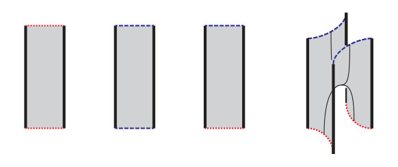 Figure 1
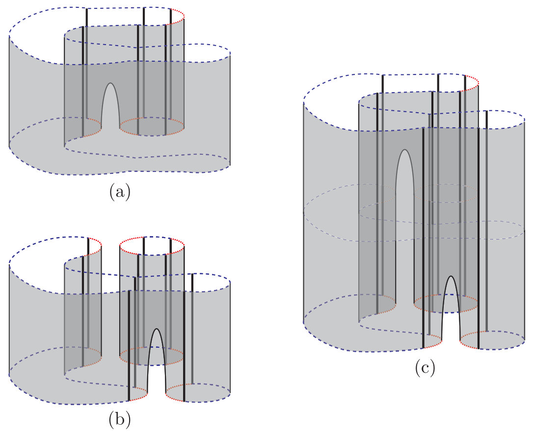 Figure 2
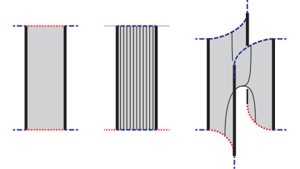 Figure 3
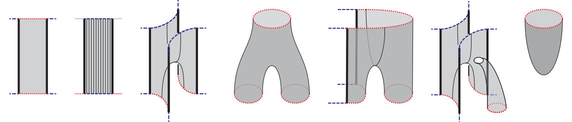 Figure 4
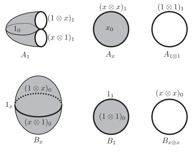 Figure 5
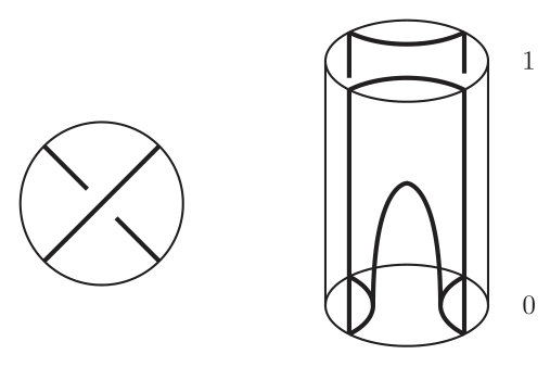 Figure 6
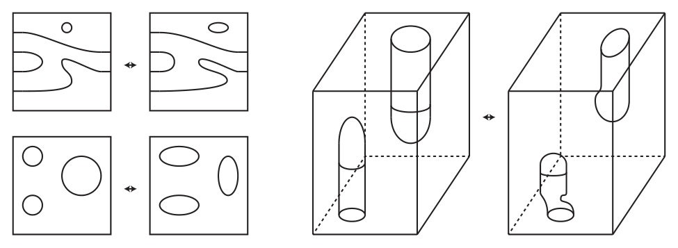 Figure 7
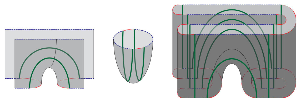 Figure 8
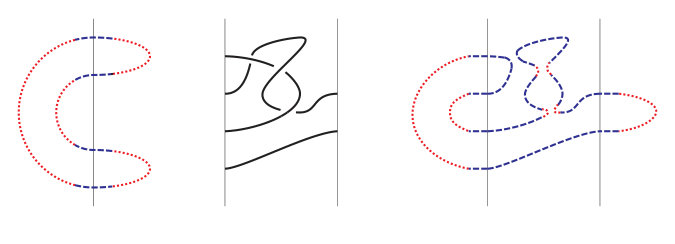 Figure 9
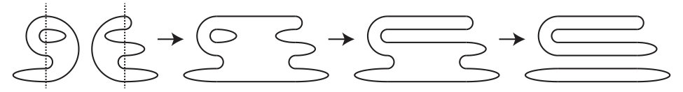 Figure 10
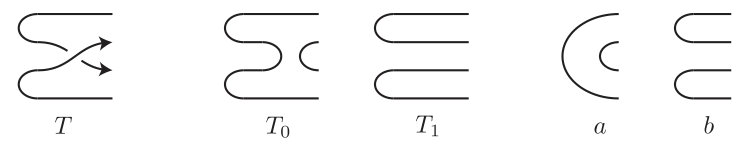 Figure 11
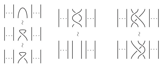 Figure 12
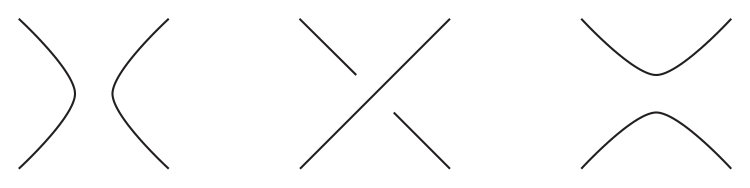 Figure 13
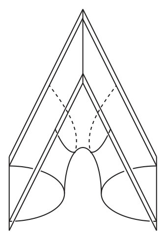 Figure 14
 Figure 15
 Figure 16
 Figure 17
 Figure 18
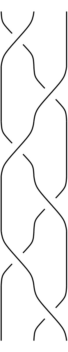 Figure 19
 Figure 20