Hirota bilinear equations for Painlev\'e transcendents
A.N.W. Hone, F. Zullo

TL;DR
This paper explores Hirota bilinear equations related to Painlevé transcendents, providing a general Taylor expansion framework for their tau-functions and connecting special cases like the first and second Painlevé equations and Weierstrass sigma function.
Contribution
It introduces a fourth-order Hirota bilinear equation for the tau-function of the fourth Painlevé equation and derives a general Taylor expansion applicable to various Painlevé and elliptic functions.
Findings
Derived a general Taylor expansion for Painlevé tau-functions.
Connected special cases to classical functions like Weierstrass sigma.
Provided a unified framework for analyzing Painlevé tau-functions.
Abstract
We present some observations on the tau-function for the fourth Painlev\'e equation. By considering a Hirota bilinear equation of order four for this tau-function, we describe the general form of the Taylor expansion around an arbitrary movable zero. The corresponding Taylor series for the tau-functions of the first and second Painlev\'e equations, as well as that for the Weierstrass sigma function, arise naturally as special cases, by setting certain parameters to zero.
Click any figure to enlarge with its caption.
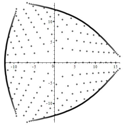 Figure 1
Peer Reviews
No public reviews on file for this paper yet. If you reviewed it on a platform where reviews are public (OpenReview, ICLR, NeurIPS, ICML), you can paste yours below so the community can read it here.
Videos
No videos yet. Explain this paper in a talk, walkthrough, or lecture? Add one.
A Hirota bilinear equation for Painlevé transcendents , and .
A.N.W. Hone, and F. Zullo SMSAS, University of Kent, Canterbury, U.K.Dipartimento di Ingegneria Meccanica e Aerospaziale, Università La Sapienza, Roma, Italy.
Abstract
We present some observations on the tau-function for the fourth Painlevé equation. By considering a Hirota bilinear equation of order four for this tau-function, we describe the general form of the Taylor expansion around an arbitrary movable zero. The corresponding Taylor series for the tau-functions of the first and second Painlevé equations, as well as that for the Weierstrass sigma function, arise naturally as special cases, by setting certain parameters to zero.
1 Introduction
The six Painlevé equations (denoted ) can be considered as nonlinear analogues of the classical functions: they admit a Hamiltonian representation [15], all of them (apart from ) possess Bäcklund transformations [2], and they each arise as a compatibility condition for an associated isomonodromy problem [13]. General solutions of Painlevé equations have asymptotics in terms of elliptic functions, which was originally obtained (for and ) by Boutroux [1]. It is also known that through a limiting procedure, usually called the coalescence cascade, it is possible to obtain all the equations just from equation (see e.g. [12]). Furthermore, the equations , and share the property that all their local solutions are meromorphic and possess a meromorphic continuation in the whole complex plane [11].
The Hamiltonian functions for - are polynomials in the canonically conjugate phase space variables , and are rational in the independent variable . Letting a prime denote differentiation with respect to , the Hamiltonian formulation allows each of the Painlevé equations to be formulated as a first order system,
[TABLE]
The functions themselves, as functions of the time , solve certain differential equations; these functions, defined by , where satisfy (1), are usually called “sigma functions” [13, 15]. Every solution of the Painlevé equation can be written in terms of the solution of a corresponding differential equation for , which is of second order and second degree. Moreover, the sigma function is given in terms of the logarithmic derivative of a tau-function. In some sense, one can view the sigma function or the tau-function as being more fundamental than the solution of the Painlevé equation, since in applications (such as in the theory of random matrices [7]) these are usually the main objects of interest.
In recent work [10] we have shown how the recursive formula for the coefficients in the Laurent series expansion of solutions of the first Painlevé equation can be considered as an extension of the analogous formula for the Weierstrass function. In addition, the recursive formulae for the Taylor expansion of the tau-function around one of its zeros lead to natural extensions of the expressions found by Weierstrass [18] for the elliptic sigma function (not to be confused with the sigma function of the Painlevé equations). The key to these recursive formulae was the use of a Hirota bilinear equation for the tau-function, amenable to the same method that was applied to the elliptic sigma function in [3].
The purpose of this short article is to derive recursive formulae for the expansion of the tau-function of the fourth Painlevé equation around a movable zero. Bilinear equations for tau-functions have been derived previously, either as a system of two equations relating two tau-functions [9], or as a symmetric system involving three tau-functions (see e.g. Theorem 3.5 in [14]). However, by starting from the equation for the sigma function , we can use a single Hirota bilinear equation of fourth order to obtain the Taylor series expansion of the tau-function around a zero. By exploiting the freedom in the definition of , we introduce additional parameters into the sigma function equation, and show how the corresponding series solutions for both and arise directly from the same bilinear equation as degenerate special cases, by setting suitable parameters to zero, while all of these series can be viewed as natural extensions of the elliptic case treated in [3].
In the next section we briefly review the Hamiltonian formulation of the fourth Painlevé equation and the corresponding sigma equation, before introducing a “shifted” sigma equation (given by (11) below), which is suitable for studying series expansions around movable poles, as well as the degeneration to , and elliptic functions. Section 3 is concerned with the properties of the tau-function for , the corresponding bilinear equation, and the presentation of the main result, namely the recursion for the Taylor coefficients (Theorem 3.2). The fourth section is devoted to a numerical application of the main result, using it to calculate approximations to the zeros of a particular tau-function for , and we end with some conclusions and suggestions for future work.
2 Hamiltonian and sigma equation for
The fourth Painlevé equation can be derived from the Hamiltonian function
[TABLE]
where and for are parameters. The corresponding Hamilton’s equations (1) are given explicitly by (hereafter a prime denotes a derivative with respect to )
[TABLE]
The ordinary differential equation of second order satisfied by arises by eliminating from (3), to yield
[TABLE]
where
[TABLE]
which (up to rescaling and ) is just the fourth Painlevé equation . By symmetry, upon eliminating from (3), it follows that satisfies
[TABLE]
with
[TABLE]
so that satisfies the same form (4) of as does, but for different values of the parameters .
There is a certain amount of redundancy in the choice of parameters used above. Although the parameter appears inessential, as (providing it is non-zero) it can always be removed by rescaling and , it will be needed in what follows. As for the three quantities , , the solutions of only depend on the differences , but the inclusion of the term in (2) shows that the sigma function
[TABLE]
also depends on the parameter
[TABLE]
Indeed, by taking derivatives of the Hamiltonian with respect to , it follows that the sigma function satisfies the following equation of second order and second degree:
[TABLE]
Moreover, and are given in terms of the solution of the latter equation by
[TABLE]
The freedom to permute shows that generically the same solution of (7) provides six different solutions of the equation (4), with different , ; this is one manifestation of the affine symmetry for [15], which can be seen more easily from its symmetric form [14].
Henceforth we regard the sigma equation (7) as the fundamental object of interest, and proceed to consider the behaviour of solutions near singularities. Since and are both meromorphic for all (see e.g. [11] or [17]), it follows from (2) that is also a globally meromorphic function, and it is straightforward to see that its only possible singularities are movable simple poles with a local Laurent expansion of the form
[TABLE]
where both the pole position and the quantity (resonance parameter) are arbitrary. For fixed values of the coefficients and , any solution of the second order equation (7) is completely specified by a particular choice of the two values in (9), which is then determined on the whole complex plane by analytic continuation.
In order to understand how the solution of (7) depends on the parameters , it is convenient to shift
[TABLE]
which leads to an equation of the form
[TABLE]
where
[TABLE]
and for , the dependent variable is given by
[TABLE]
with the parameters being polynomials in and the . Having fixed the pole to lie at , and shifted away the parameter , the function satisfying (11) depends only on the 5 parameters , while depends on also.
Lemma 2.1**.**
For , via translations of the form (10), there is a one-to-one correspondence between solutions of (7) with a pole at some , and functions
[TABLE]
with a pole at , where is the solution of (11) specified by the local Laurent expansion
[TABLE]
Remark 2.2**.**
The above result applies to any solution of (7) with at least one pole; in particular, this excludes certain trivial solutions which are linear in . If we scale (4) so that , then all solutions of which are transcendental, meaning that they are neither rational nor can be reduced to solutions of a Riccati equation, have infinitely many simple poles with residue and infinitely many with residue [8]. The formula (8) shows that (for ) has a pole with residue at places where has a simple pole, and does not depend on the parameter , so its behaviour near such a pole is completely determined by a function specified as above. Poles of with residue correspond to places where has a zero with ; the behaviour at such poles can also be determined by using the well known observation of Okamoto [15] that when every solution of (4) can be written as the difference of two Hamiltonians, i.e.
[TABLE]
where satisfies (7) but with suitably shifted parameters.
For future reference, we record the equation of third order that results by taking the derivative of (11) and removing a factor of , that is
[TABLE]
Clearly the parameter in (11) is a first integral for the above equation.
We now consider the degenerate case , which is no longer related to .
Proposition 2.3**.**
If and , then
[TABLE]
satisfies the equation in the form
[TABLE]
where
[TABLE]
Thus
[TABLE]
satisfies the second Painlevé equation in the form
[TABLE]
and conversely is given in terms of and its first derivative by
[TABLE]
Proof.
If , then (11) reduces to the sigma equation for , provided that . Upon multiplying (14) by and subtracting off half of (11), the terms involving are eliminated, and what remains is the equation (16) for , which is referred to as in [12]. Every solution of (16) gives a solution of (18), and vice-versa, according to the formulae (17) and (19). ∎
Remark 2.4**.**
The relations (17) and (19) can be rewritten as
[TABLE]
which is the Hamiltonian formulation of found in [15]. The standard version of (16), or that of (18), has . However, the situation for , is completely analogous to that in Lemma 2.1: we can use expansions around for , of the form, (13) to obtain local Laurent expansions for the standard version of (or ) around a pole in an arbitrary position .
When , then a further degeneration occurs.
Proposition 2.5**.**
If and , then
[TABLE]
satisfies the first Painlevé equation in the form
[TABLE]
while if , then the general solution of (11) is given in terms of the Weierstrass zeta function with invariants by
[TABLE]
for arbitrary, so is an elliptic function of .
Proof.
Up to replacing , this coincides with the case considered in [10]. ∎
3 Tau-function and bilinear equation
For the sigma equation in the form (11), the tau-function is defined by
[TABLE]
Since is meromorphic, with its only singularities being simple poles with residue , the above formula implies that is holomorphic, but is only defined up to overall scaling for an arbitrary non-zero constant . By substituting (22) into (11), an equation of third order which is homogeneous of degree four in results, that is
[TABLE]
Taylor expansions of (23) around a movable zero, which correspond to a movable simple pole in (11), take the form
[TABLE]
where (the position of the zero) and are arbitrary, while all subsequent coefficients are determined uniquely in terms of these three parameters. By considering gauge transformations of the form
[TABLE]
the initial coefficient can be set to 1, and can be set to [math]; in that case one can check that the next coefficient is also [math]. The overall effect of the transformation (24) is to send
[TABLE]
which results in changing the parameters in (11) and (23). However, this change does not affect the form of the equation, and thus we obtain an alternative version of Lemma 2.1, reformulated in terms of the tau-function.
Lemma 3.1**.**
For , via translations of the form (10), there is a one-to-one correspondence between solutions of (7) with a pole at some , and functions
[TABLE]
with a pole at , where is the solution of (23) specified by the local Taylor expansion
[TABLE]
The degree four equation (23) is somewhat awkward for computing the coefficients in the local expansion
[TABLE]
around a zero at . It is much more convenient to take the derivative of (23), so that after removing an overall factor one finds the bilinear (degree two) equation
[TABLE]
which has been written concisely in terms of the Hirota derivative defined by
[TABLE]
The equation (27) also follows immediately by making the substitution (22) in (14). The quantity in (23) also corresponds to a first integral of (27).
In order to describe the expansion of the tau-function around a zero, we use the bilinear equation (27), and note that the action of the Hirota operators and on monomials is given by
[TABLE]
where the multipliers appearing on the right-hand side are
[TABLE]
The resulting recursion relation leaves the coefficients and undetermined. The freedom to chose in (27) corresponds to the value of the first integral , so in order to match the term at order arising from (23), the correct value of must be inserted in the recursion. Before stating the result, it is convenient to define the shifted multipliers
[TABLE]
Theorem 3.2**.**
The coefficients in the expansion (26) obey the recursion
[TABLE]
To obtain the expansion in the form (25), the free coefficients must be fixed as
[TABLE]
With the latter choice, each coefficient is a weighted homogeneous polynomial of total degree in with weights respectively, so that
[TABLE]
where for all .
This above result extends the analogous recursion for the Taylor series coefficients of the Weierstrass sigma function [3] and for the tau-function of the first Painlevé equation [10]. We record the first few polynomials here:
[TABLE]
Computer calculations up to suggest that, after suitable scaling of the variables , these polynomials have integer coefficients. The form of the expression (30) implies that the Taylor series solution of (23) with leading order (25) can be written as a multiple sum
[TABLE]
where .
Conjecture 3.3**.**
The series (31) has
[TABLE]
Remark 3.4**.**
In the case , Weierstrass [18] considered the series for the elliptic sigma function in the form (31), and Onishi proved that for all [16], while in [10] we already found considerable numerical evidence to suggest that .
The tau-function transforms in a very specific way when it is expanded around another zero, at a location .
Proposition 3.5**.**
Let denote the solution of (23) having the Taylor expansion (25) around , and suppose that this function also vanishes at . Then
[TABLE]
where
[TABLE]
[TABLE]
Proof.
Upon replacing in (23), and introducing
[TABLE]
we see that satisfies an equation of the general form (7), and has a pole at because . If we now set
[TABLE]
with given by the expression in (33), then for any choice of , satisfies an equation of the canonical form (11), but with different coefficients . Now we further require that
[TABLE]
where has the Taylor expansion (25) around . By integrating both sides of (34) and exponentiating, we see that
[TABLE]
for some . By performing a Taylor expansion on each side of the above relation up to terms of order , we obtain the expressions for and as in (33), as well as the equation
[TABLE]
The latter formula can be seen to be consistent with the previous expression for by setting in (23). Hence satisfies the same equation (23) but with parameters found from the equation corresponding equation (11) for . ∎
Remark 3.6**.**
The expression (32) is a generalization of the classical formula for transformation of the Weierstrass sigma function under shifting by a period (see e.g. in [19]).
4 Numerical example: poles in
The numerical evaluation of Painlevé transcendents and the structure of their pole fields is a very active research area (see e.g. [4]-[6] and references therein). The recursion relation in Theorem 3.2 is extremely convenient for computing numerical approximations to the tau-function close to the origin, by truncating the Taylor series for . The roots of the polynomials obtained by truncation provide approximations to the zeros of the tau-function lying near to , or equivalently the positions of the poles of the sigma equation.
As an example, we consider the case of parameters
[TABLE]
for which the function is such that
[TABLE]
satisfies the equation in the canonical form
[TABLE]
with parameter , while from (17) we have that
[TABLE]
satisfies in the form
[TABLE]
For the parameter values (35), the equation (11) admits a trivial solution const, giving , but we have neglected such solutions here, by considering the generic situation where has poles (cf. Lemma 2.1). (In fact, setting in (19) yields a Riccati equation, corresponding to the special case that (38) is solved in Airy functions.) The tau-function given by the Taylor series defined in Theorem 3.2 is such that the expansion (31) takes the special form
[TABLE]
which is invariant under the order 3 symmetry
[TABLE]
Hence the zeros of have the same symmetry: if is a zero of , then so are and . These zeros of are the simple poles of , and the double poles of , i.e. the particular solution of (37) defined by (36). Similarly, the associated function that satisfies the case (38) of has simple poles with residue at these same positions, as well as simple poles with residue at the places where vanishes, all of them symmetrically placed on triangles centred at [math].
For illustration, in Figure 1 we have plotted the approximate positions of some of the zeros of (or the equivalently the poles of and ). To begin with, the first 201 non-zero terms of the series (39) were found. The first few coefficients have prime factorizations
[TABLE]
and it appears to be the case that
[TABLE]
To prove either of these two statements seems not to be simple. However from the bilinear equation (27) it follows that the coefficients are determined by the quadratic recurrence
[TABLE]
subject to the initial conditions , and . The values of and are defined by the action of the Hirota operators and on polynomials (see before Theorem 3.2).
Given these coefficients, we took the polynomial
[TABLE]
and calculated its roots numerically in order to produce the figure. By comparing the values of the roots with those of the successive approximations , , , , etc. we were able to confirm that the values of the zeros closest to [math] were converging to a high degree of accuracy. For instance, the non-zero roots closest to the origin lie at , and the next closest roots are at , where
[TABLE]
to 20 decimal places. The largest roots of the polynomial, which can be seen to coalesce on the boundary of the figure, are numerical artefacts; they do not provide good approximations to the zeros of the tau-function.
Remark 4.1**.**
Due to the homogeneity of the parameters , , all of the tau-functions admit the symmetry (40).
Remark 4.2**.**
Non-polynomial rational solutions of the sigma equation are also included in the formulation of Lemma 2.1. For example, for the parameter values
[TABLE]
the equation (11) has the rational solution
[TABLE]
corresponding to the tau-function
[TABLE]
which illustrates the symmetry (40) explicitly. This corresponds to
[TABLE]
which are rational solutions of the equation (16) and the equation (18), respectively, with , , .
5 Conclusions
Our analysis shows that the “shifted” sigma equation for , given by (11), is a fundamental object which contains not only the general solution of , but also that of , , and the Weierstrass function. Although the connection between Painlevé transcendents and elliptic functions has a long history at the level of asymptotic expansions [1], the results presented here show that from the viewpoint of the sigma function the Painlevé transcendents are multi-parameter extensions of elliptic functions. Furthermore, although there is a coalescence cascade , this requires taking asymptotic limits of both the dependent and independent variables [12], whereas at the level of the solution of (11) one has , with the inclusion denoting that a parameter has been set to zero. It would be interesting to see if this approach can be extended to the sigma function of , in which case all the other Painlevé equations would be included as special cases.
In future work we propose to consider Mittag-Leffler expansions of the solutions of (11), and the asymptotic behaviour of the coefficients in Laurent expansions for the solutions of the sigma equation, as well as the corresponding Painlevé equations. It would also be good to obtain precise a priori bounds on the growth of the polynomials appearing in Theorem 3.2, as this would yield an independent proof that the tau-function is holomorphic (hence providing yet another proof of the Painlevé property for , and ; cf. [17]). The arithmetic properties of the coefficients in (31) are also worthy of further study.
Acknowledgements: ANWH is supported by EPSRC fellowship EP/M004333/1. FZ wishes to acknowledge the financial support of the GNFM-INdAM, SISSA (Trieste) and CRM Ennio de Giorgi (Pisa) for participation in the workshop “Asymptotic and computational aspects of complex differential equations,” held in Pisa from - February 2017. Both authors are grateful to the organisers of the LMS-EPSRC Durham Symposium on Geometric and Algebraic Aspects of Integrability, July - August 2016, which gave us an opportunity to renew our collaboration.
The reference list from the paper itself. Each links out to its DOI / PubMed record.
- 1[1] Boutroux P.: Recherches sur les transcendantes de M. Painlevé et l’étude asymptotique des équations différentielles du second ordre, Ann. École Norm. 30, 265-375, 1913.
- 2[2] Clarkson P.A.: Painlevé Equations - nonlinear special functions, in Orthogonal Polynomials and Special Functions: Computation and Application, F. Márcellan and W. van Assche Ed., Lecture Notes in Mathematics, 1883, Springer-Verlag, Berlin, pp 331-411, 2006.
- 3[3] J.C. Eilbeck and V.Z. Enolskii, Bilinear operators and the power series for the Weierstrass σ 𝜎 \sigma function, J. Phys. A: Math. Gen. 33 , 791–794, 2000.
- 4[4] B. Fornberg and J. A. Reeger: Painlevé IV: A numerical study of the fundamental domain and beyond. Physica D , 280-281 , 1-13, 2014.
- 5[5] B. Fornberg and J. A. C. Weideman: A computational exploration of the second Painlevé equation. Found. Comput. Math. , 14 , 985–1016, 2014.
- 6[6] B. Fornberg and J. A. Reeger: Painlevé IV with both parameters zero: A numerical study. Stud. Appl. Math. , 130 , 108–133, 2013.
- 7[7] Forrester, P.J., Witte, N.S., Application of the tau-function theory of Painlevé equations to random matrices: PIV, PII and the GUE, Communications in Mathematical Physics , 219 , 357–398, 2001.
- 8[8] Gromak V.I., Laine I., Shimomura S.: Painlevé Differential Equations in the Complex Plane, Walter de Gruyter Studies in Mathematics 28, Berlin, New York, 2002.