TL;DR
This paper introduces a large-scale label propagation method for low-shot image classification, leveraging similarity graphs over hundreds of millions of images to achieve state-of-the-art accuracy.
Contribution
It demonstrates that scaling label propagation to massive datasets significantly improves low-shot learning performance.
Findings
Scaling label propagation to hundreds of millions of images yields state-of-the-art accuracy.
Large-scale similarity graphs effectively support label propagation in low-shot learning.
The approach outperforms traditional fine-tuning methods in low-data regimes.
Abstract
This paper considers the problem of inferring image labels from images when only a few annotated examples are available at training time. This setup is often referred to as low-shot learning, where a standard approach is to re-train the last few layers of a convolutional neural network learned on separate classes for which training examples are abundant. We consider a semi-supervised setting based on a large collection of images to support label propagation. This is possible by leveraging the recent advances on large-scale similarity graph construction. We show that despite its conceptual simplicity, scaling label propagation up to hundred millions of images leads to state of the art accuracy in the low-shot learning regime.
Click any figure to enlarge with its caption.
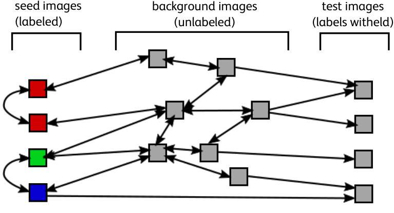 Figure 1
 Figure 2
 Figure 3
 Figure 4
 Figure 5
 Figure 6
 Figure 7
 Figure 8
 Figure 9
 Figure 10
 Figure 11
 Figure 12
 Figure 13
 Figure 14
 Figure 15
 Figure 16
 Figure 17
 Figure 18
 Figure 19
 Figure 20
 Figure 21
 Figure 22
 Figure 23
 Figure 24
 Figure 25
 Figure 26
 Figure 27
 Figure 28
 Figure 29
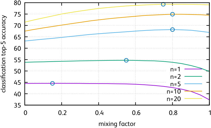 Figure 30
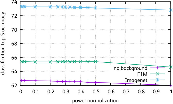 Figure 31
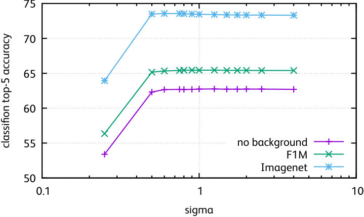 Figure 32
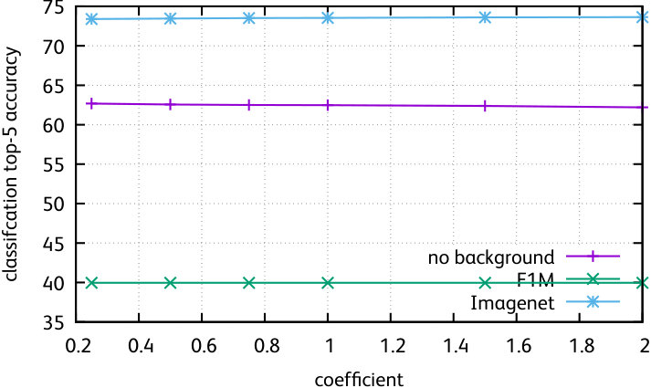 Figure 33
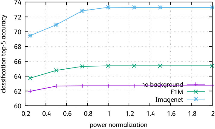 Figure 34
| out-of-domain diffusion | in-domain | logistic | combined | best reported | |||||
|---|---|---|---|---|---|---|---|---|---|
| none | F1M | F10M | F100M | (Imagenet) | regression | +F10M | + F100M | results [bharath2017low] | |
| 39.40.85 | 43.90.96 | 46.31.28 | 47.61.09 | 57.71.28 | 42.61.31 | 46.51.23 | 47.91.18 | 45.1 | |
| 47.80.94 | 52.71.14 | 55.21.21 | 57.01.05 | 66.91.06 | 54.41.29 | 57.51.34 | 58.41.29 | 58.8 | |
| 56.80.73 | 62.20.44 | 64.60.57 | 66.30.68 | 73.80.29 | 71.40.54 | 71.90.55 | 72.30.58 | 72.7 | |
| 64.90.28 | 68.00.33 | 69.90.47 | 71.70.54 | 77.60.23 | 78.60.27 | 78.70.21 | 79.20.14 | 79.1 | |
| 71.40.26 | 72.70.40 | 74.10.38 | 75.30.29 | 80.00.21 | 82.90.20 | 83.00.15 | 83.20.22 | 82.6 | |
Peer Reviews
No public reviews on file for this paper yet. If you reviewed it on a platform where reviews are public (OpenReview, ICLR, NeurIPS, ICML), you can paste yours below so the community can read it here.
Code & Models
Videos
No videos yet. Explain this paper in a talk, walkthrough, or lecture? Add one.
\definecolor
darkgreenRGB0, 140, 0
Supplementary material for:
Low-shot learning with large-scale diffusion
Matthijs Douze, Arthur Szlam, Bharath Hariharan , Hervé Jégou
Facebook AI Research
*Cornell University This work was carried out while B. Hariharan was post-doc at FAIR.
\appendix
We present several additional results and details to complement the paper. Section 1 reports another evaluation protocol, which restricts the evaluation to novel classes. Sections 2 and 3 are parametric evaluations. Section 4 gives some details about the graph computation.
1 Evaluation results on novel classes
In the main paper, we evaluated the search performance on all the test images from group 2. The performance restricted to only the novel classes is also reported in prior work [bharath2017low] using a combination of classifiers. Table 1 shows the results in this setting.
As to be expected, the results reported in these tables are inferior to those obtained in the setup where all test images are classified. This is because the novel classes are harder to classify than the base classes. Otherwise the ordering of the methods is preserved and the conclusions identical. The diffusion is effective in the low-shot regime and is, by itself, better than the state of the art by a large margin when only one example is available. The combination with late fusion significantly outperforms the state of the art, even in the out-of-domain setup.
2 Details of the parametric evaluation
In the paper we reported results for the edge weighting and graph normalization with the best parameter setting. Here, we report results for all parameters111Note that our parametric experiments use the set of baseline image descriptors used in the arXiv version of the paper by Barath \etal [bharath2017low], and the figure compares all methods using those underlying features. Therefore the results are not directly comparable with the rest of the paper. . We evaluate the following edge weightings (Figure 2, first row):
- •
Gaussian weighting. The edge weight is with the distance between the edge nodes. Note that corresponds to a constant weighting;
- •
Weighting based on the “meaningful neighbors” proposal [ODL07]. It relies on an exponential fit of neighbor distances. For a given graph node, for the neighbor of its list of results, the weight is , where is the distance, remapped linearly to so that the first neighbor has and the th neighbor has . We vary parameter in the plot.
We also report results for different normalizations of the matrix . In Figure 2 (second row), we compare:
- •
The non-linear normalization, all elements of are raised to a power . We vary the parameter , and corresponds to the identity transform;
- •
We classify all images in a graph with a logistic regression classifier. We use the predicted frequency of each class over the whole graph, and raise it to some power (the parameter) to reduce or increase its peakiness. This choice is inspired by the Markov Clustering Algorithm [EDO2002]. This gives a normalization factor that we enforce for each column of , instead of the default uniform distribution.
The conclusion of these experiments is that these variants do not improve over constant weights and a standard diffusion, most of them having a neutral effect. Therefore, we conclude that the diffusion process mostly depends on the topology of the graph.
3 Late fusion weights
Let denote by and the distributions over classes returned by the two classifiers for image . We fuse the loglikehood by a weighted average, which amounts to retrieving the top-5 class prediction as those maximizing
[TABLE]
where is the optimal mixing coefficient for seed points, as found by cross-validation.
Figure 3 shows these optimal mixing factors. Since the logistic regression is better at classifying with many training examples, the parameter increases with .
4 Computation of the blocks
As stated in the paper, we need to compute the 4 blocks of the matrix :
[TABLE]
where, usually, . Each block requires to perform a -nearest neighbor search. We employ the Faiss library222http://github.com/facebookresearch/faiss optimized for this task [johnson2017billion], and use it as follows:
- •
: we use a Faiss index referred to as “IVFFlat”. The accuracy-speed compromise is controlled by a parameter giving the number of inverted lists visited at search time. We adopted a relatively high probe setting (256) to guarantee that most of the actual neighbors are retrieved. With the recommended settings of Faiss, the complexity of one search is proportional to , so the total complexity is . This is super-linear with respect to , but it is still relatively efficient (see our timings) and performed off-line;
- •
: we re-use the same index to do similarity search operations, this time using only ;
- •
: we need to index on the seed image descriptors. We found that in practice, constructing an index on these images is at best 1.4 faster than brute-force search. Therefore, we use brute-force search in this case, which if of order ;
- •
: it has a negligible complexity.
The fusion of the result lists and to get results per row of is done in a single pass and in a negligible amount of time. Therefore the dominant complexity is . A typical breakdown of the timings for F100M is (in seconds):
[TABLE]
For we decompose the timing into: loading of the precomputed IVFFlat index (and moving it to GPU if appropriate) and the actual computation of the neighbors.
