Initial state qqg correlations as a background for the Chiral Magnetic Effect in collision of small systems
Alex Kovner, Michael Lublinsky, Vladimir Skokov

TL;DR
This paper calculates initial state three-particle correlations in proton-nucleus collisions within the Color Glass Condensate framework to understand background signals for the Chiral Magnetic Effect, revealing rapidity-dependent effects that could influence experimental observations.
Contribution
It provides the first calculation of three-particle correlations involving two quarks and one gluon in the initial state, highlighting rapidity dependence and potential impact on CME background understanding.
Findings
Two distinct contributions to correlations: rapidity-independent and rapidity-dependent.
Rapidity-dependent contribution leads to negative same-charge correlations at large rapidity separation.
Initial state correlations may partially explain experimental CME signals.
Abstract
Motivated by understanding the background to Chiral Magnetic Effect in proton-nucleus collisions from first principles, we compute the three particle correlation in the projectile wave function. We extract the correlations between two quarks and one gluon in the framework of the Color Glass Condensate. This is related to the same-charge correlation of the conventional observable for the Chiral Magnetic Effect. We show that there are two different contributions to this correlation function. One contribution is rapidity-independent and as such can be identified with the pedestal; while the other displays rather strong rapidity dependence. The pedestal contribution and the rapidity-dependent contribution at large rapidity separation between the two quarks result in the negative same charge correlations, while at small rapidity separation the second contribution changes sign. We argue that…
Click any figure to enlarge with its caption.
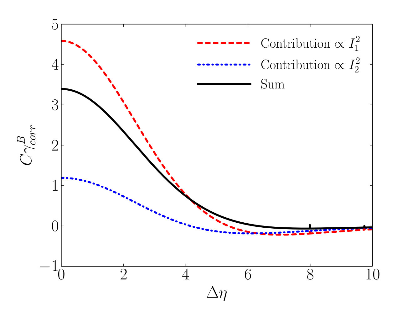 Figure 1
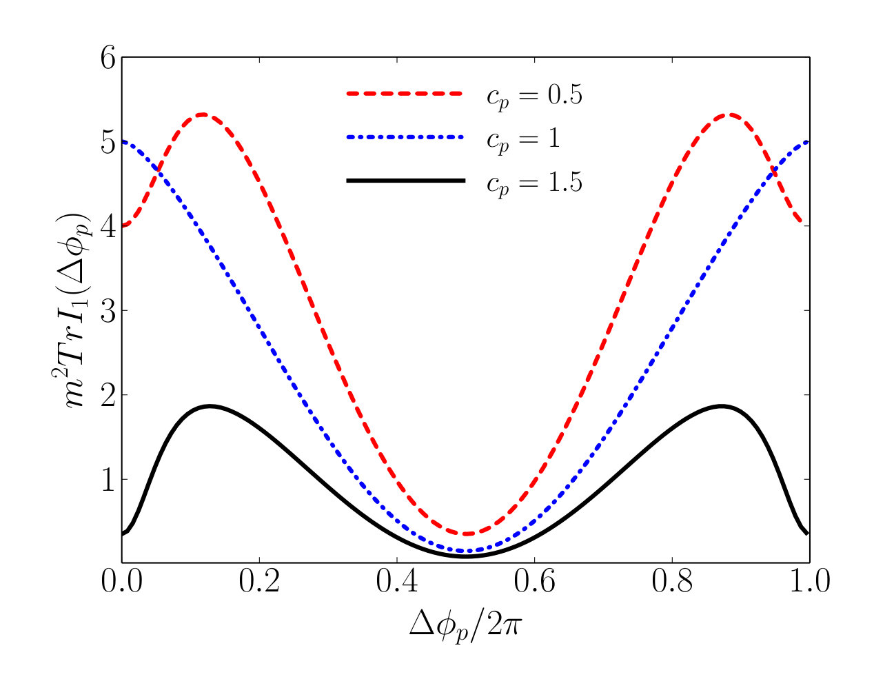 Figure 2
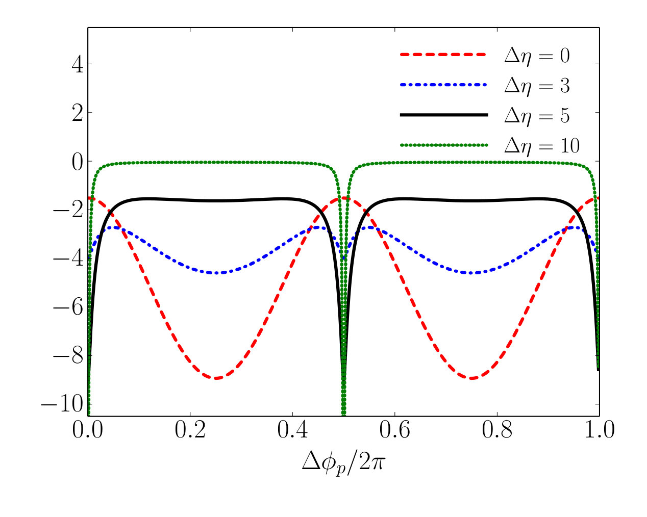 Figure 3
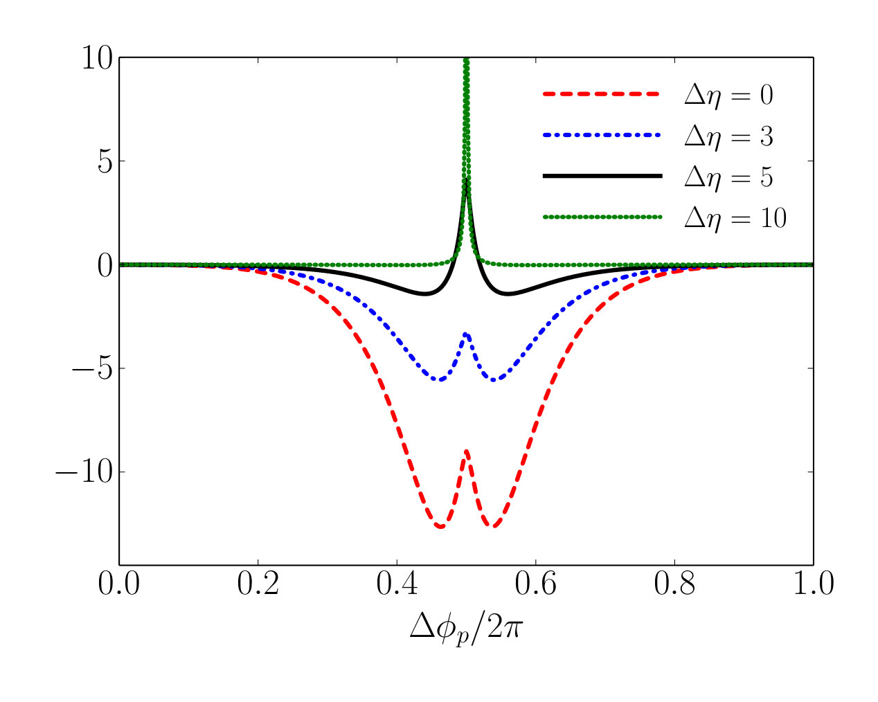 Figure 4
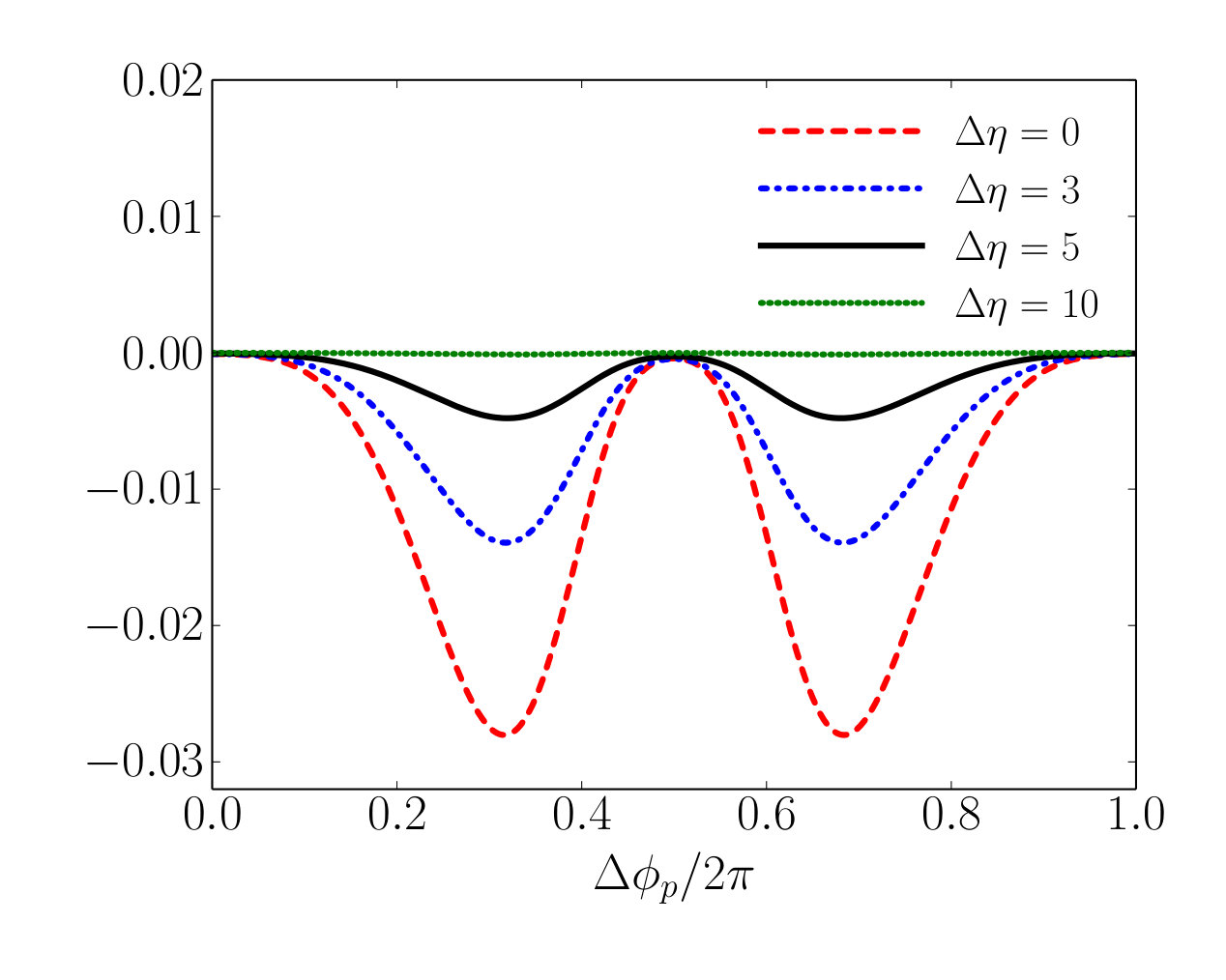 Figure 5
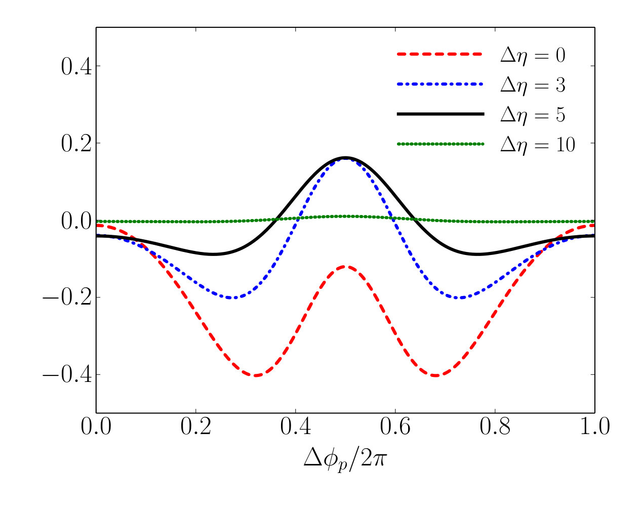 Figure 6
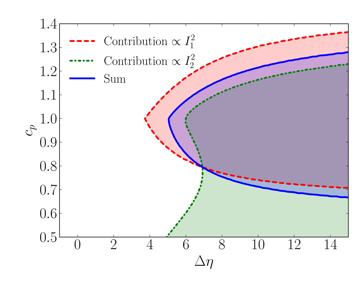 Figure 7
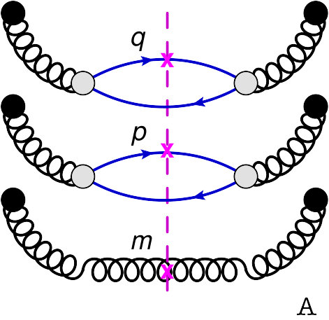 Figure 8
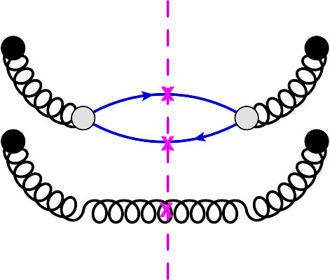 Figure 9
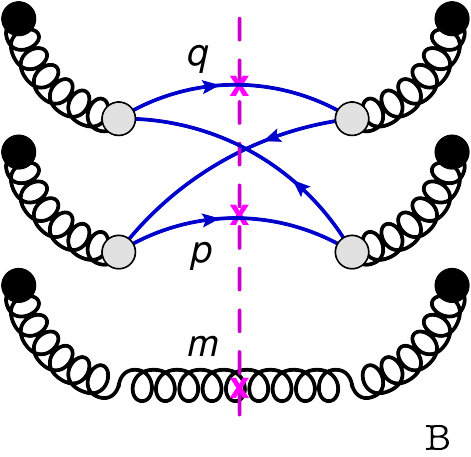 Figure 10
Peer Reviews
No public reviews on file for this paper yet. If you reviewed it on a platform where reviews are public (OpenReview, ICLR, NeurIPS, ICML), you can paste yours below so the community can read it here.
Videos
No videos yet. Explain this paper in a talk, walkthrough, or lecture? Add one.
Initial state correlations as a background for the Chiral Magnetic Effect in collision of small systems.
Alex Kovner
Physics Department, University of Connecticut, 2152 Hillside Road, Storrs, CT 06269, USA
Departamento de Física, Universidad Técnica Federico Santa María, Avda. España 1680, Casilla 110-V, Valparaiso, Chile
Michael Lublinsky
Physics Department, Ben-Gurion University of the Negev, Beer Sheva 84105, Israel
Vladimir Skokov
RIKEN/BNL, Brookhaven National Laboratory, Upton, NY 11973
Abstract
Motivated by understanding the background to Chiral Magnetic Effect in proton-nucleus collisions from first principles, we compute the three particle correlation in the projectile wave function. We extract the correlations between two quarks and one gluon in the framework of the Color Glass Condensate. This is related to the same-charge correlation of the conventional observable for the Chiral Magnetic Effect. We show that there are two different contributions to this correlation function. One contribution is rapidity-independent and as such can be identified with the pedestal; while the other displays rather strong rapidity dependence. The pedestal contribution and the rapidity-dependent contribution at large rapidity separation between the two quarks result in the negative same charge correlations, while at small rapidity separation the second contribution changes sign. We argue that the computed initial state correlations might be partially responsible for the experimentally observed signal in proton-nucleus collisions.
††preprint: RBRC 1242
I Introduction
Topological fluctuations in the early time Glasma state Mace et al. (2016, 2017) or thermal sphaleron transitions Arnold and McLerran (1987); Moore and Tassler (2011) during later stages of heavy-ion collisions may lead to the Chiral Magnetic Effect (CME) Kharzeev et al. (2008), the generation of the electromagnetic current along the magnetic field Skokov et al. (2009); Bzdak and Skokov (2012); McLerran and Skokov (2014). Experimentally, the associated charge separation can be measured by three particle angular average Voloshin (2004), , where is the azimuthal angle of a trigger particle defining the reaction plane and are azimuthal angles of associate particles carrying electric charge. The averaging is usually taken over a range of transverse momenta of the charged particles. The observable is also often considered as a function of relative rapidity separation between the charge particles and the multiplicity/centrality of the collision. The charge of the particles and can be either same or opposite. For more information about the experimental measurements, see Ref. Voloshin (2004); Abelev et al. (2009, 2010); Khachatryan et al. (2017); Skokov et al. (2016); Tribedy (2017).
The CME prediction for the observable can be understood as follows. In the presence of the strong magnetic field, , and initial axial charge , the CME builds an electric current along the magnetic field Kharzeev et al. (2008), which in non-central heavy-ion collisions points in the out-of-plane directions, see Refs. Skokov et al. (2009); Bzdak and Skokov (2012). The current results in the transport of the charges and subsequent formation of a dipole moment in the charge distribution, which can be described by
[TABLE]
where is the reaction plane angle (neglecting the fluctuations, the magnetic field is perpendicular to the reaction plane), is the directed flow, is the elliptic flow and denotes the charge of the particles. The parameters describe the formation of the electric dipole . The sign of fluctuates on event by event basis rendering . Nevertheless, the parity-even fluctuations, , can still be measured in experiment. The observable suppresses the background Voloshin (2004) and is approximately equals to the fluctuations, that is
[TABLE]
From this expression one can draw conclusions on the CME predictions for . For the same charges , and thus one expects ; for opposite charges , and thus . Additionally, if the backgrounds effects are negligible, the same-charge correlator should be opposite in sign but equal in magnitude to opposite-sign correlator.
In collision with heavy-ions, the first measurement of were performed at RHIC Abelev et al. (2009, 2010); it was observed that opposite-charge correlations were very close to zero or even negative, while the same-charge were negative and larger in the amplitude. The observation of close to zero opposite-charge correlations was not immediately consistent with CME, as it was predicted to have the same amplitude as same-charge. However, the observable might be potentially contaminated by large charge-independent backgrounds, that shift the values of both the same-charge and opposite-charge correlations.
In order to test CME, a few other measurements and observables were explored, for details see Ref. Kharzeev et al. (2016); Skokov et al. (2016). Nevertheless, the status of the CME in heavy-ion collisions remains inconclusive due to background correlations that may be responsible for the entirety of the observed signal Schlichting and Pratt (2011); Pratt et al. (2011); Bzdak et al. (2011, 2013).
Recently, the CMS collaboration performed measurements of the three particle correlations in proton-nucleus collisions Khachatryan et al. (2017) at = 5 TeV. The CME predicts virtually absent signal in p-A collisions due to small values of the magnetic field and its decorrelation with the event plane. However, it was observed that the differences between the same and opposite sign correlations, as functions of multiplicity and rapidity gap between the two charged particles, are of a similar magnitude in proton-nucleus and nucleus-nucleus collisions at the same multiplicities. This does not necessarily pose an immediate challenge to the CME interpretation of the charge dependent azimuthal correlations in heavy ion collisions, as the results coincide only in peripheral bins of Pb-Pb collisions, where the background effects are expected to play a dominant role Tribedy (2017).
Nevertheless, the CMS measurements make it clear that without microscopic understanding of the background contributions to the observable , any interpretation of the data will be unsatisfactory. Motivated by the data of the CMS collaboration, in this paper, we address one of the possible sources of this background; we concentrate on the same-charge correlations, which usually fall outside the scope of the conventional background models Schlichting and Pratt (2011); Hirono et al. (2014) except for the global transverse momentum conservation. We work in the framework of the Color Glass Condensate; which was successful in predicting the “ridge” correlations and is often utilized to address the systematics of the azimuthal anisotropy in the initial state, see Refs. Dumitru et al. (2011); Kovner and Lublinsky (2011, 2013); Kovchegov and Wertepny (2013); Dusling and Venugopalan (2012, 2013); Dumitru et al. (2015a); Skokov (2015); McLerran and Skokov (2017); Lappi (2015); Schenke et al. (2015); Dumitru et al. (2015b); Altinoluk et al. (2015); Lappi et al. (2016); McLerran and Skokov (2016); Schlichting and Tribedy (2016); Dusling et al. (2017); Gotsman and Levin (2017).
As was shown in Ref. Altinoluk et al. (2015) the Bose-Einstein enhancement (BSE) of soft gluons in the projectile provides the physical interpretation of the glasma-graph calculation of the “ridge” correlations. In a follow up paper the authors of Ref. Altinoluk et al. (2017) also explored the consequences of quark’s Pauli blocking in the projectile wave function. Mindful of these studies, we consider the observable and explore possible nontrivial contribution to this observable, and therefore the CME background stemming from the quantum correlations in the initial state. In practice, we consider the angular average defined as a projectile average where and are the transverse momenta of two same-charge/same-flavor quarks in the light cone wave-function of the projectile, and is the transverse momentum of the gluon. We will demonstrate that there are two distinct contributions to this quantity: the pedestal, the rapidity-independent contribution, with a negative , and the rapidity-dependent and sign changing contribution originating from Pauli blocking.
The paper is organized as follows. In Sec. II we briefly review the relevant results of Ref. Altinoluk et al. (2017) for quark-quark correlations, originating from two quark-antiquark pairs in the wave function. In Sec. III we extend this calculation to include three particle correlations, computing contribution of an additional gluon thus bringing up the relevant Fock state component to 5 particles. In this paper we limit ourselves to the calculation of correlations in the wave function of the incoming hadron, and do not attempt to calculate three particle production, which we leave for future work. Nevertheless, as demonstrated in Altinoluk et al. (2015, 2017) such initial state correlations within the CGC approach have a direct effect on production of particles, and thus can serve as a basis for qualitative understanding of the effect. In Sec. IV we discuss and summarize our findings.
II Preliminaries: Quark contribution to the projectile wave-function
Let and denote quark creation and annihilation operators, while and are those of the antiquark. Additionally for gluons, we introduce and .
First we formulate, two particle, quark-antiquark, content of the light-cone wave function. This will allow us to introduce the notation we use when considering a more complicated case of two quark-two antiquark and gluon. In perturbative calculations, the quarks and antiquarks appear in the light-cone wave function of a valence charge via soft-gluon splitting or instantaneous interaction, see details in Ref. Altinoluk et al. (2017), Appendix A and the review Kogut and Soper (1970); Bjorken et al. (1971); Brodsky et al. (1998). The quark-antiquark component of the light cone wave function of a “dressed” color charge density is given by111The state to this order in perturbation theory contains one-gluon and two-gluon components. We do not indicate those explicitly, as they do not contribute to correlated quark-gluon production. These contributions were studied, e.g. in Refs. Altinoluk et al. (2015).
[TABLE]
where denotes a valence state characterised by a distribution of charge densities of valence (fast) partons. The subscript “2” in counts the perturbative order in the Yang-Mills coupling denoted as . is a constant ensuring the correct normalisation of the dressed state, are fundamental color indices, and stand for the spinor indices. The value of is irrelevant for the problem at hand. We define the longitudinal momentum fraction as
[TABLE]
with the momentum of the parent gluon that splits into a quark and an antiquark. The splitting amplitude is given by
[TABLE]
where are the generators of in the fundamental representation. Here,
[TABLE]
with
[TABLE]
and
[TABLE]
Thus,
[TABLE]
where
[TABLE]
The term comes from the instantaneous interaction, while from the soft gluon splitting.
However, is not the state we are interested in, as it provides information about quark-antiquark content of the light cone wave function only. To probe quark-quark-gluon correlations we have to consider the two quark–two antiquark and gluon component of the dressed state, that is the state with 5 particles. We will adopt the same strategy as was used in the glasma graph calculation. That is, we focus on terms enhanced by the charge density in the wave-function; similar approach was also used in Ref. Kovchegov and Wertepny (2013). At the lowest order the relevant component of the wave function is given by
[TABLE]
where we explicitly showed the part corresponding to the pair of quark-antiquark and the soft gluon. In the following section, we will use this dressed state to find the average number of two quark and a gluon “triplets” in the wave function.
III Two-quark-gluon correlations
In this section we compute the correlations between the quarks and the gluon in the CGC wave function of the projectile. To be able to make definitive statements about correlations between produced particles this calculation has to be supplemented by the analysis of particle production, as in principle momentum distribution of produced particles is affected by momentum transfer from the target. Also scattering is not equally efficient in putting on shell all partons in the incoming wave function. In particular partons with large transverse momentum are emitted into the final state with smaller probability. Thus correlations between emitted particles are not identical to correlations between the partons in the projectile wave function. However as was observed in Ref. Altinoluk et al. (2015, 2017); Kovner et al. (2016) this change mostly affects the quantitative features preserving the qualitative pattern of the correlation. In this exploratory study we only compute the correlation in the projectile wave function and consider this to be a proxy to correlation between produced particles, at least if the transverse momenta of these particles are not too large. Already on this level, as we will demonstrate below, the calculations are non-trivial and require numerical integration.
The aim of this section is to compute the average number of two quark and a gluon “triplets” in the wave function that is formally defined, see e.g. Ref. Greiner (1998), as
[TABLE]
i.e. first, we need to calculate the expectation value of the “number of quark-gluon triplets” in our dressed state , and then, average over the color charge densities in the projectile. For the latter we use the McLerran-Venugopalan (Gaussian) model McLerran and Venugopalan (1994a, b). This choice is somewhat restrictive and might potentially affect the result in a non universal way, especially at lower collision energies, where the odderon component becomes stronger. As it will be clear below, the observable we are computing has six powers of the charge density and thus might be sensitive to the odderon. In principle the model can be extended along the lines of Ref. Jeon and Venugopalan (2005) where the odderon is included in the averaging weight on the classical level.
A similar problem was addressed in Ref. Altinoluk et al. (2017) for two-quark correlations, see Appendix B of Ref. Altinoluk et al. (2017). We need to extend this to include a gluon. This is, thankfully quite straightforward. The extra gluon is created in the wave function independently of the quark pair from the valence charge density. The resulting expression for the correlator is, see also Fig. 1,
[TABLE]
where , and one of are the color charge densities in the amplitude and , and the other are the color charge densities in the complex conjugate amplitude. The rapidities are defined as and , with the gluon -momentum. Note that the average number, Eq. (13), is independent of the gluon rapidity, . The functions and are defined respectively as Altinoluk et al. (2017)
[TABLE]
and
[TABLE]
The integrals with respect to prime momenta represent “inclusiveness” over the antiquarks. The integrals over reduce the number of -functions to two, so that in general we can write
[TABLE]
Lets comment on the origin of different terms in Eq. (13). First, the particle density is proportional to : two powers of the coupling constant come from the gluon production, and the leftover originate from production of two quark-antiquark pairs, as each is proportional to owing to production of a gluon and its splitting into a quark-antiquark pair. The gluon component of Eq. (13) is trivial and proportional to , or the square of the Weizsäcker-Williams field . The quark contribution coincides with that of Ref. Altinoluk et al. (2017). It contains two distinct contributions in the curly brackets of Eq. (13): () the term proportional to corresponds to two quark loops and thus contributes with the positive sign, while the term () proportional to has one quark loop resulting in the minus sign, see Fig. 1. The latter term manifests the Pauli blocking; with the minus sign leading to the dilution of the correlation!
The Pauli blocking term
As it is clear from Eq. (13) the correlations between the gluon and quarks originates only from the averaging over the projectile color densities. In a Gaussian model for the projectile, thus we will not consider the terms involving the contraction , since this contraction leads to uncorrelated gluon production. Additionally, we will postpone the consideration of the first term in the curly brackets of Eq. (13). This term contributes to the correlated quark production only in subleading order at large . Nevertheless compared to the second term of Eq. (13) it is enhanced by factor of 2 due to the trace over spin. Naively it is also proportional to the number of flavours . This is however not the case since we are interested in production of two quarks of a given flavour. In the real world, the ratio is not a particularly small number, and thus one should not neglect this term off hand. However, as it is clear from the definition of , this term does not depend on the rapidity separation and thus manifests itself as a pedestal in the three-particle correlation. In what follows we focus on the second term ().
In the large limit, the second contribution, proportional to , dictates that there are only 8 leading contractions for the correlated production. To understand this consider the trace . The color indices are contracted pairwise. Due to Gaussian averaging of , there are two distinct contractions: between the nearest neighbours, e.g.
[TABLE]
and the contraction between two matrices separated by the other
[TABLE]
Obviously the latter is suppressed by ; and thus the corresponding contractions of the color densities will be ignored. This leaves us with 8 possible contractions: there are 4 possible ways to contract a with one of , , , ; and there are 2 possible ways to pick a neighbour to get the leading contribution.
Therefore in the leading , we get
[TABLE]
The final result is symmetric with respect to the reversal of the transverse gluon vector . To simplify the equations we will keep only the terms we explicitly show, the complete expression can be constructed by symmetrizing with respect to . Using a Gaussian model for the projectile
[TABLE]
we obtain
[TABLE]
Multiplying by the trace and summing with respect to the color indices we arrive at
[TABLE]
Therefore the correlated piece defined by the second term of Eq. (13)
[TABLE]
simplifies into
[TABLE]
which eventually results in
[TABLE]
As expected, this exhibits a weakening of the correlation when the momenta of the quarks are the same (mind the minus sign in front of the integral). Another prominent feature of this expression is that it is invariant under the reversal of the gluon momentum .
The combination is proportional to the unit matrix,
[TABLE]
while the other relevant combination is given by
[TABLE]
Thus
[TABLE]
with
[TABLE]
The integrals and are matrix valued in the spin indices which are traced over in Eq. (28). Explicitly, the definitions of the integrals and read
[TABLE]
The integrals can be computed analytically and the key ingredients are presented in Appendix B.
Recall that our goal is to obtain the average of , that is
[TABLE]
Here we have fixed the magnitude of the gluon momentum, while the integral over the quark momenta and should performed inside a prescribed momentum bin. Ideally we should choose the size of the two momentum bins to be the same. This can in principle be done numerically, but would involve performing multi dimensional integrals. To get a qualitative idea of the behavior of the average we choose a simplified averaging procedure which reduces the problem to a simple two dimensional integral. We integrate with respect to the absolute value of the momentum of one of the quarks (e.g. ) from zero to infinity, while keeping the ratio of the other quark momentum to the gluon in a finite range. Defining and = we obtain
[TABLE]
The normalization includes no angular dependence; it is defined through uncorrelated production and thus is irrelevant for our qualitative study.
At large , both terms are proportional to , as was shown in Appendix B
[TABLE]
and
[TABLE]
This shows that the rapidity correlations in the projectile wave functions are quite wide with an exponential decay in rapidity difference moderated by a power . We stress again that this result cannot be immediately confronted to the experiment, as the rapidity dependence may be modified by scattering and may potentially be further affected by the high energy evolution. Let us further analyze both contributions at large rapidity separation, in particular we will focus on a more differential observable and fix . Although the angular average of the contribution proportional to can be performed analytically by the residue analysis, the second term in Eq. (34) has a branch point singularities and a cut originating from the square root in the denominator and its analytic analysis is complicated. We performed numerical studies of both contributions as a function of and concentrating our attention on the sign change. This is illustrated in Fig. 2. In the figure, the shaded regions show where the corresponding contributions are negative. We see that the sum has negative values concentrated around .
Summing all the terms and integrating numerically in the range we get the result illustrated in Fig. 3.
Where do the quarks go?
Although our main goal is to calculate , it is instructive to visualize the actual configurations in the wave function that lead to this result. To this end we plot the different contributions to the correlation function Eq. (28) for different rapidity differences and different vales of the ratio .
Figure 4 presents the sum of the first and last terms in Eq. (28). Recall that in this contribution the transverse momentum of the second quark (not shown in the figure) is parallel to . The figure illustrates that at small rapidity differences , the Pauli blocking most efficiently suppresses configurations where the momenta of the two quarks are perpendicular to the momentum of the gluon. The wave function is thus dominated by the configurations where both quarks are either parallel or anti parallel with the gluon, naturally leading to positive contribution to . At larger rapidity difference the fortunes flip, and the Pauli blocking becomes stronger for quarks parallel and anti parallel with the gluon. The wave function becomes dominated by the states where the two quarks move perpendicular to the gluon in the transverse plane, a configuration typical of CME. Indeed the sign of flips at large rapidity difference.
Figure 5 depicts the second contribution to Eq. (28). Again we can follow the evolution of the dominant configurations as the function of rapidity difference and also of the ratio of the momenta.
First consider the left panel. Here the magnitude of momentum is small, and thus the second quark momentum is parallel to the gluon momentum due to the -function in the second term in Eq. (28). At , the quark is mostly parallel or anti parallel with the gluon, however there is also a significant component of the wave function where the quark is perpendicular to the gluon. One also observes a symmetry . Due to this symmetry the contribution to vanishes. As the rapidity difference grows, the maximum at becomes dominant, but still due to the above mentioned symmetry. In this regime the dominant configuration is that of a higher momentum quark parallel to the gluon, and the lower momentum quark perpendicular to the gluon direction. Finally at very large rapidity difference the distribution becomes flat in the angle.
The centre panel refers to the value . At the momentum is predominantly either parallel or anti parallel to . The momentum remains parallel to . The contribution to again is very small due to symmetry. At large there is also a sharp maximum in the distribution around . In this regime is nonvanishing and negative, since is not strictly parallel to anymore, but points at acute angle to it.
Finally the right panel is generic for the case . Here and are approximately parallel. Here at all there exist three preferred configurations: the two quarks are either parallel, anti parallel or perpendicular to gluon. The sign of here depends on the relative magnitude of the three maxima.
We do not illustrate the third term in Eq. (28), as it is equivalent to the second with .
To summarize, we observe that in the regime where we find negative he dominant configurations in he wave function are very similar to the ones expected due to CME: the momenta of the same charge quarks are parallel to each other and perpendicular to the momentum of the gluon, which in our calculation is a proxy to the direction of the event plane.
The pedestal
We now turn to the other term in the correlation function, i.e. the first term in Eq. (13).
[TABLE]
The correlated part in this term comes from eight contractions:
[TABLE]
Therefore the color summation for this correlators leads to
[TABLE]
Realizing the -functions in the color charge correlators we find
[TABLE]
Taking into account that
[TABLE]
and realizing the momentum delta functions we arrive to
[TABLE]
where we introduced the transverse area of the projectile, . As before, we are interested in the following observable
[TABLE]
To compute the angular average of Eq. (42), it is sufficient to compute
[TABLE]
because of the symmetry and the factorization of the angular integrals with respect to and . Before we proceed, we notice that the integral
[TABLE]
Therefore we get
[TABLE]
Note that naively one might think that the last expression should be multiplied by the number of flavors ; this is however incorrect, as we are interested in the production of same-charge quarks. Equation (46) demonstrates that there is a negative and rapidity-independent contribution to the observable .
To understand the origin of this correlation, it is instructive to consider the dependence of on the angle between the gluon and the quark. This dependence is demonstrated in Fig. 6. As seen from the figure, the momentum of one of the quarks always tends to align with the momentum of the gluon. This alignment is most favorable for and is only approximate otherwise. The momentum of the other quark on the other hand is anti aligned with that of the gluon, and therefore with the momentum of the first quark. The correlation generating the negative pedestal therefore arises via anti correlation between the momenta of the two quarks mediated by the gluon.
IV Discussions and Summary
In this note we computed three particle () correlations in the projectile wave-function within the McLerran-Venugopalan model. In particular we considered the angular average of where and are the momenta of the quarks, and is the momentum of the gluon. We showed that there are two distinct contributions to this quantity: the pedestal, the rapidity-independent production, with a negative , and the rapidity-dependent contribution originating from Pauli blocking, which is characterized by positive for small and negative for . The sign change happens at rather large values of which is not consistent with the experimentally observed value of . Nevertheless, qualitatively the rapidity dependence is similar to the experimentally observed one for the same charge . We have also seen that in certain kinematics, where is negative, the dominant configurations in the hadronic wave function have very similar pattern in terms of the direction of their momenta as expected from CME, even though the physics producing this pattern is completely different. At the very least this underscores the necessity to better understand the background for the CME.
To perform more rigorous quantitative studies, one would have to improve on our calculations in several ways. Most importantly one needs to compute the scattering with a reasonable model for the target fields. It would also be desirable to include more effects of finite density in the projectile wave function by taking into account the Bogoliubov operator contribution to the energy evolution Kovner et al. (2016). It is not inconceivable that scattering effects can limit the rapidity range of the Pauli blocking contribution. Similar effect was observed in Ref. Altinoluk et al. (2017), where the correlated contribution in the wave function was found to decrease at large rapidity differences as , while in the particle production the decrease was faster - . An effect of this type could shorten the rapidity interval where the quantity is positive bringing it closer to the experimental observations.
Nevertheless we can comment on the quantitative behavior of the two contributions, namely on their dependence on the number of colors, the gluon momentum and the projectile transverse area. In particular, by comparing the contributions, see Eq. (34) and Eq. (46), we conclude that the term originating from Pauli blocking is enhanced by an additional power of and suppressed by the projectile transverse area and the gluon momentum squared . Parametrically, both contributions are of the same order if . The pedestal-like correlations dominate at large gluon momentum.
Our focus in this paper was on production of same sign (in fact same flavor) quarks, which upon hadronization are likely to produce same charge pions. CME also predicts the behavior of the same charge correlation. In our approach a reasonable proxy to this quantity should be the correlator. The behavior of such correlator in the CGC approach is easy to understand qualitatively. The dominant contribution to such correlator comes from the diagram in Fig. 7, where one of the CGC gluons fluctuates into a quark - anti quark pair. The momenta of the quark and anti quark are opposite to each other in the frame where the parent gluon has vanishing transverse momentum. On the other hand we know from the calculation of two gluon correlations that the momenta of the two gluons are mostly parallel or anti parallel. We thus expect the component of the wave function to be dominated by configurations where the quark and anti quark have momenta which are roughly anti parallel to each other, and perpendicular to the momentum of the gluon. Such configurations are again very similar to the ones expected from CME, and would lead to positive for opposite charge particles.
Our calculations can be extended to study charge-blind correlations (i.e. without the restriction of the same charge). The experimental data in Au-Au collisions at RHIC shows that, the average is negative in a wide range of centralities including very peripheral events, see Ref. Adamczyk et al. (2017). From the initial state and the CGC perspective, an obvious candidate responsible for the explanation of this data would be the three gluon correlation in the projectile wave function. However, as it is very well known, see e.g. Ref. Kovner and Lublinsky (2011), at the leading order the corresponding number density is symmetric under the reversal of any gluon momentum ; this results in vanishing at the leading order. Beyond the leading order, as it was demonstrated in Refs. McLerran and Skokov (2017); Kovner et al. (2016), there is no symmetry . At the same order there is also contribution from quarks, which was partially computed in this paper. By combining these pieces together one will be able to extract and confront it with the experimentally observed one. This is a subject for a separate study.
Acknowledgements.
V.S. thanks L. McLerran and P. Tribedy for comments and discussions. The research was supported by the NSF Nuclear Theory grant 1614640 (A.K.); Conicyt (MEC) grant PAI 80160015 (A.K.); the Israeli Science Foundation grants # 1635/16 and # 147/12 (M.L.); the BSF grants #2012124 and #2014707 (A.K., M.L.); the People Program (Marie Curie Actions) of the European Union’s Seventh Framework under REA grant agreement #318921 (M. L) and the COST Action CA15213 THOR (M.L.).
Appendix A Light Cone Hamiltonian
In this Appendix we present the Light Cone Hamiltonian calculation of the dressed perturbative state used in Section II. In our notation, see Ref. Lublinsky and Mulian (2017), the light-cone components of four-vectors read , so represents the transverse momentum. The free part of the Light Cone Hamiltonian (LCH, see Kogut and Soper (1970); Bjorken et al. (1971); Brodsky et al. (1998)) is
[TABLE]
where are gluon annihilation and creation operators, and are color indices in the adjoint and fundamental representations, respectively, and and polarisation and helicity. This defines the standard free dispersion relations:
[TABLE]
To zeroth order the vacuum of the LCH is simply the zero energy Fock space vacuum of the operators , and :
[TABLE]
The full Hamiltonian contains several types of perturbations,
[TABLE]
By we denote terms that include the soft gluon sector, which is of no relevance for the present work. denotes the color density of the background field, corresponding to the valence or hard degrees of freedom and depending on transverse coordinates only.
Interaction with the background field
Recall that we are interested in approximate eigenstates of the Hamiltonian in the presence of the background color charge density due to valence partons. The interaction with the background charge is comprised of three terms
[TABLE]
The last term is of no interest to us since it does not involve quarks. The remaining ones are
[TABLE]
Quark-gluon interaction
The quark-gluon interaction responsible for quark production reads
[TABLE]
with the vertex defined as
[TABLE]
and the spinors and .
Diagonalising the perturbation in (49) perturbatively leads to the wavefunctions (3), (11). More detailed calculations could be found in Altinoluk et al. (2017); Lublinsky and Mulian (2017).
Appendix B Integrals
Here we list integrals essentials to compute and , defined in Eq. (30). We start from .
[TABLE]
[TABLE]
Using the identity
[TABLE]
we obtain
[TABLE]
In the limiting case of
[TABLE]
and
[TABLE]
The relevant integrals for are
[TABLE]
[TABLE]
and, finally,
[TABLE]
Multiplying the integrals by the corresponding factors, one may obtain . The resulting equation is cumbersome; we refrain from providing its explicit result here.
Nevertheless, in the limit of large we obtain
[TABLE]
and
[TABLE]
The reference list from the paper itself. Each links out to its DOI / PubMed record.
- 1Mace et al. (2016) M. Mace, S. Schlichting, and R. Venugopalan, Phys. Rev. D 93 , 074036 (2016), eprint 1601.07342.
- 2Mace et al. (2017) M. Mace, N. Mueller, S. Schlichting, and S. Sharma, Phys. Rev. D 95 , 036023 (2017), eprint 1612.02477.
- 3Arnold and Mc Lerran (1987) P. B. Arnold and L. D. Mc Lerran, Phys. Rev. D 36 , 581 (1987).
- 4Moore and Tassler (2011) G. D. Moore and M. Tassler, JHEP 02 , 105 (2011), eprint 1011.1167.
- 5Kharzeev et al. (2008) D. E. Kharzeev, L. D. Mc Lerran, and H. J. Warringa, Nucl. Phys. A 803 , 227 (2008), eprint 0711.0950.
- 6Skokov et al. (2009) V. Skokov, A. Yu. Illarionov, and V. Toneev, Int. J. Mod. Phys. A 24 , 5925 (2009), eprint 0907.1396.
- 7Bzdak and Skokov (2012) A. Bzdak and V. Skokov, Phys. Lett. B 710 , 171 (2012), eprint 1111.1949.
- 8Mc Lerran and Skokov (2014) L. Mc Lerran and V. Skokov, Nucl. Phys. A 929 , 184 (2014), eprint 1305.0774.