A thin dust shell falling to a Reissner-Nordstrom black hole as seen by a freely falling observer
Alexander Shatskiy

TL;DR
This paper analyzes how a freely falling observer perceives a thin dust shell falling into a Reissner-Nordstrom black hole, resolving paradoxes with analytical and numerical methods, and visualizing effects through videos.
Contribution
It provides an analytical and numerical framework to study and visualize the perception of falling matter near a charged black hole, addressing common paradoxes.
Findings
Resolved paradoxes related to falling matter observation
Developed a numerical code for effect calculations
Produced visualizations of phenomena above and below the horizon
Abstract
We study the observation of a thin dust shell, radially freely falling to a Reissner-Nordstrom black hole, by an observer who is also freely and radially falling into this black hole. Considered and resolved are several common paradoxes and fallacies peculiar for such problems. The results of this analytical study are written as a numerical code that allows for calculating all related effects of this model. The numerical result have been presented in a few synthesized videos, making a colorful, quantitative and detailed description of the occurring astrophysical phenomena, both above and below the horizon.
Click any figure to enlarge with its caption.
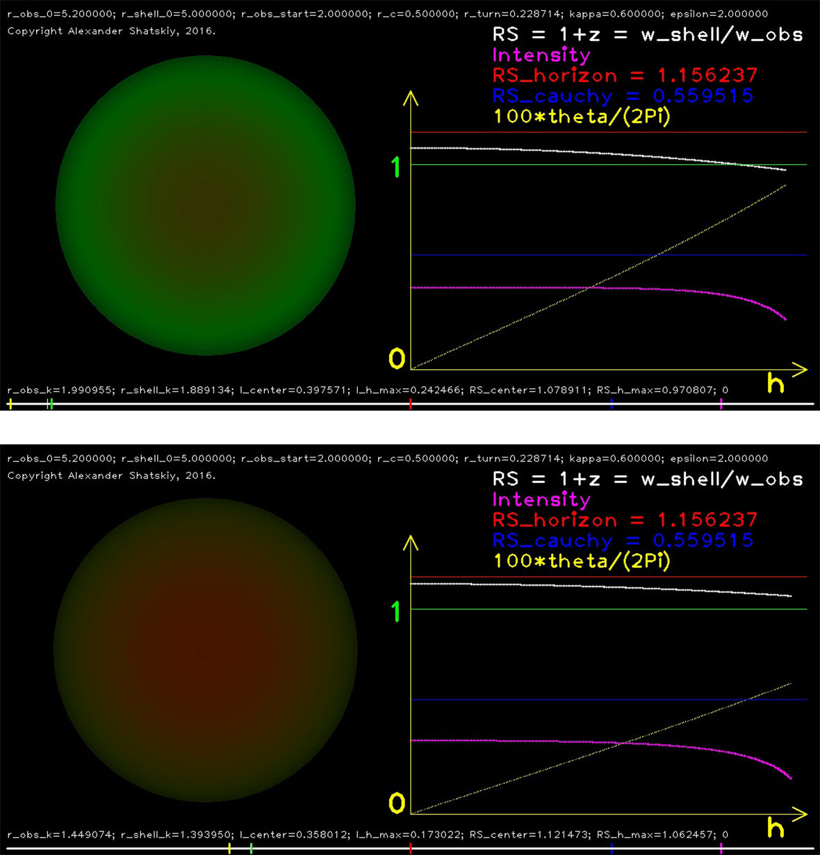 Figure 1
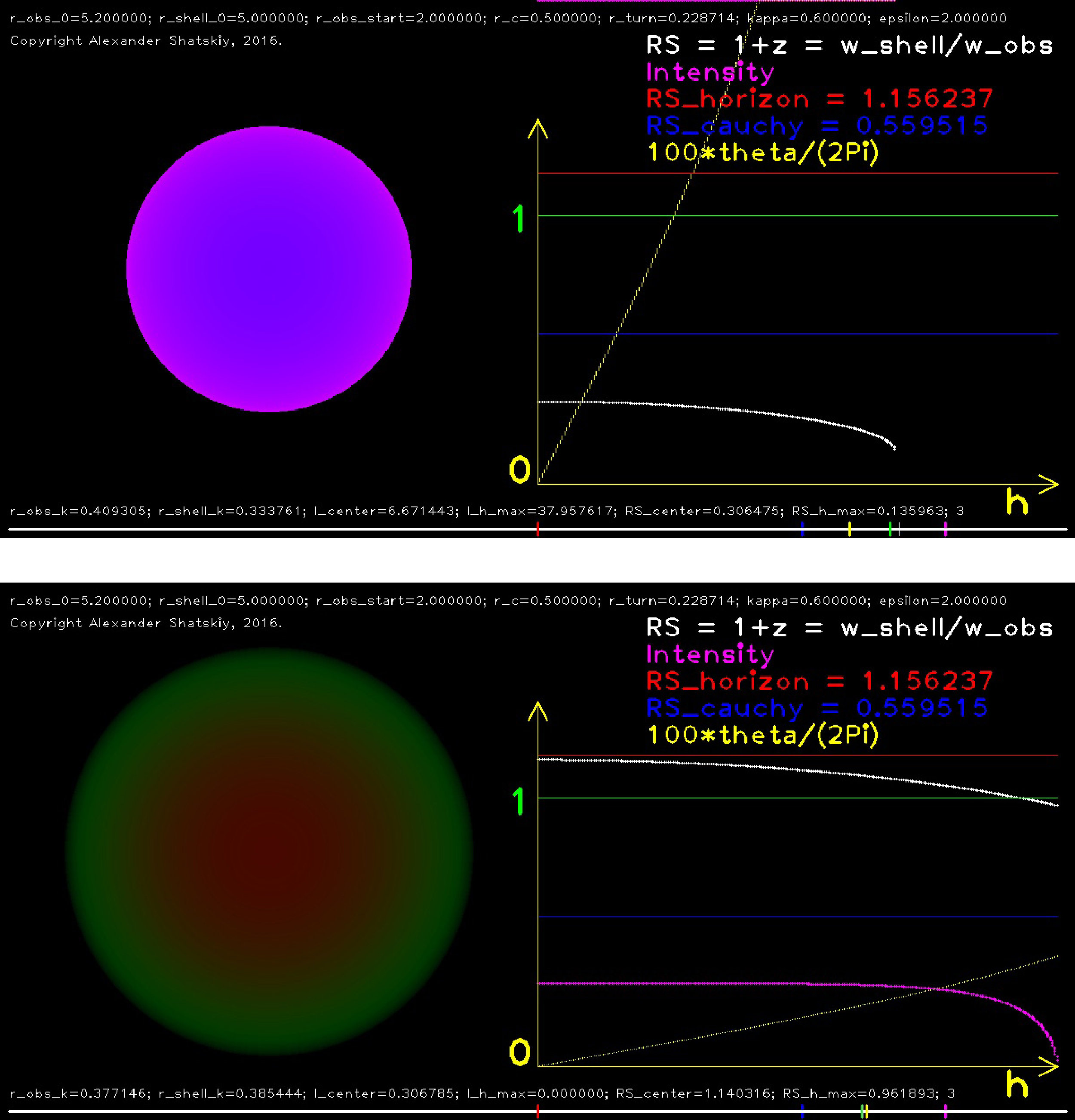 Figure 2
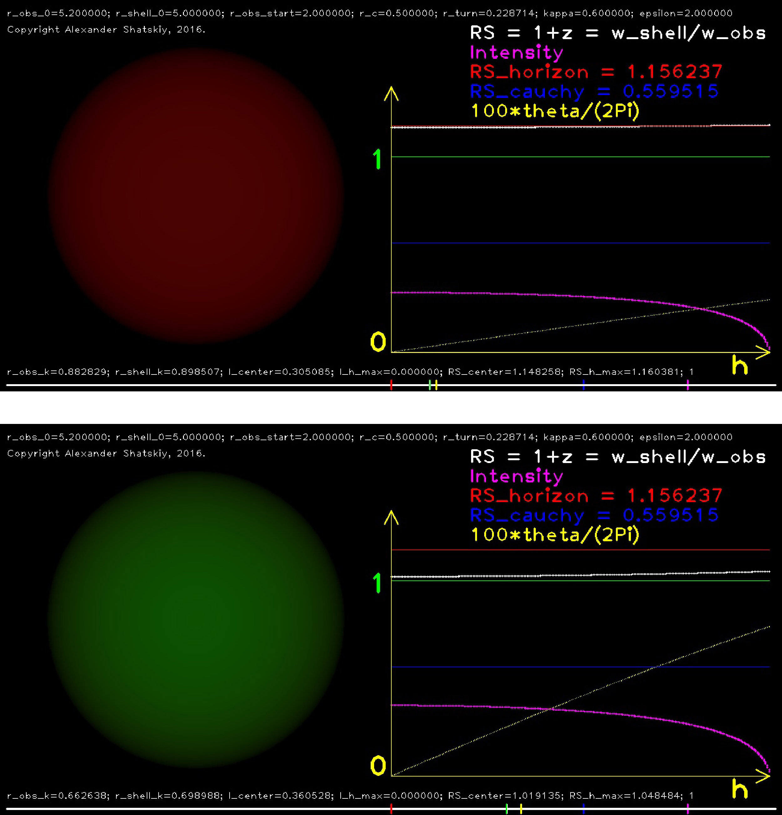 Figure 3
Peer Reviews
No public reviews on file for this paper yet. If you reviewed it on a platform where reviews are public (OpenReview, ICLR, NeurIPS, ICML), you can paste yours below so the community can read it here.
Videos
No videos yet. Explain this paper in a talk, walkthrough, or lecture? Add one.
\begin{picture}(178.0,10.0)\end{picture}
**A thin dust shell falling to a Reissner-Nordström black hole
as seen by a freely falling observer
**
**Alexander Shatskiy11footnotemark: 1
We study the observation of a thin dust shell, radially freely falling to a Reissner-Nordström black hole, by an observer who is also freely and radially falling into this black hole. Considered and resolved are several common paradoxes and fallacies peculiar for such problems. The results of this analytical study are written as a numerical code that allows for calculating all related effects of this model. The numerical result have been presented in a few synthesized videos, making a colorful, quantitative and detailed description of the occurring astrophysical phenomena, both above and below the horizon.
1 Introduction
Recently, my colleagues repeatedly encountered with misunderstanding and confusion in matters of hypothetically-possible observations of some effects from black holes. Moreover, this misunderstanding was sometimes originated by even professional astrophysicists. This concerns visual effects which accompany an observer freely falling into a black hole.
Of course, all these arguments are pure fantasy, in the sense of a possible technical implementation of such observations, but no doubt this subject is of methodological interest. This interest is related to understanding important effects of general relativity (GR) which accompany such hypothetic observations. This led to the idea to write an article in which these hypothetic observations would be described in detail and, most importantly, correctly.
In addition to the methodological study, description and calculation of this model, I have also made some virtual animations in which I tried to show exactly the real visual effects that must be seen by a freely falling observer (in theory). These videos are under open internet access. So, this work (with the videos) can be used for effective student learning as well as for all those interested in the subject.
Briefly about the model:
-
Let us imagine an observer freely falling into a black hole in vacuum, along the radius, and he is always in weightlessness.
-
In addition, a dust sphere fall into the black hole too, and the observer sees this sphere, which is closer to the black hole than the observer.
-
All dust particles of this sphere are at the same distance from the black hole at the same time. All dust particles also fall radially and freely.
-
The influence of the dust particles and the observer on the black hole is neglected.
A few words on the misconceptions. The main misconception, to be refuted in this paper, is that the observer should see an infinite red shift from the dust particles when the sphere reaches the black hole horizon.
The next misconception is that the observer will no longer see the radiation (the intensity tends to zero) when the sphere reaches the black hole horizon.
Let me briefly explain the cause of the above misconceptions. For photons near the horizon it is, in a sense, difficult to escape to infinity, it requires more time than far away from the horizon. Therefore an observer flying closer and closer to the horizon sees the photons that broke off the shell when it was only approaching the horizon, but the shell itself is at the same time already below the horizon. After crossing the black hole horizon, the observer falls to the center111Here and below, by the term “center” I mean a smaller radial coordinate than the location discussed. faster than for the photons from the dust, which are still “trying to get out,” but gravity “pulls” them to the center. And the observer, during the fall, still “comes across” these photons. For this reason the observer will not see any peculiarities when observing the photons from the shell, everything will look smooth and continuous!
Another common misconception is that under the horizon of a black hole we cannot use the Schwarzschild or Reissner-Nordström static coordinates – allegedly because below the horizon space and time interchange. The latter statement is fundamentally wrong: can only say that some properties are reversed in time and space, namely, the signs in the metric, but time still remains time and space remains space below the horizon.
Therefore, the static coordinates below the horizon can can be used, otherwise the conclusions on the existence of a singularity would be mistaken as well as the conclusions on the existence and location of the Cauchy horizon for real black holes. For a correct description of the observational effects below the horizon, it is necessary to write all formulas describing these effects in an invariant form, as is done in the following sections. As is known, the value of an invariant (or scalar) at a given point of space-time dos not depend on the choice of a coordinate system or reference frame.
In many other studies we have performed such calculations below the horizon in other frames, see [1–4]. Therefore, this choice of the coordinate system is not related to simplicity of calculations but is rather related to simplicity of interpretation and understanding. If we correctly repeat the further calculations, for example, in the comoving reference frame of freely falling matter, the results will be the same.
The Reissner-Nordström (electrically charged) black hole has been chosen as the original model. It is obvious that in space there cannot be objects with a large electric charge, so my choice of the Reissner-Nordström solution is associated with more fundamental reasons than simply a generalization of the Schwarzschild solution. It is associated with the fact that the Schwarzschild solution is unrealizable in nature: the real black holes always have some rotation, i.e., the real black holes are always Kerr black holes. At the same time, Kerr black holes have a nontrivial topology, fundamentally different from that of the Schwarzschild solution.
Due to the Cauchy horizon in the Kerr geometry, space-time splits into two internal areas, the T-region between the horizons and the R2-region under the inner horizon. The dynamics and observational manifestations of these interior regions are much more complex, interesting and multifaceted than for the single internal T-region in the Schwarzschild solution. However, the examination of the analytical and numerical models in the Kerr solution is much more difficult than in the Schwarzschild one. In the Kerr metric it is impossible to consider a spherical dust shell: it will be necessary bent and broken by gravimagnetic forces which are present in the Kerr solution. The maximum that could be considered in the Kerr solution analytically is the dynamics of a thin dust ring which falls and rotates in the equatorial plane of the Kerr coordinates. Therefore, the solution of this problem in the Reissner-Nordström metric is a compromise between reality and the complexity of the solution.
The consideration in the Reissner-Nordström metric has roughly the same complexity as in the Schwarzschild metric. It is the reason for choosing the Reissner-Nordström black hole, which, as well as the Kerr black hole, has a nontrivial topology and an inner Cauchy horizon, so that the Reissner-Nordström solution is closer to reality than the Schwarzschild simplest solution.
2 The laws of motion
The law of motion (the relation between time and the radius ) for a spherical thin dust shell, freely falls to a Reissner-Nordström black hole, in the Reissner-Nordström coordinates can be written in the general form
[TABLE]
where is some function to be determined further.
Similarly, for a photon in the same coordinates in the plane we can also write a law of motion:
[TABLE]
Here is the impact parameter of the photon which is directly related to the angle at which the photon was emitted from the shell; is some function for the photon, which will also be determined further.
Using Eq. (2), we obtain the time of radiation for a photon radially emitted from the shell with and :
[TABLE]
and the time for this photon to reach the observer:
[TABLE]
Since we consider only emitted photons (at different times) which reach the observer at the same time, we set this time equal to :
[TABLE]
The time of the radiation (to the observer) of a given photons corresponds to the radius of the shell, therefore, according to (1), we also have
[TABLE]
Here we have taken into account that earlier points in time correspond to larger radii and vice versa. Therefore, the integral in (6) should be negative because it must satisfy the condition that a photon with has time to reach the observer at the same time as a radial photon with . Since the nonradial photon needs more time it must be emitted before (at a larger radius).
The time of photon emission from the shell coincides (by definition) with the time , so from (2) and (6) we have
[TABLE]
Above, we assumed that the observer is located at radius at the moment of the arrival time of photons. But our observer is freely falling, so his coordinates (and the arrival time of photons) are also changing. To account for that, it is sufficient to replace all zero indices with the current index (such as the index : ). Then the zero index will be use as the initial conditions index of our model.
Let us choose the origin of time readout at . Then the integral (2) can be rewritten as
[TABLE]
Using this ratio, it is possible to calculate numerically the dependence for each index (i.e., for any time point for the observer).
At the same time, we believe that the time and the radius correspond to the radiation of the photon along the axis from the shell during its fall (and the arrival time of this photon to the observer at the moment ). By this time and by this radius , come all photons which have been nonradially emitted by the shell , they are radiated by the shell from radius , at the moments .
Differentiating both sides of Eq. (2) in the parameter , we get:
[TABLE]
Hence, we obtain the dependence .
3 Geodesic equations
We write the Reissner-Nordström metric:
[TABLE]
We use the geodesic equations for a particle moving in this gravitational field (see [5] or [6], § 87):
[TABLE]
Then for the metric (3) and for corresponding to the coordinate, we have the integral of motion: , and for corresponding to the coordinate, we have the integral of motion .
Given the identity , we have:
[TABLE]
Here, the minus sign before the root has been chosen according to the direction of motion, towards the center. Hence, for the radial fall of a massive particle we get the nonzero components :
[TABLE]
A transition to massless particles is accomplished by replacing in (3) and by the limiting transition :
[TABLE]
Here is the null 4-vector of the photon: ; the expression (3) is valid for a single photon, along its entire trajectory, and similarly to massive particles, and are integrals of motion for the photon. Similarly, the expression (3), plus sign in the expression (3) corresponds to the direction of photon emission from the center, and the minus sign to the center.
Knowing the 4-vectors, we obtain the function for massive particles and the function for photons:
[TABLE]
4 Redshift of a visible shell
In the reference frame comoving to a dust particle, the scalar product of the 4-vector for the photon and the velocity 4-vector of the observer is equal to the natural frequency of the photon: . Since the scalar product is an invariant, at the same point of the Reissner-Nordström system, we also have for the radiation frequency:
[TABLE]
In this case, the components of 4-velocity are the components of 4-velocity of dust particles in the Reissner-Nordström coordinates. Taking into account Eq. (3), the expression (16) on the dust shell can be rewritten as
[TABLE]
The plus sign in the expression (3) for has been chosen in accordance with the direction of photon emission from the center. Bear in mind that the denominator in the expression (17) vanishes on the horizon, and the expression becomes singular. This corresponds to the fact that the function for the emitted photon tends to zero (approach of the shell to the horizon). And for a photon directed towards the center (the minus sign in (3)), on the contrary, the singularity is subtracted, and the final frequency is everywhere finite (as well as the function ).
Similarly, from Eq. (17) at the observation point, the frequency measured by the observer is
[TABLE]
The Doppler shift is determined by the frequency ratio :
[TABLE]
It can be shown that the ratio is finite even near the horizon. To do that, we note that at approach to the horizon the function becomes small. The photon emitted by the shell at a radius is absorbed by the observer at the moment corresponding to the radius of the observer . And the function has the same order of smallness as the function for the same photon.
Let us assume (to simplify the calculations) that the value of for the observer is the same as for the dust shell, i.e., . Let us write the following equation:
[TABLE]
[TABLE]
Substituting the integrals (21)–(24) into Eq. (20) and reducing the intersecting areas of integration, we obtain:
[TABLE]
The value of determined from the initial conditions has the sense of time in the Reissner-Nordström system. During the time the photon emitted from the shell passes the distance to the observer’s position at the initial time and then, plus the time in which the observer flies the same distance (to the initial shell locations at ). However, this does not mean that we will have to start numerical integration of our model from the values of the radii and . We might as well begin numerical integration of our model at any values of the radii and which satisfy Eq. (4). Thus the initial assignment of values of the radii and determines the future relationship between the radii and from the integral in Eq. (4) for .
If, to both sides of Eq. (4), we add the following difference between the integrals:
[TABLE]
then Eq. (4) doesl not change, so the difference of the integrals in (26) should be zero.
To determine the redshift value, according to (4), it is sufficient to know two quantities: and . At the same time, the values of and are set by hand, and the values of and are calculated by the formula (26) — we integrate there to achieve its zero. The final point of integration in the second integral of (26) will be the required radius from which we find .
The value of the radius required for calculating and redshift of a photon with an arbitrary impact parameter , is calculated by Eq. (2), and the quantity necessary for that is also obtained from Eq. (23) by integration:
[TABLE]
In the limit , , , and , for the function we obtain the asymptotic behavior . Then the integral in (4) is also has the asymptotic behavior:
[TABLE]
Hence we have:
[TABLE]
Thus it is clear that the quantity
[TABLE]
is finite on the horizon,222Here we denote by the index the quantities at which we stop the numerical integration before the horizon . and therefore the redshift at the horizon is also finite:
[TABLE]
This shows that if or , then the frequency shift is red at the horizon.
Conclusion: Due to the choice of the static Reisner-Nordström coordinate system, we cannot pass continuously through the horizons points in our numerical integration. But the left and right limits of the expressions (4) are the same at the horizon, as well as the left and right limits of the ratio , therefore we can continue our integration after the horizon with the same limits as before the horizon.
These and further arguments are perfectly consistent with the membrane paradigm for black holes, see [7].
5 Discussion
Since all photons emitted upwards outside the horizon can be also observable only outside the horizons, and all photons emitted upwards between the horizons can be also observable only between horizons, these two regions are unconnected to each other (in the above sense).
In the external R1-region (up to falling into the black hole), as shown in (4), the redshift is determined only by the values of the radii and , the point of photon radiation and the point of its absorption. You could say that the redshift value is determined by the ratio of absolute values of , i.e., on the radii of photon radiation and absorption. Therefore, in the external R1-region the radial photon frequency will always decrease (redness). As for the nonradial photons (emitted with ), it needs more time (than for the radial photon) to reach the observer at the same time at which he/she receives the radial photon. Therefore, a nonradial photon must be emitted by the shell earlier, i.e., at a larger radius. This can lead to the fact that nonradial photons will experience blue (or violet) frequency shift when absorbed by the observer (for sufficiently large values of ). But in reality, these “blue” photons correspond to radiation inside by the shell (photons coming down).
In the T-region (between the horizons), amazing things begin to happen to our model! The outward emitted radial photon from the shell is trying to move upwards, but the gravity force is so great that it still moves down. After some time, the observer “catches” this photon… Thus it turns out that in the T-region the observation point has always has a smaller radius than that of the emission point (). Such “paradoxes” are only inherent to a T-region between the black hole horizons. Still the observer sees a redshift from the radial photons (in the early T-region).
Since the function is non-monotone in the T-region, the modulus reaches its maximum there and then decreases back to zero on the Cauchy horizon . Therefore, an instant will come when the functions will be the same for the emission point and the absorption. This will correspond to the absence of a frequency shift. After this instant, the situation will change — the observer will begin to see a blueshift of the frequency of radial photons. For nonradial photons the situation in this area is less predictable: everything depends on the radius (on the value of ) from which a nonradial photon comes to the observer.
For the same reasons as in the R1-region, nonradial photons need more time than the radial ones. Therefore they should be radiated by the shell at a larger radius (toward the outside horizon ). Therefore (due to a non-monotone function in the T-region) there can be variants with both redshifts and blueshifts of the frequency for nonradial photons.
However, there is one important remark: at once under the horizon , the observer cannot see a blueshift for any photons. This is due to the fact that all radiating shells (both for radial and nonradial photons) are at large radii (but under ), therefore the frequency shift will be only red. In this regard, immediately above the horizon (in the external R1-region) the frequency shift for the observer can only be red too because the observer can see only a continuous change in the frequency shift. It is possible that the observer before arriving at the horizon no longer sees such “blue” photons coming to him from inside the shell with sufficiently large values of .
In the interior R2-region (under the Cauchy horizon ), the situation once again radically changes. Now radial photons radiated up by shell can “overcome” the gravity force and move up to the incident observer. The observer will see these radial photons at a larger radius than at the radiation instant, but at lower values of the function . It will still conform to the blueshift for the radial photons. Now the observer in the R2-region can no longer see the photons emitted upward in the T-region because they “drift” down only to the Cauchy horizon and then remain on this horizon. Therefore, the observer sees only photons from the R2-region,333As was said above, the observer can see the photons (emitted upwards) only from the same region in which he is at the moment. and these are photons coming to him from large radii, closer to the Cauchy horizon . Thus, again, it can happen that a nonradial photon from the R2-region comes to the observer from a larger radius than the observer’s when watching it. In this case, the observer will see this nonradial photon as being red. Thus in the interior R2-region the observer will also be able to see both blue- and redshifted photon frequency (for sufficiently large ).
6 Motion between the horizons
All previous arguments and formulas remain the same in the T-region (between the horizons). Therefore, in Eqs. (21)–(26) it makes sense to replace the indices “0” with “h”, related to the horizon (the minus index means “under the horizon”). In the T-region, the sign of the expressions , , and changes to the opposite, it provides the necessary direction for the photons since the photons radiated outwards in this area “fly” to the center.
It is obvious (and verifiable in the the comoving reference frame) that an observer flying across the horizon , would not notice any shocks or peculiarities in the redshift of photons coming to him from the shell. Therefore, for the asymptotic behavior (just under the horizon ) we have , , , and . On the other hand, according to (29) and (30), we have:
[TABLE]
whence
[TABLE]
Therefore, to continue the numerical integration under the horizon , it is sufficient to take a small value of (and the corresponding radius , where the numerical integration was stopped in front of the horizon ), from Eq. (32) we obtain the radius , and with these values, we continue the integration, according to its analog in (26):
[TABLE]
In addition, it is possible to write an analog of Eq. (4):
[TABLE]
Similarly to the expression (31), from Eq. (34) in the limits and one can also express the ratio of the radii and (near the Cauchy horizon ):
[TABLE]
This shows that the frequency shift near the Cauchy horizon for radial photons will is blue-violet, i.e., the same as was predicted in the previous section.
7 Motion under the Cauchy horizon
In the R2-region (under the Cauchy horizon ) everything is similar to the previous arguments:
[TABLE]
Similarly to (35), we obtain
[TABLE]
The further integration can be continued up to the “throat”, the point , corresponding to the equation , see (13):
[TABLE]
After the throat point (in the dynamic Reissner-Nordström wormhole), matter starts expanding in the direction to another universe (in the topology of the total Reissner-Nordström multiverse, similar to what should happen in the Kerr solution). But these effects are beyond thge scope of this paper.
8 Distribution of energy flux density from the shell
The intensity (or more correctly to call it the energy flux density) is determined by the ratio of the photon flux which arriving at the observer (we consider only such photons) to the element of solid angle from which these photons are coming per unit natural time of the observer.
Consider an element of our dust shell in the range of angles from to (a thin ring with the radius ). The photon flux from this element is proportional to . The solid angle element at the observation point also lies in the range of angles from to , wherein the angle corresponds to the angle between the axis and the direction from which the photon has arrived. Therefore, the solid angle element at the observation point is .
Thus we obtain for the distribution :
[TABLE]
Here is the ratio of the elements of natural time of the observer and the shell, which is equal to the ratio of natural frequencies, see RS in (4). Another RS factor appears in (39) due to changes in the photon energy while traveling to the observer — it must also be taken into account in the calculation of the energy flux density. Therefore, to solve the problem, we need to introduce an invariant definition for the angles between the photons’ geodesic lines at their points of emission and absorption (separately).
Since we are interested in the angle between a radial geodesic () and a geodetic which has the impact parameter (at one and the same point), we need the following 4-vector:444The expression for the 4-vector contains the unit antisymmetric (in all four indices) tensor. Therefore (strictly speaking), this antisymmetric tensor should also be contracted with the antisymmetric kernel tensor
. At the contraction, we should take only the antisymmetric part of since the symmetric part of this tensor gives zero.
[TABLE]
Her,: , and , a unit, completely antisymmetric tensor of rank 4, see [6], §83; is the determinant of our metric tensor; is the radial velocity 4-vector of the observer or a dust particle of the shell; is the light 4-vector for a radial photon with ; is a null 4-vector of a non-radial photon with .
It can be seen that in our model the 4-vector has only one nonzero (axial) component
[TABLE]
Similarly, for the contravariant components of the 4-vector we have
[TABLE]
Hence we obtain the scalar :
[TABLE]
This shows that it makes sense to introduce one more 4-vector
[TABLE]
Then for the scalar we obtain the following invariant value:
[TABLE]
The value of by its physical meaning coincides with the square of the sine of the angle between the radial and non-radial null geodesics at radius . And the integral of motion does not change from the point of photon emission to the point of its absorption. The invariant expression (45) is just what we need since it is also true in the comoving, freely falling reference frame.
Then Eq. (39) can be rewritten in an invariant form:
[TABLE]
9 Boundary effects
If , the energy flux density (46) on the edges of the visible disk tends to infinity. It’s not an error! It is due to the fact that near the edge there are many dust rings of our shell which emit the photons to the observer. A similar effect can be seen, for example, while observing the Earth’s atmosphere from space: illuminated by the Sun, the atmosphere at the edge begins to shine brighter than at the center and becomes visible. However, if in our model we consider all dust rings to be completely opaque for light, then the expression (46) is multiplied by . But this is the other extreme. To take into account different options for the transparency of the dust rings, we introduce a coefficient in the expression for :
[TABLE]
Then corresponds to absolute opacity, and to absolute transparency of the dust rings.
The total angle of photon deflection while moving from the shell to the observer is determined by the expression (3):
[TABLE]
Thus the maximum possible impact parameter555This maximum possible impact parameter is not reached in our case, as can be seen from Eq. (47). for is determined by the relation , and in the T-region there can be any values of the impact parameters. For , the deflection angle of a photon will still be finite, despite the (weak) singularity in the denominator (48). This fact is fundamentally different from the observation of photons by an observer at rest in the Reissner-Nordström system. In this case, the photons’ deflection angles can reach infinity because for sufficiently large values of the photon makes an infinite number of turns around the black hole before it reaches the observer.
10 Visualization
As the main result of this work, I consider a program (code) due to which it is possible to synthesize videos illustrating how the dust shell will look like for a freely falling observer.
The videos of a Reissner-Nordström black hole with can be viewed at the addresses:
https://youtu.be/2PEJp8GOomY and
Videos for a Schwarzschild black hole can be viewed at the following addresses
https://youtu.be/0gfs-60mlQY and
The top and bottom of each video are presented with a string containing all current parameters of this video.
Visualization for the frequency shift RS on the video frames requires a detailed explanation.
The minimum light frequency perceived by human eye corresponds to the red color, and the maximum to violet. However, in technical devices (monitors and video projectors), all available colors are obtained by mixing the three color channels RGB (Red, Green and Blue), no violet color among them. Meanwhile, the violet color has the highest frequency in this visible light range, to the right of blue, therefore, apparently, it cannot be obtained by mixing other colors from the visible range. Paradoxically the human eye perceives an artificially synthesized violet color as a mixture in equal of red (R) and blue (B) channels (or colors). This fact makes some complexity in video synthesis, because the R and B channels correspond to almost opposite ends of the natural color spectrum visible by the human eye.
To make the mapping of colors in the videos maximally relevant to reality, it is reasonable to introduce the following assumption in the model: the shell emits only a monochrome line at natural frequency. I chose for this monochrome line pure green color (technically, there appears only one green channel, G).
With regard to the frequency shift to the red region, everything is fairly clear: I assigned the redshift on the black hole horizon to corresponds to the red channel R only. Between these two separate channels (G and R), there is a smooth frequency change, i.e., the R and G channels provide a smoothly varying contribution to the overall color picture.
For a further frequency shift to the violet region, I have assigned the color on the Cauchy horizon as a contribution from the blue channel B only. Between the horizons, the color gradually changes from pure red (only the R channel) to pure blue (only B) with a smooth passage through pure green (only the G channel, the natural frequency of the shell). Of course, at each point of the dust shell, this smooth color change will be of their own, smoothly and continuously connected with adjacent points. A further frequency increase occurs beyond the Cauchy horizon (i.e., reduction of the wavelength of light), therefore for zero wavelength I assigned an equal contribution from the red (R) and blue (B) channels, making the artificially synthesized violet color.
Of course, this synthetic color scheme is not fully consistent with what the human eye sees in reality, but this model maximally transfers all changes in the frequency shift from the monochrome green line emitted by dust particles. Moreover, one can observe not only by human eyes but (mostly) by technical means (cameras) which are known to work in different frequency bands.
Regarding visualization of radiation intensity, it is clear that for changing the intensity it is sufficient to synchronously change the contributions to the share in all channels (RGB), ranging from zero to 255 (maximally technically possible value).
On the right-hand side of the frame of all videos there are plots which synchronously change in time with the main picture: for the redshift values (the white curve), intensity (the violet curve) and the total deflection angle of photons (yellow curve), depending on the impact parameter of the photons.
In addition, the three horizontal solid lines are shown on the frames: the red one for the RS value on the event horizon , the green one indicating the unit, and the blue one for the RS value on the Cauchy horizon.
At the bottom, the scale of the observer radius is displayed (marked with a yellow label), that for the point of the dust shell nearest to the observer (a green label) and its maximally remote from the observer from which photons are coming to the observer (a white label), as well as the location of the event horizon (red label), the Cauchy horizon (blue label) and the throat (violet label).
11 Conclusion
All previous analytical arguments are confirmed by the numerical results displayed in the videos. These results show that the observer’s trip through both horizons and through the throat point proceeds smoothly and continuously, in particular, in the sense of observation of different elements of the dust shell.
Acknowledgments
I am sincerely grateful to Alexei Toporensky and Oleg Zaslavskii for all ideas, comments and discussions at the stage of preparation of this paper.
The reference list from the paper itself. Each links out to its DOI / PubMed record.
- 1[1] Alexander Shatskiy, JETP 104 (5), 743 (2007).
- 2[2] A. A. Shatskiy, A. G. Doroshkevich, D. I. Novikov, and I. D. Novikov, JETP 110 (2), 235 (2010).
- 3[3] A. Doroshkevich, J. Hansen, I. Novikov, Dong-Ho Park, and A. Shatskiy, Phys. Rev. D 81 , 129902 (2010).
- 4[4] N. S. Kardashev, L. N. Lipatova, I. D. Novikov, and A. A. Shatskiy, JETP 119 (1), 63 (2014).
- 5[5] G. C. Graves and D. R. Brill, Phys. Rev. 120 , 1507 (1960).
- 6[6] L. D. Landau and E. M. Lifshitz, The Classical Theory of Fields (Nauka, Moscow, 1988; Butterworth Heinemann, Oxford, 1990).
- 7[7] Kip S. Thorne, R. H. Price, and D. A. Macdonald (Eds.), Black Holes: The Membrane Paradigm (Yale University Press, New Heaven and London, 1986).