Interacting neutrinos in cosmology: exact description and constraints
Isabel M. Oldengott, Thomas Tram, Cornelius Rampf, Yvonne Y. Y., Wong

TL;DR
This paper provides an exact numerical analysis of neutrino self-interactions in cosmology, compares it with common approximations, and derives constraints on the interaction strength from current data, revealing a bimodal posterior distribution.
Contribution
It implements the exact Boltzmann hierarchy for interacting neutrinos into CLASS and compares results with existing approximations, providing new constraints on neutrino self-interaction strength.
Findings
Good agreement between exact approach and relaxation time approximation.
The popular $(c_{eff}^2,c_{vis}^2)$ parameterisation fails to capture scale dependence.
Cosmological data allow for two distinct neutrino interaction scenarios.
Abstract
We consider the impact of neutrino self-interactions described by an effective four-fermion coupling on cosmological observations. Implementing the exact Boltzmann hierarchy for interacting neutrinos first derived in [arxiv:1409.1577] into the Boltzmann solver CLASS, we perform a detailed numerical analysis of the effects of the interaction on the cosmic microwave background (CMB) anisotropies, and compare our results with known approximations in the literature. While we find good agreement between our exact approach and the relaxation time approximation used in some recent studies, the popular -parameterisation fails to reproduce the correct scale dependence of the CMB temperature power spectrum. We then proceed to derive constraints on the effective coupling constant using currently available cosmological data via an…
Click any figure to enlarge with its caption.
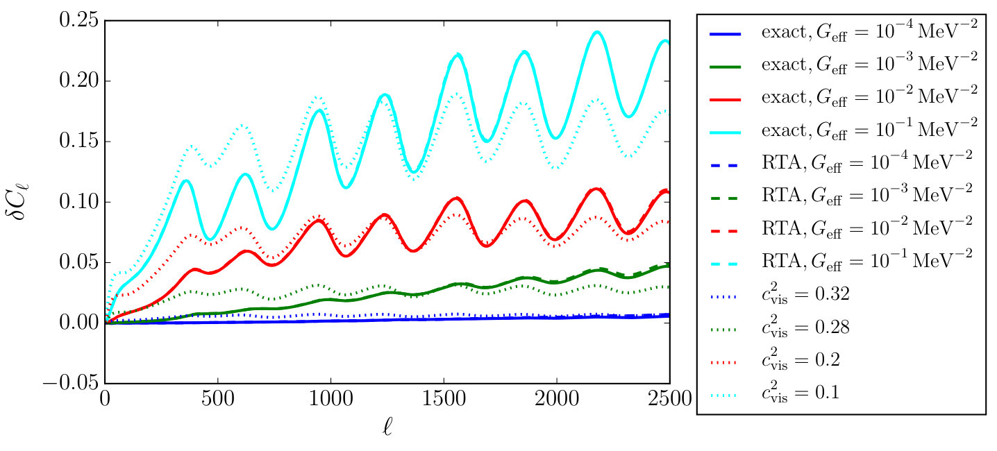 Figure 1
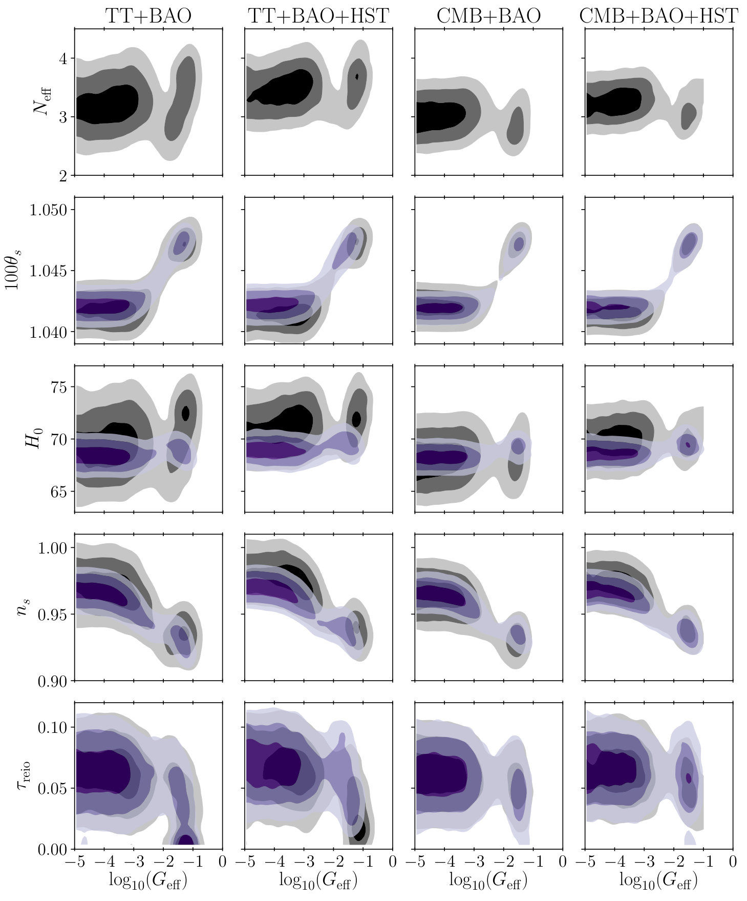 Figure 2
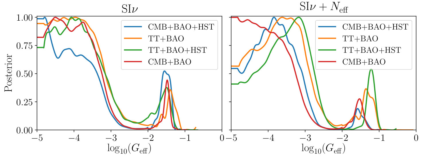 Figure 3
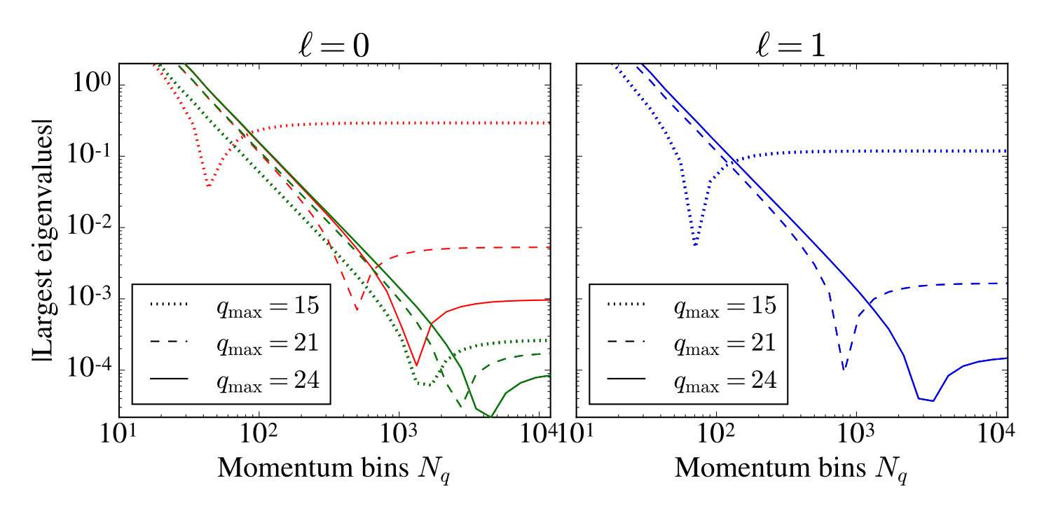 Figure 4
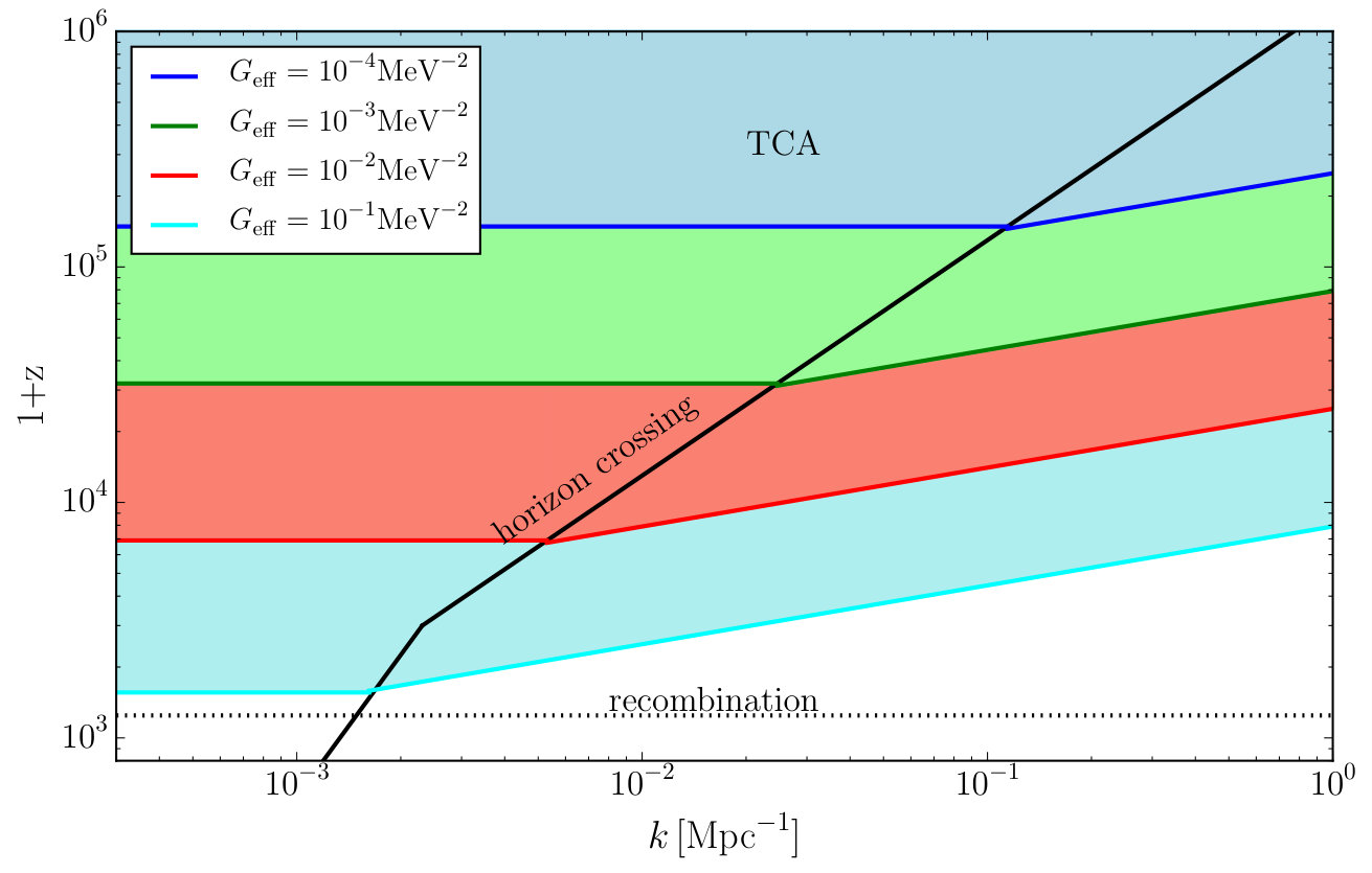 Figure 5
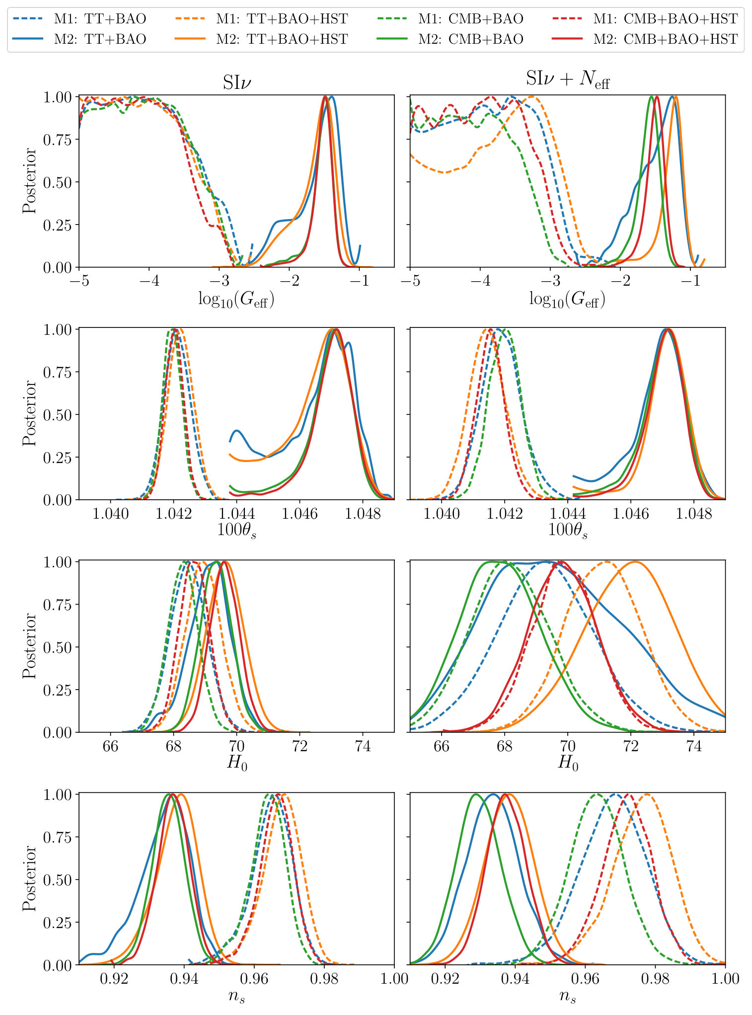 Figure 6
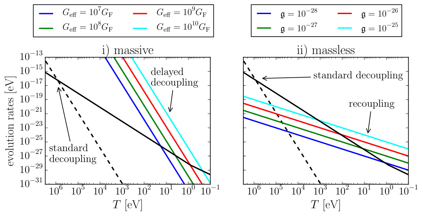 Figure 7
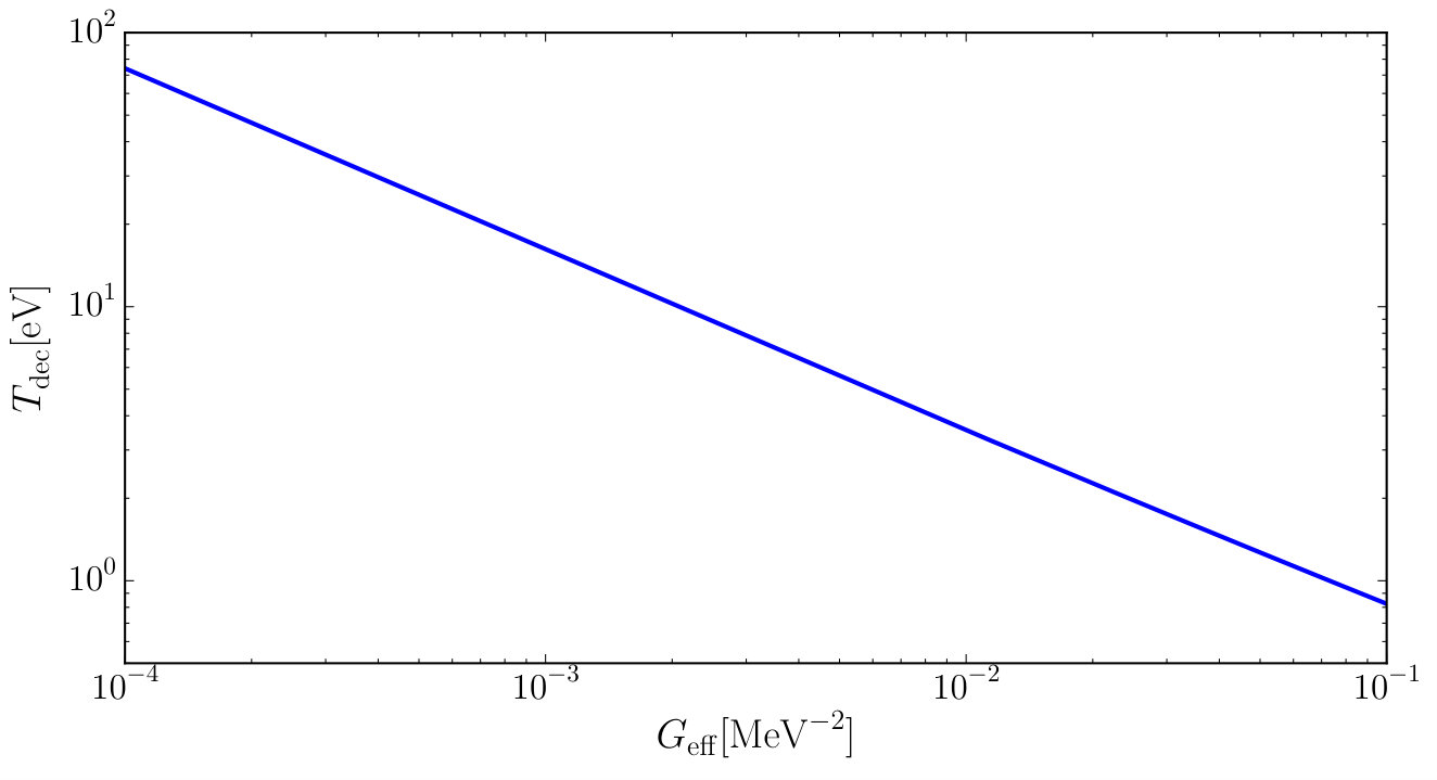 Figure 8
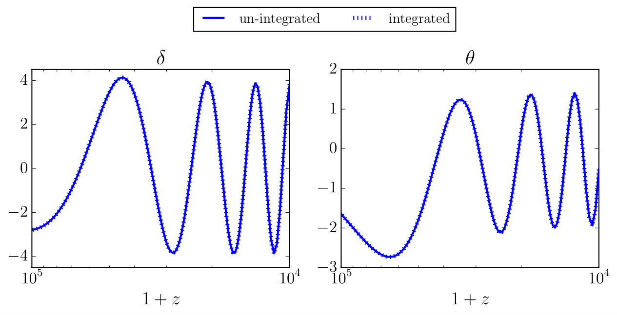 Figure 9
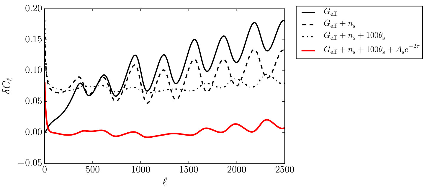 Figure 10
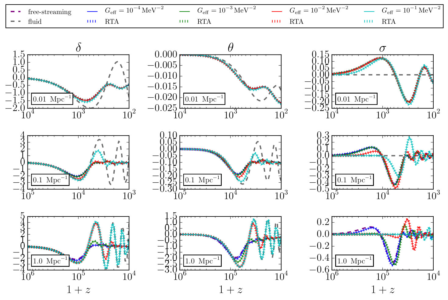 Figure 11
| M1 | M2 | |
|---|---|---|
| TT+BAO | TT+BAO+HST | CMB+BAO | CMB+BAO+HST | ||
|---|---|---|---|---|---|
| M1 | |||||
| M2 | |||||
| M1 | |||||
| M2 | |||||
| M1 | |||||
| M2 | |||||
| M1 | |||||
| M2 | |||||
| M1 | |||||
| M2 | |||||
| 4.5 | 2.9 | 3.4 | 0.9 | ||
| TT+BAO | TT+BAO+HST | CMB+BAO | CMB+BAO+HST | ||
|---|---|---|---|---|---|
| M1 | |||||
| M2 | |||||
| M1 | |||||
| M2 | |||||
| M1 | |||||
| M2 | |||||
| M1 | |||||
| M2 | |||||
| M1 | |||||
| M2 | |||||
| M1 | |||||
| M2 | |||||
| 4.9 | 3.5 | 2.6 | 1.8 | ||
Peer Reviews
No public reviews on file for this paper yet. If you reviewed it on a platform where reviews are public (OpenReview, ICLR, NeurIPS, ICML), you can paste yours below so the community can read it here.
Videos
No videos yet. Explain this paper in a talk, walkthrough, or lecture? Add one.
Interacting neutrinos in cosmology: exact description and constraints
Isabel M. Oldengott
Thomas Tram
Cornelius Rampf
and Yvonne Y. Y. Wong
Abstract
We consider the impact of neutrino self-interactions described by an effective four-fermion coupling on cosmological observations. Implementing the exact Boltzmann hierarchy for interacting neutrinos first derived in [1] into the Boltzmann solver class, we perform a detailed numerical analysis of the effects of the interaction on the cosmic microwave background (CMB) anisotropies, and compare our results with known approximations in the literature. While we find good agreement between our exact approach and the relaxation time approximation used in some recent studies, the popular -parameterisation fails to reproduce the correct scale dependence of the CMB temperature power spectrum. We then proceed to derive constraints on the effective coupling constant using currently available cosmological data via an MCMC analysis. Interestingly, our results reveal a bimodal posterior distribution, where one mode represents the standard CDM limit with , and the other a scenario in which neutrinos self-interact with an effective coupling constant .
1 Introduction
The nature of neutrinos and especially the mechanism by which they acquire masses constitute some of the most long-standing puzzles in particle physics. Because of the assumption that only left-handed neutrinos exist, neutrinos have been incorporated into the standard model (SM) of particle physics as exactly massless particles. However, the discovery of neutrino oscillations has long since refuted the assumption of exact masslessness. Besides providing a clear hint of physics beyond the SM, this also suggests that any extension to the SM to account for neutrino masses necessitates new coupling of the neutrino to particles as yet unobserved.
Numerous models of neutrino mass generation have been proposed in the literature. One interesting direction are majoron-like models in which a neutrino mass term is generated by the spontaneous breaking of a symmetry [2, 3, 4, 5, 6]. The symmetry breaking is accompanied by the appearance of a new Goldstone boson, called the majoron, that primarily couples to neutrinos via the Yukawa interaction,
[TABLE]
where and are, respectively, the scalar and pseudo-scalar couplings. Constraints on interactions of the type (1.1) have been derived from astrophysics (e.g., [7, 8]), big bang nucleosynthesis (e.g., [9]), neutrinoless double -decay (e.g., [10]), as well as the decay widths of the boson and certain mesons (e.g., [11, 12, 13]). Observations of the cosmic microwave background (CMB) temperature and polarisation anisotropies have so far provided useful insights into neutrino physics (e.g., limiting the sum of neutrino masses to eV [14]); it is therefore interesting to ponder if CMB measurements might also be sensitive to new neutrino interactions.
The generic signature of neutrino interactions during the time of CMB formation is an enhancement of its temperature power spectrum at multipoles following from a simple argument (see e.g. [15, 16, 17]). Non-interacting (and hence free-streaming) neutrinos in an inhomogeneous spacetime engender shear stress in the neutrino fluid, erasing fluctuations that might initially be present in the fluid and suppressing further growth. In contrast, neutrino interactions tend to isotropise the neutrino fluid locally, allowing its energy density contrast and velocity divergence to undergo acoustic oscillations in the sub-horizon limit. This in turn enhances the energy density and velocity contributions to the total gravitational source, and consequently the amplitude of the CMB temperature fluctuations on all scales that entered the horizon at times prior to photon decoupling.
While the limiting behaviours are well understood and their signatures easy to predict, the transition from fully interacting to non-interacting (or vice versa) is less clearcut. Several previous works have attempted to place CMB constraints on new neutrino interactions using a variety of heuristic arguments to model the equations of motion for the neutrino perturbations, the so-called “Boltzmann hierarchy”, in the transition region [15, 16, 18, 19, 20, 21, 22, 17]. Here, we take the view that once the interaction has been specified, the correct Boltzmann hierarchy should follow automatically from the collisional Boltzmann equation; the challenge lies in reducing the collisional integral to a numerically tractable form.
In a previous work [1], some of us determined the Boltzmann hierarchy in the presence of new neutrino interactions of the type (1.1) to first order in the perturbed quantities and in two limits of the scalar particle mass—extremely massive and effectively massless, relative to the typical energies of the neutrinos. In the present work we shall focus on the former, the “massive scalar” limit, wherein the interaction between two neutrinos becomes effectively a four-fermion interaction. We implement the corresponding neutrino Boltzmann hierarchy in the Boltzmann solver class [23], and present a detailed numerical analysis of the signatures of interacting neutrinos in the CMB anisotropies. We also take this opportunity to update the constraints on neutrino interactions using the 2015 data from the Planck CMB mission [14] and other recent cosmological observations.
The paper is organised as follows. We begin in section 2 with a review of the neutrino Boltzmann hierarchy first derived in [1], followed by a brief summary of other approaches in the literature. In section 3 we describe the implementation of the hierarchy in the Boltzmann solver class, and present for the first time numerical calculations of the CMB anisotropies in the presence of neutrino self-interactions using this approach. We derive constraints on the interaction strength from cosmological observations in section 4. Section 5 contains our conclusions.
2 Formalism
In a previous paper [1], some of us established the formal framework to study the impact of neutrino interactions on the CMB anisotropies in two limiting scenarios:
- (i)
The scalar mass far exceeds the typical energies of the neutrinos in the CMB epoch. In this limit the Lagrangian (1.1) becomes effectively a four-fermion interaction; any initial population of scalar particles will have decayed radiatively, and repopulation is kinematically suppressed. It therefore suffices to consider only the neutrino self-interaction , while treating the population as essentially non-existent. In this scenario, neutrinos decouple from the rest of the cosmic plasma at the weak decoupling temperature, but remain scattering with each other at an interaction rate per particle given by , assuming , where is the Fermi constant.
- (ii)
An effectively massless scalar relative to the typical energies of the neutrinos. With an interaction rate per particle of , the neutrinos in this scenario decouple at the weak decoupling temperature, free-stream for some time, and then recouple when overtakes the Hubble expansion rate , where is the Planck mass. Because the production of scalar particles is now kinematically possible, this scenario is a priori numerically far less tractable than the massive scalar case (i), and we shall not consider it in the present work.
The decoupling and, where applicable, recoupling behaviours of both limiting scenarios are illustrated in figure 1.
2.1 Neutrino Boltzmann hierarchy: Massive scalar limit
Following the notation of [24], and working in the synchronous gauge defined by the line element , the linear Boltzmann hierarchy for neutrinos interacting via the exchange of a very massive scalar particle is given by [1]
[TABLE]
Here, an overdot denotes a derivative with respect to the conformal time , and are, respectively, the trace and traceless perturbation of in Fourier space, and is the th Legendre moment, defined via
[TABLE]
of the phase space density , with and a Legendre polynomial of order .
In the collision terms, i.e., terms proportional to , note that for notational simplicity and in contrast to [1], we have absorbed the present-day neutrino temperature K into the definition of the comoving momentum variable . Accordingly, the integral kernels are now defined as
[TABLE]
where
[TABLE]
with the variables and . Furthermore, the normalisation factor , previously defined such that the background distribution matches the number density of a relativistic Fermi–Dirac distribution, is now defined to match the relativistic Fermi–Dirac energy density, i.e.,
[TABLE]
We also acknowledge here that, independently of these new definitions, a factor of had been omitted in front of the integral terms by oversight in [1].
Note that the equations of the Boltzmann hierarchy (2.1) must satisfy the conservation of number, energy, and momentum, which is reflected in the complete cancellation of their respective collision terms when integrated over momentum in the appropriate manner. These requirements can be used as a formal check of the correctness of the integral kernels (2.3). See appendix A for details.
Lastly, for completeness, we remind the reader that equation (2.1) has been derived under the assumption of (i) no Pauli blocking or Bose enhancement, (ii) Maxwell–Boltzmann distribution for non-degenerate background distribution functions, (iii) Majorana neutrinos that are ultra-relativistic in the timeframe of interest, and (iv) flavour-independent and diagonal scalar coupling, i.e., , and no pseudo-scalar coupling, i.e., . Modifying any one of these assumptions may substantially alter the form of the hierarchy.
2.2 Comparison to previous works
The salient feature of our “exact” Boltzmann hierarchy (2.1) is that it has a momentum dependence arising from the non-negligible energy transfer that accompanies a neutrino-neutrino scattering event. Such a momentum dependence does not appear in the Thomson scattering limit, and, to our knowledge, has been ignored in all earlier models of interacting neutrinos in cosmology. We briefly summarise these models below. A more detailed discussion can be found in [1].
-parameterisation
This most commonly-used model introduces two new parameters in the neutrino Boltzmann hierarchy, namely, an effective sound speed and a viscosity parameter . In the synchronous gauge, the modified hierarchy reads
[TABLE]
where we have used the notation of [24]. This parameterisation was first introduced in [25] to describe a generalised dark matter model, and reinterpreted in the context of neutrino interactions in, e.g., [20, 21, 22].
Setting in equation (2.6) reproduces the limit of free-streaming, non-interacting neutrinos, whereas the case of mimics the tightly-coupled limit—provided that the multipoles are initially unpopulated. This last condition on the multipoles should hold in the massive scalar scenario considered in this work, wherein neutrino decoupling is merely delayed by the new interaction. In the massless scalar scenario, however, the new interaction serves to recouple neutrinos that have already been free-streaming for some time, which clearly violates the condition on . Furthermore, in the context of an isolated ultra-relativistic system of particles, self-interacting or otherwise, any choice for other than would not comply with conservation of momentum, and is therefore not physically meaningful.
Doubts about the physical meaningfulness of the -model have been previously expressed in [1, 17, 26]. Indeed, we shall show in section 3.2 that not only does the parameterisation (2.6) have no formal interpretation in terms of particle scattering, it does not even reproduce the correct CMB phenomenology due to neutrino scattering.
Separable ansatz
In [17] a damping term proportional to the rate of change of the neutrino opacity, , is introduced in the neutrino Boltzmann hierarchy at orders , i.e.,
[TABLE]
where the s are model-dependent coefficients of order unity. The monopole and dipole equations remain unaltered on account of energy and momentum conservation. While equation (2.7) is clearly motivated by the first-order Boltzmann hierarchy for photons, we observe that it can be obtained from the exact Boltzmann hierarchy (2.1) by applying the ansatz that the phase space perturbation is independent of momentum, or, equivalently,
[TABLE]
Then, the two approaches are related simply by an integration in momentum. We call this the “separable ansatz”. See also [17].
The separable ansatz (2.8) also allows us to compare the exact Boltzmann hierarchy (2.1) with equation (2.7) in a meaningful way, as it enables us to compute explicitly the model-dependent coefficients . For a flavour-independent and diagonal interaction described by the scalar part of the Lagrangian (1.1), we find
[TABLE]
We shall use these coefficients when implementing equation (2.7) in class in section 3.
Note that equation (2.7) can also be motivated via the so-called relaxation time approximation (RTA, also sometimes referred to as the Bhatnagar–Gross–Krook approximation [27]), which assumes that the perturbed collision integral takes the form
[TABLE]
where is the time the system takes to relax to its equilibrium configuration. In fact, we note that the momentum-dependent version of equation (2.7), first presented in [28] in the context of self-interacting warm dark matter, used this approximation. Assuming a momentum-independent , it is easy to see that the RTA will lead to the Boltzmann hierarchy (2.7) upon integration in momentum. The RTA is often used in non-equilibrium physics to understand the basic features of thermalisation processes. It is, however, also known to be an incomplete description of the dissipative dynamics of generic systems of particles [29].
In the following we shall refer to the model (2.7) supplemented by the coefficients (2.9) as either the separable ansatz or the RTA.
3 Implementation
3.1 Boltzmann hierarchy on a momentum grid
We have implemented the exact Boltzmann hierarchy (2.1) in the Boltzmann solver class in order to study the impact of neutrino self-interactions on the CMB anisotropies. The implementation requires that we discretise the momentum variable , and numerically solve the Boltzmann hierarchy for each momentum bin . We describe in this section how this can be achieved in a numerically stable fashion.
The contribution to the perturbed energy-momentum tensor is obtained by summation over all momentum bins, e.g., the perturbed energy density of the neutrinos is given by
[TABLE]
where we have defined . The integral weights depend on the integration method used, and incorporate by definition the background distribution function of the neutrinos. For the present numerical implementation we have chosen a uniform momentum grid and a trapezoidal integration method. The discretised Boltzmann equation can then be written as
[TABLE]
where we have defined
[TABLE]
and
[TABLE]
is the scattering matrix encapsulating the collision kernels. At very early times, the -term is much smaller than the interaction term, and equation (3.2) becomes a homogeneous matrix equation with solution
[TABLE]
where we have expanded the integral around the initial time in the second line. The coefficients are fixed by the initial conditions, and and denote respectively the th eigenvalue and eigenvector of .
An intriguing feature of the scattering matrix in equation (3.4) is that, for small numbers of momentum bins , some eigenvalues at and can become positive—up to two at and one at . From equation (3.6) it is clear that any positive eigenvalue will cause to grow exponentially with conformal time for some time after the initial time, leading to a numerical instability for large values of . For smaller values, the system remains stable since the exact solution of equation (3.5) remains bounded. Such a behaviour is not physical, since the effect of the scattering should always be to damp the perturbation. Indeed, the positive eigenvalues at for small values are an artefact of a finite grid size. This is demonstrated in figure 2, where we show the absolute values of the largest eigenvalues of the matrices and as functions of . As we increase the eigenvalues decrease in magnitude, turn negative (the turnaround points correspond to the troughs in the curves), and finally reach their asymptotic values.
Clearly, to remove all positive eigenvalues from the equations would require several thousands of momentum bins. Needless to say, such a large number of momentum bins is not numerically feasible in a Boltzmann code. Furthermore, the values to which the eigenvalues asymptote depend on the chosen momentum cut-off scale in the discretisation, illustrated also in figure 2 by the sets of solid/dashed/dotted curves representing different values of . This, however, may be used to our advantage: since the magnitudes of the asymptotic eigenvalues appear to decrease with increasing , we may conclude that
[TABLE]
and on this basis implement the following routine:
We calculate the eigenvalues of the scattering matrix (3.4); 2. 2.
set the positive eigenvalues to their asymptotic () values, i.e., zero; and 3. 3.
derive a corrected scattering matrix, i.e., , where is the diagonal matrix with the corrected eigenvalues as diagonal entries, and is the matrix that diagonalises .
To make the system numerically stable it is furthermore very important to choose a sufficiently large value for , as too small a value of would cause the results to be dependent on . We have tested the above routine against different choices of and the cut-off momenta and , and found that choosing , , and suffices to obtain numerically stable solutions of the exact Boltzmann hierarchy (2.1).
3.2 Impact of interacting neutrinos on the CMB
Three phenomenological variables are relevant for the evolution of the neutrino perturbations, namely, the conformal Hubble rate , the comoving wavenumber , and the conformal interaction rate . The tightly-coupled approximation (TCA) holds whenever the interaction rate dominates over the other two, i.e., . In this case, multipole moments at in the neutrino Boltzmann hierarchy are strongly suppressed, so that only the equations in (2.1) or (2.7) need to be kept. Furthermore, as we show in appendix A, the collision terms of the exact Boltzmann hierarchy (2.1) vanish at and when integrated over momentum. This leaves
[TABLE]
as the only nontrivial equations of motion for the neutrino perturbations. In other words, interacting neutrinos can be described as a perfect fluid within the TCA. Figure 3 summarises the regions of validity of the TCA in the -plane for a range of values.
Holding fixed, we see in figure 3 that the TCA always fails first at large wavenumbers, followed by progressively smaller values until . Beyond this point, on super-horizon scales, the TCA formally fails for all at the same time. It is therefore useful to define a neutrino decoupling temperature, , as the temperature of the photons at which
[TABLE]
Evaluated explicitly for the radiation-domination era, we find
[TABLE]
where the numerical prefactors have been obtained using , and . Of course, neutrinos with different momenta decouple at different times. However, the measure (3.9) is still indicative of the average behaviour of the thermal ensemble (or, equivalently, the behaviours of momentum modes around ). Figure 4 shows as a function of the effective coupling constant . Note that the transition from radiation to matter domination in principle produces a change in the slope around eV; the change is however nearly impossible to resolve in the plot.
Figure 5 shows, following the notation of [24], the neutrino energy density contrast , velocity divergence , and shear stress at various wavenumbers, computed using our implementation of the exact Boltzmann hierarchy (2.1) in class, for different values of the effective coupling constant . For ease of comparison, solutions in the standard free-streaming limit and the fluid limit represented by equation (3.8) also appear in the figure. In all cases, apart from the parameters that describe the neutrino interaction, all other cosmological model parameters have been set to their Planck CDM best-fit values.
As expected, for very large values of , the perturbed quantities essentially track the fluid solutions at early times. This fact is particularly well illustrated by the case, where it is also apparent that the larger the value of , the longer the tracking period. When the conditions for TCA can no longer be satisfied, tracking ceases, accompanied by the generation of shear stress while power is being transferred to the higher multipoles of the Boltzmann hierarchy; the perturbed quantities eventually evolve to the standard free-streaming solutions. Finally, we also test in figure 5 the separable ansatz/RTA (2.7) against the exact Boltzmann hierarchy (solid lines vs short dashes): the agreement between the two approaches is, for all tested values and redshifts, very good.
Turning now to the impact of interacting neutrinos on the CMB anisotropies, figure 6 shows the relative difference in the temperature power spectrum,
[TABLE]
between an interacting scenario (“int”) and the standard free-streaming case (“CDM”). As expected, the larger the value of , the greater the relative difference engendered by neutrino interactions. Modulo the oscillations, for a given the greatest enhancement occurs on small angular scales (or large values of ). For coupling constants as large as, e.g., , neutrino interactions increase the CMB temperature power by almost 25% at . Conversely, the case of barely registers a 1% difference at . This also sets the ballpark for the scale of that can be probed using CMB measurements.
Comparing the relative differences computed using (a) our exact Boltzmann hierarchy (2.1), (b) the separable ansatz/RTA (2.7), and (c) the -parameterisation (2.6), we see in figure 6 that our exact approach and the separable ansatz/RTA yield essentially the same result.111For internal consistency we have used the model-dependent coefficients of equation (2.9) together with the separable ansatz/RTA (2.7). These coefficients are -dependent, and range from 0.40 to 0.48. However, we could equally have set them all to 1.0: save for a % difference in the definition of , these two choices of s have an almost identical impact on the CMB anisotropies. This comes as no surprise given the remarkable agreement between our exact approach and the separable ansatz already demonstrated in figure 5. We conclude therefore that the separable ansatz/RTA suffices to model the CMB phenomenology of neutrinos interacting via an effectively four-fermion vertex.
In contrast, modulo the oscillations, the -parameterisation produces a fairly uniformly enhanced temperature power spectrum at ; no matter what value we take as an input, the model clearly does not reproduce the full scale dependence of the exact approach or of the separable ansatz/RTA. We therefore conclude that the -parameterisation has neither a formal nor a phenomenological interpretation in the context of particle scattering, and hence should be avoided.
4 Constraints on the effective coupling constant
Given the demonstrated accuracy of the RTA in the massive scalar limit, we shall be working within this approximation in the following when testing neutrino self-interactions against cosmological observations in a Markov Chain Monte Carlo (MCMC) analysis.
4.1 Data sets
We use the following data sets in our analysis:
TT
Temperature power spectrum and low- polarisation from the Planck 2015 data [14].
CMB
Same as TT, but including also the -polarisation power spectrum (EE) and -polarisation cross-power spectrum (TE) from Planck 2015 [14].
BAO
Baryon acoustic oscillation peak scale as measured by 6DF [30], BOSS LOWZ and CMASS [31, 32], and the SDSS Main Galaxy Sample [33].
HST
Measurements of the local Hubble expansion rate by [34].
From these data sets we construct four different data combinations, all containing the TT and the BAO measurements: TT+BAO, CMB+BAO, TT+BAO+HST, CMB+BAO+HST.
4.2 Method
Using the MCMC engine Monte Python [35], we perform an MCMC analysis of two cosmological models containing self-interacting neutrinos:
SI: Comprises three species of massless neutrinos all interacting with strength . The parameters of the model are
[TABLE]
where is the sound horizon at recombination, and the other symbols carry their usual meanings. 2. 2.
SI+: Same as SI, but the number of self-interacting neutrino species, , is allowed to vary, thereby expanding the model parameter list to
[TABLE]
We assume flat priors on all of these parameters, and restrict the coupling constant to the range . Convergence of the Markov Chains is determined by the Gelman–Rubin convergence criterion .
For large couplings the system of equations becomes so stiff that even the implicit ODE-solver in class fails to evolve the system. This happens at . But even at class already becomes prohibitively slow. Therefore, in order to generate MCMC samples in a finite amount of time, we restrict the maximum number of steps allowed in the ODE-solver to . This restriction does not appear to have affected the SI-chains significantly, but the chains have been cut off at large values and .
Looking at figures 7 and 8 , it is also clear that a small second peak exists, in addition to the main peak at . This second peak was first pointed out in [17] and tentatively in [36] in their analyses of the Planck temperature measurements; the statistical significance was however low. Adding polarisation data and measurements of the local Hubble expansion rate substantially drives up the statistical significance of the second peak.
In order to properly sample the second peak, we increase the temperature of the chains by a factor of three, i.e., we sample the rescaled distribution . A further complication arises from the narrowness of the peak, which necessitates a small bin width and forces us to turn off spline-smoothing of the posteriors. Instead, we use a simple moving average smoothing in the part of the posterior, effectively increasing the bin-size in this part of the distribution by a factor of . Similar problems arise in the construction of the 2D contours, since the two islands are connected by an isthmus: applying a Gaussian smoothing with too large a smoothing scale would change the plot qualitatively by disconnecting the islands, so we must use a small smoothing scale.
As is evident in figure 8, the two peaks are most well separated in the parameter. We therefore divide up the parameter space in two modes, M1 and M2, along a plane of constant defined in table 1, and consider the two modes independently.
4.3 Discussions
Figure 9 shows the 1d posteriors for selected parameters in each mode, for both the and the model, derived from four data combinations TT+BAO, TT+CMB+BAO, CMB+BAO, and CMB+BAO+HST. In both models, the posterior of clearly shows that M2 is associated with large values of the effective coupling constant , while M1 corresponds to the non-interacting, free-streaming limit. Specifically, we find the constraints (see also tables 2 and 3):
[TABLE]
to be representative of , while for the same data combination yields a very similar
[TABLE]
In terms of the neutrino decoupling temperature (which can be read off figure 4 given a value), the M1 bound on translates approximately to a lowest decoupling temperature of eV, while the M2 peak corresponds to decoupling at eV.
Furthermore, as is evident in figure 9, M2 is accompanied by a lower spectral index and a higher sound horizon compared with M1. This result can be understood from figure 10, where we show the difference induced in the temperature anisotropy spectrum from variations of , , , and relative to the M1 mode. Firstly, the preference for a lower comes about because interacting neutrinos add power on small scales in a gradual manner that can be partially compensated by a redder spectral index. Secondly, the shift in the acoustic peaks due to the absence of neutrino anisotropic stress caused by a large can be partially cancelled by increasing . The simultaneous variation of , , and therefore results in a temperature anisotropy spectrum that closely mimics the free-streaming M1 mode, where the remaining offset can be easily touched up by adjusting the primordial fluctuation amplitude and optical depth to reionisation . Note also that these parameter degeneracies are only approximate; this explains the bimodality of the posterior distribution, because some values of can be better compensated than others. See also the discussion in section 5.1 of [37].
Observe that, in both models and especially , the -posterior in M2 does not drop to zero at the separation boundary for the TT+BAO data combination, indicating that the significance of M2 for this data combination is quite weak. Adding polarisation and HST data drives the posterior to zero at the boundary, producing a much more distinct M2 peak. Formally, the significance of M2 relative to M1 may be quantified via the -values at their respective best-fit points. These are tabulated in the last rows of tables 2 and 3, for and respectively. In both models and for all data combinations, we find M2 to be a worse fit to the data than M1, albeit only by a marginal for CMB+BAO+HST in the case of .
It is interesting to note in table 2 that, before the addition of HST data, the inferred value of the Hubble parameter in M2 of is approximately larger than in M1 of the same model. On its own this result is not enough to resolve the tension in between CMB and local measurements; it does however invite one to speculate if allowing to vary at the same time would further increase to the HST value. However, as is evident in figure 9 (and also in table 3), allowing to vary as well merely serves to draw the -posteriors of M1 and M2 closer to one another; there is no accompanying increase in the inferred value of .
The implications of M2 for the scalar spectral index are more interesting. As shown in figure 9, peaks in the range in the M2-mode for all data combinations. Such a low spectral index is completely excluded in the standard CDM model and, indeed, in most other extensions of CDM we are aware of. From the perspective of inflationary model building, could be realised, for example, by the Natural Inflation model [38, 39], where such a low value of would allow the symmetry breaking scale to be sub-Planckian, thereby rendering radiative corrections to the potential subdominant (see, e.g., figure 88 of [40]).
5 Conclusions
In this work, we have implemented into the Boltzmann solver class the exact Boltzmann hierarchy that describes neutrino self-interaction via an effective four-fermion coupling first derived in [1], and used it to investigate the phenomenology of the CMB in the presence of interacting neutrinos. Along the way we have also compared our exact approach with two other models used in the literature: the “separable ansatz” or relaxation time approximation (RTA), first introduced in [17], and the popular -parameterisation.
While the agreement between our exact approach and the separable ansatz/RTA is remarkable for this particular type of coupling, both at the level of the neutrino fluid perturbations (i.e., density contrast, velocity divergence, etc.) and at the level of the CMB angular power spectrum, we caution that this is not a statement on the validity of the separable ansatz/RTA in general. A self-interaction mediated by a massless scalar, for example, will most likely not respect the approximation, because the recoupling of neutrinos and especially their annihilation into scalars are expected to proceed in an energy-dependent fashion, causing the neutrino distribution to depart from a thermal shape for a period of time until the recoupling is complete.
The -parameterisation, on the other hand, is a poor model of neutrino scattering. Previous works have already cast doubts on the physical meaningfulness of the model [1, 17, 26]. In this work, we have shown explicitly that even at the purely phenomenological level, the model fails to predict the correct scale dependence for the CMB temperature power spectrum. Consequently, there is no meaningful way to map its model parameters to physical quantities such as the interaction strength. We therefore strongly advocate against using this model as a phenomenological description of particle scattering for CMB anisotropy calculations.
Using the RTA we have furthermore derived constraints on the effective coupling constant from cosmological observations in an MCMC analysis. Interestingly, all data combinations used in the analysis yield a bimodal posterior distribution, wherein one mode represents the standard CDM limit, and the other a scenario in which neutrinos self-interact with an effective coupling constant . The latter, “interacting” mode is accompanied by an inferred scalar spectral index in the ballpark , which may have interesting implications for inflationary model building.
Note added:
While this work was in its final stages of completion, the preprint [37] appeared on arXiv, which likewise presented cosmological constraints on neutrino self-interactions described by a four-fermion coupling. Although different methodologies have been applied, the results of [37] and our MCMC analysis are largely in agreement.
Acknowledgements
We thank N. Borghini, D. Boriero, S. Feld, D. Grin, S. Hannestad, D. Schwarz, T. Smith, and V. Vennin for interesting discussions. IMO acknowledges the support by Studienstiftung des Deutschen Volkes and by RTG 1620 “Models of Gravity” funded by DFG. TT acknowledges support from the Villum Foundation and computing resources from the Danish Center for Scientific Computing (DCSC). The work of CR is supported by the DFG through the Transregional Research Center TRR33 “The Dark Universe”. The work of Y3W is partially supported by the Australian Government through the Australian Research Council’s Discovery Projects funding scheme (project DP170102382).
Appendix A Proof of number-, energy- and momentum conservation
We demonstrate analytically in this appendix that the Boltzmann hierarchy (2.1) satisfies number, energy, and momentum conservation. In the case of the latter two, we furthermore show that our numerical implementation of (2.1) respects these conservation laws.
We begin the analytical proof by first writing down the full expressions for the collision kernels and according to equation (2.3):
[TABLE]
Conservation of number and energy density requires that the equation of (2.1) vanishes under the appropriate momentum integration, while for momentum conservation the condition of a vanishing momentum integral applies to the equation.
Number conservation
Here we integrate the equation (2.1) by . This yields for the first collision term
[TABLE]
Using from equation (A.1), the same integration over momentum produces for the second collision term
[TABLE]
which exactly cancels the first term (A.3).
Energy conservation
Integrating the equation over gives for the first collision term
[TABLE]
which cancels out the second collision term,
[TABLE]
upon momentum-integration.
Momentum conservation
Integrating the equation over leads to
[TABLE]
which is exactly cancelled by the second collision term,
[TABLE]
integrated over momentum in the same manner.
To demonstrate numerically that our implementation of (2.1) in class respects the conservation laws, we note first of all that numerical cancellation of the collision terms is most challenging for large couplings and large wavenumbers . In the former case, a large coupling causes the neutrino perturbations to undergo large-amplitude acoustic oscillations on sub-horizon scales, preserving power in the monopole and dipole. In the latter case, the larger the wavenumber, the earlier it crosses the horizon and hence the longer time it spends in oscillations (and at a higher frequency). See figures 3 and 5. We therefore conclude that if numerical cancellation of the collision terms occurs for the largest relevant and values in the tightly-coupled limit, then our implementation is more than sufficiently accurate for all other situations.
In its unintegrated form, the tightly-coupled limit of the Boltzmann hierarchy reads
[TABLE]
where upon integration in momentum we should recover the fluid equations (3.8). Thus, the solutions to equations (A.9) and (3.8) must yield the same and if energy and momentum conservation are respected numerically by our implementation. As shown in figure 11, in which we plot the evolution of and computed from both equations (A.9) and (3.8) for Mpc*-1* and MeV*-2*, this is indeed the case.
The reference list from the paper itself. Each links out to its DOI / PubMed record.
- 1[1] I. M. Oldengott, C. Rampf, and Y. Y. Y. Wong, “Boltzmann hierarchy for interacting neutrinos I: formalism,” JCAP 1504 (2015) no. 04, 016 , ar Xiv:1409.1577 [astro-ph.CO] . · doi ↗
- 2[2] G. B. Gelmini and M. Roncadelli, “Left-Handed Neutrino Mass Scale and Spontaneously Broken Lepton Number,” Phys. Lett. B 99 (1981) 411–415 . · doi ↗
- 3[3] K. Choi and A. Santamaria, “17-Ke V neutrino in a singlet - triplet majoron model,” Phys. Lett. B 267 (1991) 504–508 . · doi ↗
- 4[4] A. Acker, A. Joshipura, and S. Pakvasa, “A Neutrino decay model, solar anti-neutrinos and atmospheric neutrinos,” Phys. Lett. B 285 (1992) 371–375 . · doi ↗
- 5[5] Y. Chikashige, R. N. Mohapatra, and R. D. Peccei, “Are There Real Goldstone Bosons Associated with Broken Lepton Number?,” Phys. Lett. B 98 (1981) 265–268 . · doi ↗
- 6[6] H. M. Georgi, S. L. Glashow, and S. Nussinov, “Unconventional Model of Neutrino Masses,” Nucl. Phys. B 193 (1981) 297–316 . · doi ↗
- 7[7] K. C. Y. Ng and J. F. Beacom, “Cosmic neutrino cascades from secret neutrino interactions,” Phys. Rev. D 90 (2014) no. 6, 065035 , ar Xiv:1404.2288 [astro-ph.HE] . [Erratum: Phys. Rev.D 90,no.8,089904(2014)]. · doi ↗
- 8[8] K. Ioka and K. Murase, “Ice Cube Pe V–Ee V neutrinos and secret interactions of neutrinos,” PTEP 2014 (2014) no. 6, 061E 01 , ar Xiv:1404.2279 [astro-ph.HE] . · doi ↗