UConnRCMPy: Python-based data analysis for rapid compression machines
Bryan W. Weber, Chih-Jen Sung

TL;DR
UConnRCMPy is an open-source Python toolkit that streamlines the processing of rapid compression machine data, enabling consistent analysis of ignition delay and thermodynamic conditions for combustion research.
Contribution
It introduces a flexible, extensible Python package that standardizes RCM data analysis and facilitates reproducibility in combustion experiments.
Findings
Improves consistency in RCM data processing
Enables reproducible analysis workflows
Supports multiple experimental data formats
Abstract
The ignition delay of a fuel/air mixture is an important quantity in designing combustion devices, and these data are also used to validate chemical kinetic models for combustion. One of the typical experimental devices used to measure the ignition delay is called a Rapid Compression Machine (RCM). This paper presents UConnRCMPy, an open-source Python package to process experimental data from the RCM at the University of Connecticut. Given an experimental measurement, UConnRCMPy computes the thermodynamic conditions in the reaction chamber of the RCM during an experiment along with the ignition delay. UConnRCMPy implements an extensible framework, so that alternative experimental data formats can be incorporated easily. In this way, UConnRCMPy improves the consistency of RCM data processing and enables the community to reproduce data analysis procedures.
Click any figure to enlarge with its caption.
 Figure 1
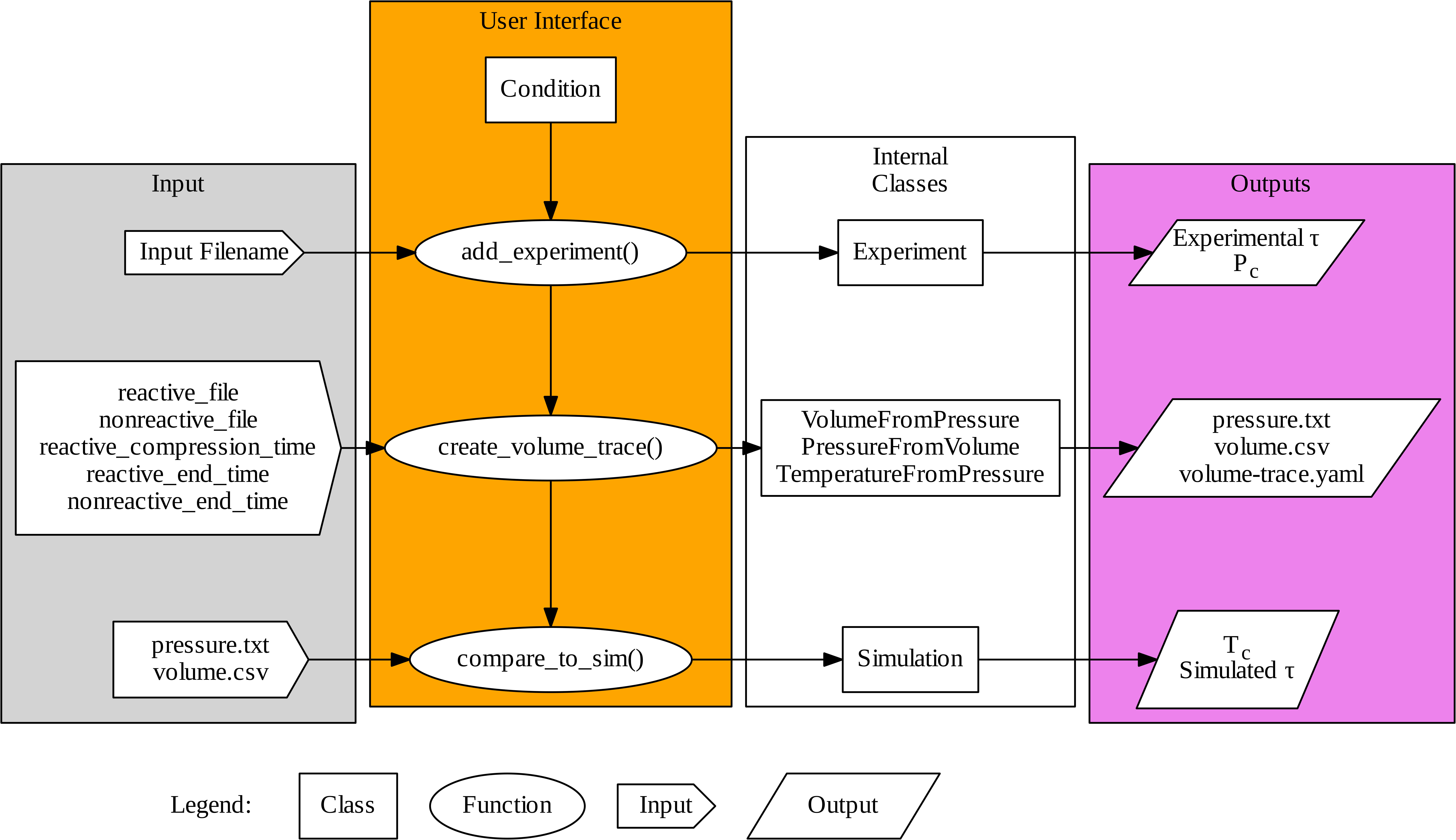 Figure 2
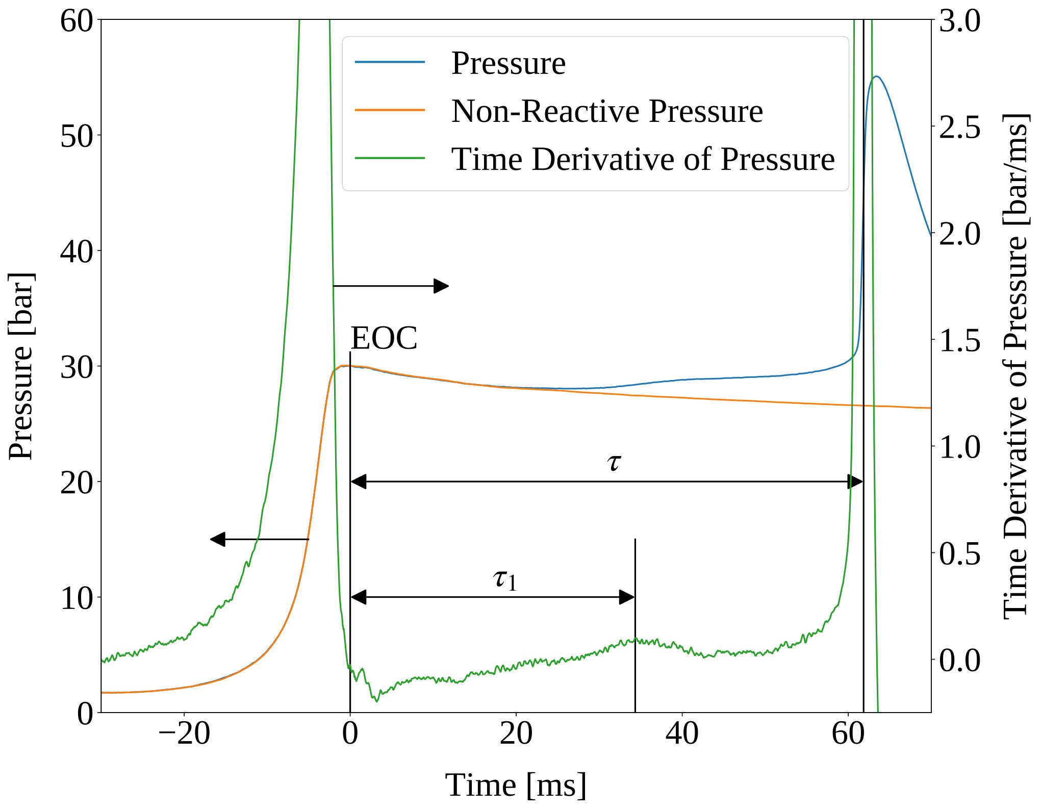 Figure 3
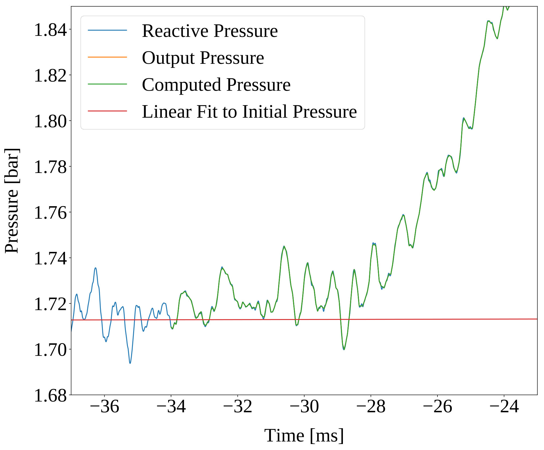 Figure 4
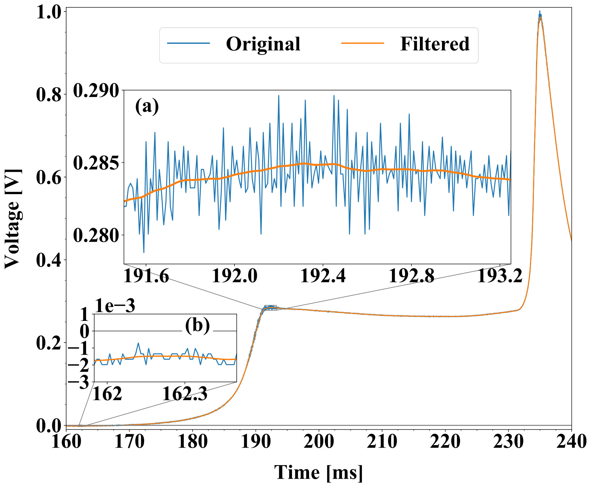 Figure 5
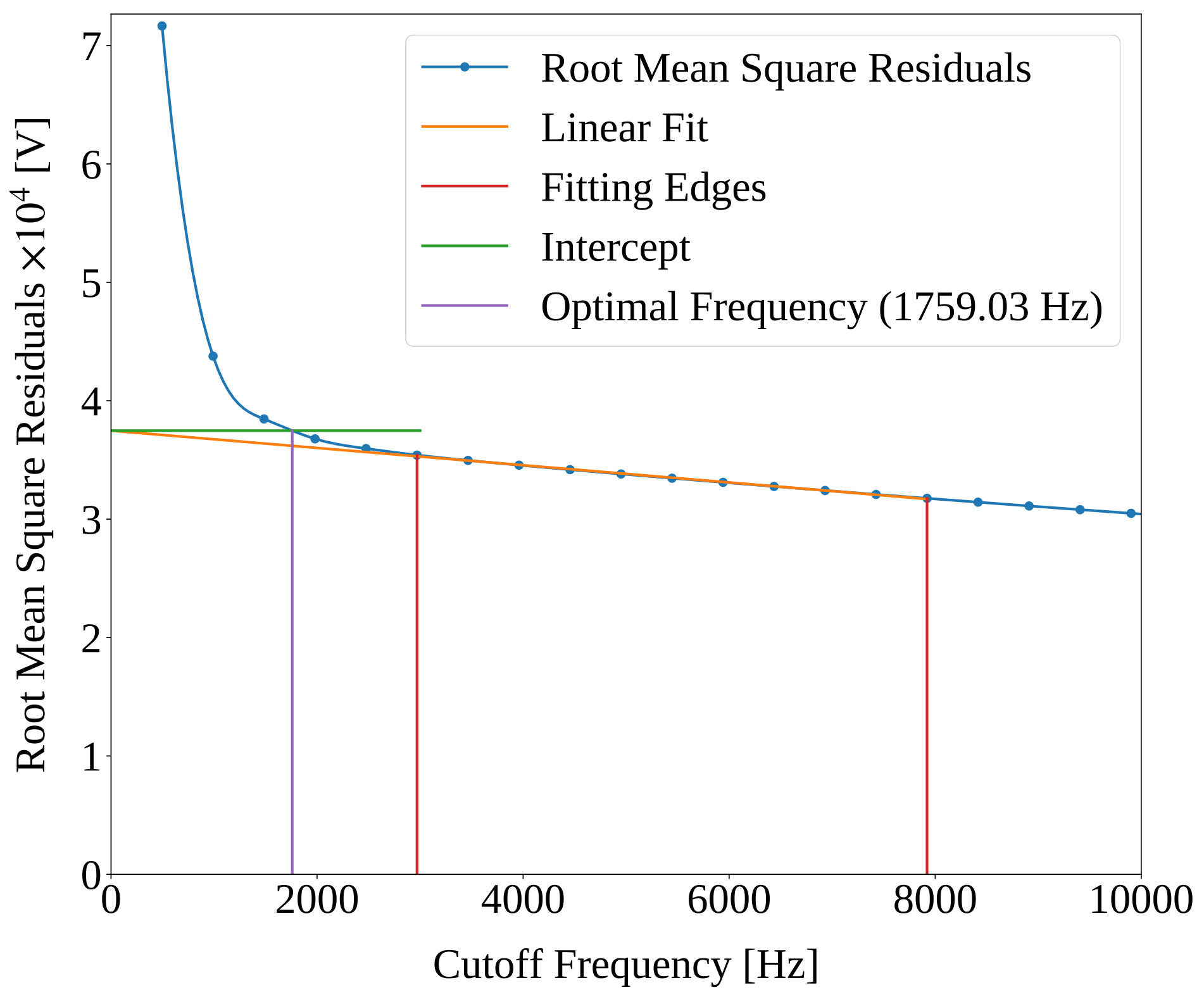 Figure 6
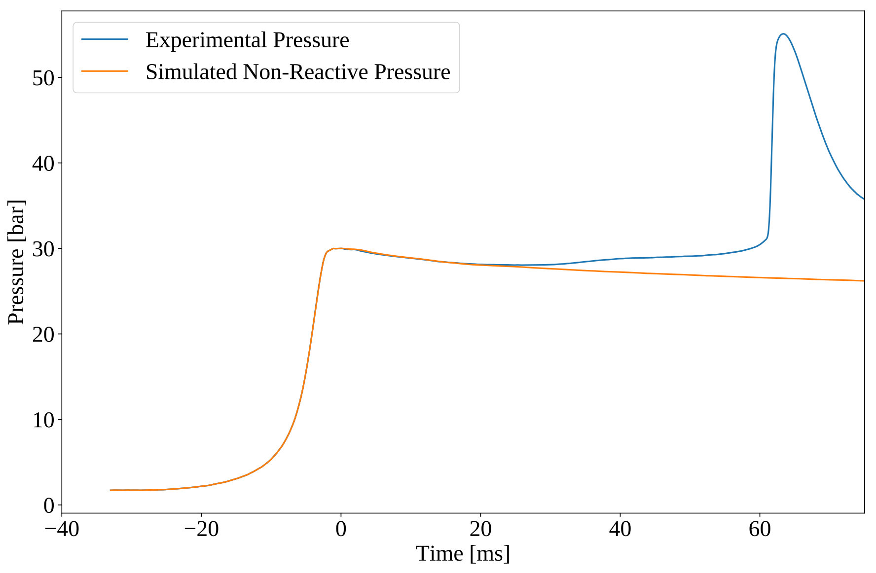 Figure 7
Peer Reviews
No public reviews on file for this paper yet. If you reviewed it on a platform where reviews are public (OpenReview, ICLR, NeurIPS, ICML), you can paste yours below so the community can read it here.
Videos
No videos yet. Explain this paper in a talk, walkthrough, or lecture? Add one.
\includexmp
CC_Attribution_4.0_International
UConnRCMPy: Python-based data analysis for rapid compression machines
Bryan W. Weber
Chih-Jen Sung
Department of Mechanical Engineering, University of Connecticut, Storrs, CT, USA
Abstract
The ignition delay of a fuel/air mixture is an important quantity in designing combustion devices, and these data are also used to validate chemical kinetic models for combustion. One of the typical experimental devices used to measure the ignition delay is called a Rapid Compression Machine (RCM). This paper presents UConnRCMPy, an open-source Python package to process experimental data from the RCM at the University of Connecticut. Given an experimental measurement, UConnRCMPy computes the thermodynamic conditions in the reaction chamber of the RCM during an experiment along with the ignition delay. UConnRCMPy implements an extensible framework, so that alternative experimental data formats can be incorporated easily. In this way, UConnRCMPy improves the consistency of RCM data processing and enables the community to reproduce data analysis procedures.
keywords:
chemical kinetics\seprapid compression machine\sepPython\sepdata analysis
1 Introduction
In recent years, there has been a surge in interest in ensuring that research outputs are reproducible across time and personnel [1]. Recognizing that the code used to process experimental data is an important part of the chain from observation to result and publication, this paper presents the design and operation of a software package to process the pressure data collected from Rapid Compression Machines (RCMs). Our package, called UConnRCMPy [2], is designed to analyze the data acquired from the RCM at the University of Connecticut (UConn). Despite the initial focus on data from the UConn RCM, the package is designed to be extensible so that it can be used for data in different formats while providing a consistent interface to the user. Thus, UConnRCMPy offers all of the features required to process standard RCM data including:
- •
Filtering and smoothing the raw voltage output generated by the pressure transducer
- •
Converting the voltage trace into a pressure trace using settings recorded from the RCM
- •
Processing the pressure trace to determine parameters of interest in reporting the experiments, including the ignition delay and machine-specific effects on the experiment
- •
Conducting simulations utilizing the experimental information to calculate the temperature at the end of compression (EOC)
Previous software used to analyze RCM data has generally been undocumented and untested code specific to the researcher conducting the experiments. Moreover, the software typically used to estimate the temperature in the experiments is difficult to integrate with the data processing code. To the best of the authors’ knowledge, UConnRCMPy is the first package for analysis of standard RCM data to be presented in detail in the literature, and it tightly integrates the temperature estimation routine into the workflow, reducing errors and inefficiencies.
2 RCM Signal Processing Procedure
The RCMs at the University of Connecticut have been described extensively elsewhere [3, 4], and interested readers are referred to those papers for further details. The primary diagnostic on the RCM is the reaction chamber pressure during and after the compression process, measured by a dynamic pressure transducer. The pressure trace is processed to determine the quantities of interest, including the pressure and temperature at the EOC, and respectively, and the ignition delay, . These values depend on the pressure and temperature prior to the start of compression ( and , respectively), in addition to the composition of the reactant mixture and the overall compression ratio of the RCM. A single compression-delay-ignition sequence is referred to as an experiment or a run and a set of experiments at a given and mixture composition is referred to as a condition.
The dynamic pressure transducer outputs a charge signal that is converted to a voltage signal by a charge amplifier with a nominal output of . In addition, the output range of is set by the operator to correspond to a particular pressure range by setting a “scale factor.” The voltage output from the charge amplifier is digitized by a hardware data acquisition system and recorded into a plain text file by a LabView Virtual Instrument. Figure 2 shows a typical voltage trace measured from the RCM at UConn and demonstrates the typical noise in the signal, which requires filtering and further processing to produce a useful pressure trace.
In the current version of UConnRCMPy [2], the voltage is filtered using a first-order Butterworth filter. The cutoff frequency of the filter is chosen automatically by a procedure described in the work of [5, 6]. Briefly, this procedure applies low-pass filters of varying cutoff frequencies to the signal and calculates the root mean square residual between the filtered signal and the original signal. Figure 2 shows a typical plot of the residuals versus the cutoff frequency and demonstrates that the residuals are nearly linear for a range of cutoff frequencies. This range tends to start near one-twentieth the Nyquist frequency, as demonstrated by the left-most line labeled “Fitting Edges” on Fig. 2. To determine the right edge of the linear region, a series of linear regressions of the residuals are performed. The -intercept of the regression with the highest coefficient of determination is used to choose the optimal cutoff frequency. The right-most line labeled “Fitting Edges” in Fig. 2 demonstrates a case where the end point set at times the Nyquist frequency produces the best fit. The optimal cutoff frequency is chosen as the frequency at the intersection of the -intercept and the residuals curve.
After filtering, the voltage trace is converted to a pressure trace by correcting for the offset from the nominal initial volage of apparent in Fig. 2b, multiplying the voltage by the scale factor from the charge amplifier, and adding the initial pressure . The result is a vector of time-varying pressure values that must be further processed to determine the time of the EOC and the ignition delay.
Once the pressure trace has been constructed, , , and can be calculated. In the current version of UConnRCMPy [2], the time of the EOC is determined by finding the local maximum of the pressure prior to ignition. Then, the ignition delay is determined as the time difference between the EOC and the point of ignition, where the point of ignition is defined as the inflection point in the pressure trace due to ignition. The inflection point is found by the maximum of the first derivative of the pressure with respect to time. In the current version of UConnRCMPy [2], the first derivative of the experimental pressure trace is computed by a second-order forward differencing method. The derivative is then smoothed by a moving average algorithm with a width of 151 points. This value for the moving average window was chosen empirically.
For some conditions, the reactants may undergo two distinct stages of ignition. These cases can be distinguished by a pair of peaks in the first time derivative of the pressure. For some two-stage ignition cases, the first-stage pressure rise, and consequently the peak in the derivative, are relatively weak, making it hard to distinguish the peak due to ignition from the background noise. This is currently the area requiring the most manual intervention, and one area where significant improvements can be made by refining the differentiation and filtering algorithms. An experiment that shows two clear peaks in the derivative is shown in Fig. 3 to demonstrate the definitions of the ignition delays.
The final parameter of interest presently is the EOC temperature, . This temperature is often used as the reference temperature when reporting ignition delays. In general, it is difficult to measure the temperature as a function of time in the reaction chamber of the RCM, so methods to estimate the temperature from the pressure trace are used. The detailed procedure used in UConnRCMPy is described in the work of [7], and an overview is given here.
In general, the temperature in the RCM reaction chamber as a function of time can be found by integrating the first law of thermodynamics for an ideal gas:
[TABLE]
where is the specific heat at constant volume of the mixture, is the specific volume, and are the specific internal energy and mass fraction of the species , and is time. In UConnRCMPy, Eq. 1 is integrated by Cantera [8].
Integrating Eq. 1 requires knowledge of the volume of the reaction chamber as a function of time. To calculate the volume as a function of time, it is assumed that there is a core of gas in the reaction chamber that undergoes an isentropic, constant composition compression [9]. The initial entropy of the gas mixture is calculated using Cantera [8]. Subsequently, the state of the mixture is fixed by using the entropy and measured pressure; from this information, the volume is calculated. The initial volume is arbitrarily taken to be 1.0\text{,}{\mathrm{m}}^{3}$$. The initial volume used in constructing the volume trace is arbitrary provided that the same value is used for the initial volume in the simulations described below. However, extensive quantities such as the total heat release during ignition cannot be compared to experimental values.
Two simulations can be triggered by the user that solve Eq. 1. In the first, the multiplier for all the reaction rates is set to zero, to simulate a constant composition (non-reactive) process. In the second, the reactions are allowed to proceed as normal. Only the non-reactive simulation is necessary to determine , which is defined as the simulated temperature at the EOC time.
When a reactive simulation is conducted, the user must compare the temperature traces from the two simulations to verify that the inclusion of the reactions does not change , validating the assumption of adiabatic, constant composition compression. Although including reactions during the compression stroke does not affect the value of , it does allow for the buildup of a small pool of radicals that can affect processes after the EOC [10]. Thus, it is critical to include reactions during the compression stroke when conducting simulations to compare a kinetic model to experimental results.
As can be seen in Fig. 3, the pressure decreases after the EOC due to heat transfer from the higher temperature reactants to the reaction chamber walls. This process is specific to the machine that carried out the experiments, and to the conditions under which the experiment was conducted. To include the effect of this heat transfer into simulations, a non-reactive experiment is conducted, where in the oxidizer is replaced with .
To apply the effect of the post-compression heat loss into the simulations, the reaction chamber is modeled as undergoing an isentropic volume expansion after EOC, and the same procedure is used as in the computation of to compute a volume trace for the post-EOC time. The only difference is that the non-reactive pressure trace is used after the EOC instead of the reactive pressure trace. This procedure has been validated experimentally by measuring the temperature in the reaction chamber during and after the compression stroke. The temperature of the reactants was found to be within \pm\sim$$5\text{\,}\mathrm{K} of the simulated temperature [11, 12].
3 Implementation and Usage of UConnRCMPy
UConnRCMPy is constructed in a hierarchical manner. The main user interface to UConnRCMPy is through the \pyboxCondition class, the highest level of data representation. The \pyboxCondition class contains all of the information pertaining to the experiments at a given condition. The intended use of this class is in an interactive Python interpreter (the authors prefer the Jupyter Notebook with an IPython kernel [13]). First, the user creates an instance of the \pyboxCondition class.
{pythonbox}
from uconnrcmpy import Condition
cond_00_02 = Condition(cti_file=’./species.cti’)
The \pyboxcti_file argument to \pyboxCondition must point to a file in the CTI format that contains the thermodynamic and reaction information for the species in the mixture. The experiments in the following example were conducted with mixtures of propane, oxygen, and nitrogen [7]. The CTI file necessary to run this example can be found in the Supplementary Material of the work by [7]. Then, the composition of the mixture under consideration must be added to the \pyboxinitial_state parameter of the \pyboxideal_gas() function in the CTI file:
{pythonbox}
ideal_gas( name=’gas’, elements=…, species=…, reactions=’all’, initial_state=state(mole_fractions=’C3H8:0.0403,O2:0.1008,N2:0.8589’))
Ellipses indicate input that was truncated to save space; the truncated input is present in the file available with the work of [7]. The \pyboxmole_fractions must be set to the appropriate values. The condition in this example is for a fuel rich mixture, with a target of .
After initializing the \pyboxCondition, the user conducts a reactive experiment with the RCM and adds the experiment to the \pyboxCondition using the \pyboxadd_experiment() method. As each experiment is processed by UConnRCMPy, the information from that run is added to the system clipboard for pasting into some spreadsheet software. In the current version, the information copied is the time of day of the experiment, the initial pressure, the initial temperature, the pressure at the EOC, the overall and first stage ignition delays, an estimate of the EOC temperature, some information about the compression ratio of the reactor, and the filter frequnecy used.
{pythonbox}
Conduct reactive experiment #1 on the RCM
cond_00_02.add_experiment(’00_in_02_mm_373K-1282t-100x-19-Jul-15-1633.txt’)
… conduct and add other reactive experiments
In general, for a given condition, the user will conduct and process all of the reactive experiments before conducting any non-reactive experiments. Then, the user chooses one of the reactive experiments as the reference experiment for the condition (i.e., the one whose ignition delay(s) and are reported) by inspection of the data in the spreadsheet. The reference experiment is defined as the experimental run whose overall ignition delay is closest to the mean overall ignition delay among the experiments at a given condition. To select the reference experiment, the user sets the \pyboxreactive_file attribute of the \pyboxCondition instance. For this case, the reference experiment is the run that took place at 16:33:
{pythonbox}
cond_00_02.reactive_file = ’00_in_02_mm_373K-1282t-100x-19-Jul-15-1633.txt’
Once the reference reactive experiment is selected, the user conducts experiments at the same initial pressure and temperature conditions, but with a non-reactive mixture. The user adds non-reactive experiments to the \pyboxCondition by the same \pyboxadd_experiment() method and UConnRCMPy automatically determines whether the experiment is reactive or non-reactive. If the user does not specify the \pyboxreactive_file attribute, they are prompted for the file name when the first non-reactive case is added.
{pythonbox}
Conduct non-reactive experiment #1 on the RCM
cond_00_02.add_experiment(’NR_00_in_02_mm_373K-1278t-100x-19-Jul-15-1652.txt’)
UConnRCMPy determines that this is a non-reactive experiment and generates a new figure that compares the current non-reactive case with the reference reactive case. For this particular example, the pressure traces are shown in Fig. 3. In this case, the non-reactive pressure agrees very well with the reactive pressure and no further experiments are necessary; in principle, any number of non-reactive experiments can be conducted and added to the figure for comparison. Since there is good agreement between the non-reactive and reactive pressure traces, the user sets the \pyboxnonreactive_file attribute of the \pyboxCondition instance.
{pythonbox}
cond_00_02.nonreactive_file=’NR_00_in_02_mm_373K-1278t-100x-19-Jul-15-1652.txt’
Once the non-reactive case is chosen, the \pyboxcreate_volume_trace() method can be run. This method requires three attributes to be set on the \pyboxCondition instance: \pyboxnonreactive_end_time which controls the end time for volume trace generation, \pyboxreactive_end_time which controls the length of the pressure trace stored in the output file, and \pyboxreactive_compression_time which is the length of the compression stroke. All of the values must be supplied in units of milliseconds.
{pythonbox}
cond_00_02.nonreactive_end_time = 400 cond_00_02.reactive_end_time = 80 cond_00_02.reactive_compression_time = 36
After generating the volume trace, \pyboxcreate_volume_trace() writes the \pyboxvolume.csv file, the pressure trace file, and a file called \pyboxvolume-trace.yaml, which contains the values that were set for each attribute. The final step to conduct the simulations to calculate and the simulated ignition delay. This is done by the user by running the \pyboxcompare_to_sim() function. This function takes two optional arguments, \pyboxrun_reactive and \pyboxrun_nonreactive. These determine which type(s) of simulation(s) should be conducted.
{pythonbox}
cond_00_02.create_volume_trace() cond_00_02.compare_to_sim(run_reactive=True, run_nonreactive=True)
UConnRCMPy is documented using standard Python docstrings for functions and classes. The documentation is converted to HTML files by the Sphinx documentation generator [14]. The format of the docstrings conforms to the NumPy docstring format so that the autodoc module of Sphinx can be used. The documentation is available on the web at https://bryanwweber.github.io/UConnRCMPy/. UConnRCMPy also relies heavily on functionality from the NumPy [15], SciPy [16], and Matplotlib [17] Python packages.
4 Conclusions and Future Work
UConnRCMPy provides a framework to enable consistent analysis of RCM data. Because it is open source and extensible, UConnRCMPy can help to ensure that RCM data in the community can be analyzed in a reproducible manner; in addition, it can be easily modified and used for data in any format. In this sense, UConnRCMPy can be used more generally to process any RCM experiments where the ignition delay is the primary output.
Future plans for UConnRCMPy include the development of a robust test suite to prevent regressions and document correct usage of the framework, as well as the development of a plugin architecture to allow easy implementation of user-defined analysis features. Other issues and directions are listed in the Issue page of the GitHub repository https://github.com/bryanwweber/uconnrcmpy/issues/.
5 Acknowledgements
This paper is based on material supported by the National Science Foundation under Grant No. CBET-1402231.
The reference list from the paper itself. Each links out to its DOI / PubMed record.
- 1[1] “Reality Check on Reproducibility” In Nature 533.7604 , 2016, pp. 437–437 DOI: 10.1038/533437 a · doi ↗
- 2[2] Bryan William Weber, Ruozhou Fang and Chih-Jen Sung “U Conn RCM Py”, 2017 DOI: 10.5281/zenodo.321427 · doi ↗
- 3[3] Apurba Kumar Das, Chih-Jen Sung, Yu Zhang and Gaurav Mittal “Ignition Delay Study of Moist Hydrogen/Oxidizer Mixtures Using a Rapid Compression Machine” In Int. J. Hydrog. Energy 37.8 , 2012, pp. 6901–6911 DOI: 10.1016/j.ijhydene.2012.01.111 · doi ↗
- 4[4] Gaurav Mittal and Chih-Jen Sung “A Rapid Compression Machine for Chemical Kinetics Studies at Elevated Pressures and Temperatures” In Combust. Sci. Technol. 179.3 , 2007, pp. 497–530 DOI: 10.1080/00102200600671898 · doi ↗
- 5[5] Bing Yu, David Gabriel, Larry Noble and Kai-Nan An “Estimate of the Optimum Cutoff Frequency for the Butterworth Low-Pass Digital Filter” In J. Appl. Biomech. 15.3 , 1999, pp. 318–329 DOI: 10.1123/jab.15.3.318 · doi ↗
- 6[6] Marcos Duarte “Residual Analysis to Determine the Optimal Cutoff Frequency” In Jupyter Notebook Viewier , 2014 URL: http://nbviewer.jupyter.org/github/demotu/BMC/blob/master/notebooks/Residual Analysis.ipynb
- 7[7] Enoch E. Dames, Andrew S. Rosen, Bryan W. Weber, Connie W. Gao, Chih-Jen Sung and William H. Green “A Detailed Combined Experimental and Theoretical Study on Dimethyl Ether/Propane Blended Oxidation” In Combust. Flame 168 , 2016, pp. 310–330 DOI: 10.1016/j.combustflame.2016.02.021 · doi ↗
- 8[8] David G. Goodwin, Harry K. Moffat and Raymond L. Speth “Cantera: An Object-Oriented Software Toolkit for Chemical Kinetics, Thermodynamics, and Transport Processes”, 2017 DOI: 10.5281/zenodo.170284 · doi ↗