Nature vs. Nurture in Discrete Spin Dynamics
D.L. Stein

TL;DR
This paper reviews the predictability of spin dynamics in Ising systems after a deep quench, focusing on the final state nature and the influence of initial conditions versus system history, through analytical and numerical studies.
Contribution
It synthesizes existing analytical and numerical results on spin flip behavior and information dependence in Ising models, highlighting open problems in the field.
Findings
Some spins flip infinitely often, others finitely often, depending on system conditions.
Final state information depends variably on initial states and system history.
Open problems remain in understanding the full predictability of spin dynamics.
Abstract
The problem of predictability, or "nature vs. nurture", in both ordered and disordered Ising systems following a deep quench from infinite to zero temperature is reviewed. Two questions are addressed. The first deals with the nature of the final state: for an infinite system, does every spin flip infinitely often, or does every spin flip only finitely many times, or do some spins flip infinitely often and others finitely often? Once this question is determined, the evolution of the system from its initial state can be studied with attention to the issue of how much information contained in the final state depends on that contained in the initial state, and how much depends on the detailed history of the system. This problem has been addressed both analytically and numerically in several papers, and their main methods, results, and conclusions will be reviewed. The discussion closes with…
Click any figure to enlarge with its caption.
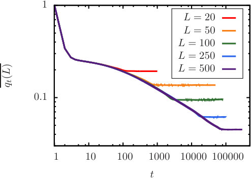 Figure 1
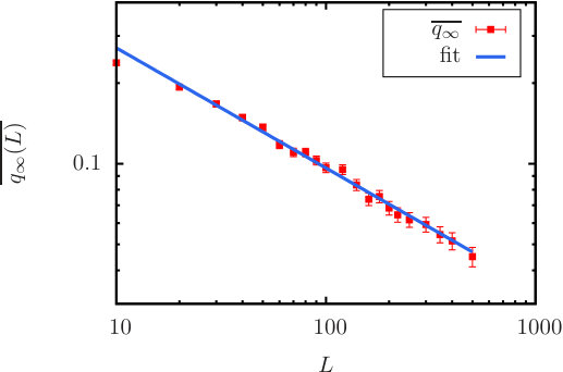 Figure 2
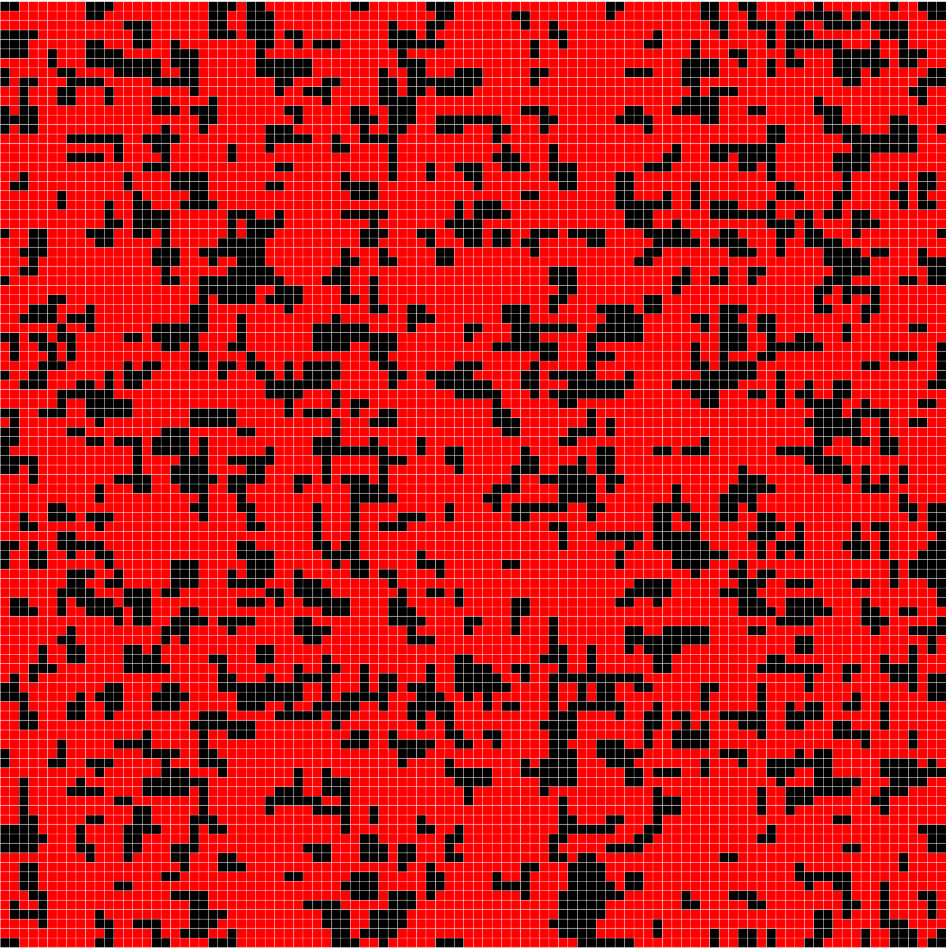 Figure 3
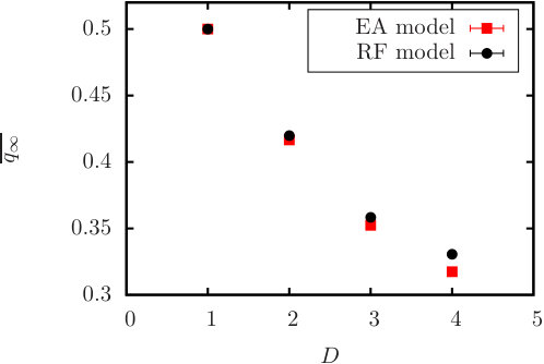 Figure 4
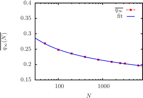 Figure 5
Peer Reviews
No public reviews on file for this paper yet. If you reviewed it on a platform where reviews are public (OpenReview, ICLR, NeurIPS, ICML), you can paste yours below so the community can read it here.
Videos
No videos yet. Explain this paper in a talk, walkthrough, or lecture? Add one.
Taxonomy
TopicsTheoretical and Computational Physics · Quantum many-body systems · Opinion Dynamics and Social Influence
Nature vs. Nurture in Discrete Spin Dynamics
D.L. Stein
Department of Physics and Courant Institute of Mathematical Sciences, New York University, New York, NY 10012 USA and NYU-ECNU Institutes of Physics and Mathematical Sciences at NYU Shanghai, 3663 Zhongshan Road North, Shanghai, 200062, China
Abstract
The problem of predictability, or “nature vs. nurture”, in both ordered and disordered Ising systems following a deep quench from infinite to zero temperature is reviewed. Two questions are addressed. The first deals with the nature of the final state: for an infinite system, does every spin flip infinitely often, or does every spin flip only finitely many times, or do some spins flip infinitely often and others finitely often? Once this question is determined, the evolution of the system from its initial state can be studied with attention to the issue of how much information contained in the final state depends on that contained in the initial state, and how much depends on the detailed history of the system. This problem has been addressed both analytically and numerically in several papers, and their main methods, results, and conclusions will be reviewed. The discussion closes with some open problems that remain to be addressed.
I Introduction
It is a great pleasure to contribute to this volume in honor of Chuck Newman’s birthday. Chuck has made so many fundamental contributions to probability theory, mathematical statistical mechanics, percolation theory, and many related fields that it was difficult to choose which topic to write about. The problem was resolved by settling on a problem of longstanding interest to Chuck, and one in which he remains heavily involved: the nonequilibrium dynamics of interacting spin systems, in particular following a deep quench, in which a system at high temperature is rapidly cooled to low temperature, after which it evolves according to equilibrium dynamics.
Our initial foray into this problem appeared in NS99a , although we had earlier looked at the closely related problems of persistence NS99b and (somewhat later) aging FINS01 . Our initial interest was in determining how and under what conditions equilibration occurs (or doesn’t occur) in an infinite system following a deep quench. One has to specify first exactly what one means by “equilibration in an infinite system”. Our proposal was that one can sensibly talk about a thermodynamic system settling down to an equilibrium state in the sense of local equilibration: that is, fix a region of diameter and ask whether after a finite time domain walls cease to sweep across the region. If the answer is yes, i.e., if every finite corresponds to a after which no spins inside the region ever flip again, then the infinite system locally equilibrates. (It’s not only perfectly fine, but also expected in most cases, that as .)
The main thrust of NS99a then went off in a different direction, but it set the seeds for further examination of the problem of local equilibration, its presence or absence in given systems, and its consequences. A paper with Seema Nanda soon followed that focused strictly on zero temperature NNS00 (NS99a studied positive temperature only), with numerous results that began the sorting of systems in which local equilibration occurred and those in which it did not. At zero temperature, a new set of issues and problems arises, in particular the possibility of trapping in a metastable state NS99c ; nevertheless, if every spin flips only a finite number of times, then local equilibration has occurred, regardless of whether the final state is metastable or a global minimum.
II Local equilibration, weak nonequilibration, and chaotic time dependence
The first question to be resolved is then whether local equilibration occurs for a given system. When it does not occur, then there are further questions to be resolved. There are two possibilities when local nonequilibration (LNE) manifests itself: if one averages over all dynamical realizations, does the dynamically averaged configuration have a limit — i.e., is there a limiting distribution of configurations? Or does even the distribution not settle down? We refer to the first possibility as “weak LNE”, while the second is referred to as chaotic time dependence (CTD) NS99a . Weak LNE implies a complete lack of predictability, while CTD implies that some amount of predictability remains NS99a ; NNS00 .
These claims are justified as follows. Consider for specificity the infinite uniform ferromagnet, in which there are only two dynamical final states: all spins up or all spins down. If weak LNE occurs, then (because of global spin-flip symmetry) after some time in a fixed finite region roughly half the dynamical realizations are in the plus state and half are in the minus state, and this remains true for all subsequent times (though in any particular dynamical realization, the system never settles down into either).
On the other hand, if CTD occurs, then the dynamical averaging fails to fully mix the two possible outcomes at any time; a time-independent distribution is never achieved. In that case, given the initial configuration, one retains some predictive power at arbitrarily large times. These will presumably reflect fluctuations favoring one phase or the other (in that particular region) in the initial state. Compare this to weak LNE, which requires stronger mixing that destroys information contained in these initial fluctuations. Because at zero temperature the configuration evolves according to a deterministic set of rules (given the initial configuration and a realization of the dynamics), the lack of a limit of the averaged configuration in CTD corresponds to the usual notions of deterministic chaos, hence the name “chaotic time dependence”. It is amusing that in this context, chaotic time dependence implies greater predictability than its nonchaotic alternative.
These considerations motivate the following specific question, first proposed in NS99a : given a typical initial configuration, which then evolves under a specified dynamics, how much can one predict about the state of the system at later times? We have colloquially referred to this as a “nature vs. nurture” problem, with “nature” representing the influence of the initial configuration and “nurture” representing the influence of the random dynamics.
The study of nature vs. nurture therefore provides interesting information on some central dynamical issues concerning different classes of models. This problem is related to the general area of phase ordering kinetics Bray94 . In particular, Krapivsky, Redner and collaborators SKR00 ; SKR01 investigated both the and Ising models with zero temperature Glauber dynamics to understand the time scales and final states of the dynamics. Derrida, Bray and Godrèche introduced the persistence exponent DBG94 , which characterizes the power law decay of the fraction of spins that are unchanged from their initial value as a function of time after a quench. This exponent was measured for the zero temperature Ising model by Stauffer Stauffer94 and calculated exactly for by Derrida, Hakim and Pasquier DHP95 .
III Uniform vs. disordered systems
From here on, we restrict our attention to Ising systems at zero temperature and in the absence of any external field, where the bulk (but not all) of our studies have focused. In every case, we start with an infinite temperature spin configuration; i.e., the starting configuration is a realization of a Bernoulli process in which each spin is chosen independently of the others following the flip of a fair coin. The ensuing evolution of the system is governed by zero-temperature Glauber dynamics, in which each spin has an attached Poisson clock with rate 1. When a spin’s clock rings, it looks at its neighbors and computes the energy change associated with flipping (with all other spins remaining fixed). If the energy decreases () as a result of the flip, the flip is carried out. If the energy increases (), the flip is not accepted. If the energy remains the same (), a flip is carried out with probability 1/2. This last “tie-breaking” rule can occur only for models (such as the homogenous ferromagnet, or the spin glass) in which a zero-energy flip can occur; for models with continuous coupling distributions, there is zero probability of a tie. (This is also the case for uniform systems with an odd number of neighbors, such as the uniform ferromagnet on the honeycomb lattice.)
For a uniform system, there are two sources of randomness in the problem: the choice of realization of the initial spin configuration, and the realization of the dynamics (i.e., the order in which Poisson clocks for different spins ring, and for models where zero-energy flips are possible, the results of the tie-breaking coin flips). For disordered systems, a third source of randomness enters in the choice of realization of the couplings.
As indicated in the Introduction, the first question that must be resolved is whether the system under study equilibrates locally. This is generally a difficult problem, and our knowledge remains incomplete. Nevertheless, we have obtained results on several systems that include some of the most studied in statistical mechanics.
The simplest is the Ising chain. For the uniform ferromagnetic chain, it was proved in NNS00 (although the result was known earlier Arratia83 ; CG86 ) that there is no local equilibration: every spin flips infinitely often. In general dimension, the Hamiltonian is
[TABLE]
where is the spin at site and denotes a sum over nearest neighbor spins only.
The proof that every spin flips infinitely often is straightforward and will be informally summarized here. (For the remainder of the paper, most results will be quoted, with references to the original papers for the detailed proofs.) To begin, it is easy to see that the only fixed points of the dynamics are for all or for all . Let denote a realization of the dynamics and a realization of the initial conditions. Then, because both are i.i.d., their joint distribution is translation-invariant and translation-ergodic. Because the events that the system lands in the all-plus or the all-minus final states are each translation-invariant, and because both the initial condition and the dynamics are invariant under a global spin flip, each of these events has -probability zero.
Now let be the event that flips only finitely many times and its final state is ; similarly for . By the same reasoning as above, we must have , with . If , then there must exist a pair of spins at two distinct sites and with opposite final states. This implies a domain wall somewhere between the two that never moves past either one. But it is easy to see that, with positive probability in the dynamics, a sequence of clock rings exists that moves the domain wall outside of this confined range, leading to a contradiction.
We will call systems in which every spin flips infinitely often as being in class ; if every spin flips only finitely often, we refer to it as being in class . There are also systems in which some spins flip infinitely often and others only finitely often; we refer to these as being in class . In NNS00 it was proved that the uniform ferromagnet also belongs to class ; the proof is similar in spirit to the case but is slightly more elaborate.
What about the uniform ferromagnet in higher than two dimensions? This remains an open problem. Rather old numerical studies Stauffer94 indicate that above five dimensions these models are no longer in class , but the situation remains unclear. The possible presence of dynamical fixed points with complicated geometries in three dimensions and above have so far prevented further analytical progress.
Before leaving the subject of the uniform ferromagnet, it’s worth noting that Chuck and collaborators have looked at other mathematically interesting situations, including quasi- slabs of varying thicknesses and boundary conditions (which they showed are either type or depending on thickness and boundary condition) DKNS13 , and on with a single fixed spin (class , modulo the frozen spin).
Our discussion has focused so far on uniform ferromagnets. What about disordered systems, in particular, random-bond Ising models? We consider two important classes: random ferromagnets, in which the couplings are i.i.d. nonnegative random variables, and spin glasses, where couplings can be positive or negative. (Minor point: in the latter case, if the coupling distribution is asymmetrically distributed about zero, one will have a ferromagnet if the average ratio of positive to negative couplings is sufficiently high. But it turns out this will have no effect on determining whether equilibration occurs.) The Hamiltonian is now
[TABLE]
where the are independent random variables chosen from a common probability distribution.
If one is interested in thermodynamic behavior — e.g., presence or absence of a phase transition, or the number of pure states at a fixed positive temperature and dimension — then central limit theorem-type considerations lead one to expect that the form of the coupling distribution is unimportant, as long as certain features of the distribution, such as mean and variance, are unchanged. So, for example, one expects the same thermodynamic behavior when the coupling distribution is the normal distribution or , the latter referring to a distribution where each coupling is assigned the value independently with the flip of a fair coin.
However, from the point of view of dynamics, particularly with regard to the question of whether local equilibration occurs, the differences between distributions becomes important. In particular, Theorem 3 in NNS00 shows that, under very mild conditions (existence of a finite mean), any model with Hamiltonian (2) and with i.i.d. couplings chosen from a continuous distribution will belong to class .
In fact the proof is more general, showing that in any discrete-spin model there are only finitely many flips of any spin resulting in a nonzero energy change. This immediately implies that models belonging to class (or ), such as the and uniform ferromagnets, do so exclusively because of an infinite number of zero-energy flips at each site (or a subset of sites). Consequently, models with continuous coupling distributions all belong to class , because the chance of a tie at any site has zero probability; but the same conclusion applies, say, to the above-mentioned uniform ferromagnet on a honeycomb lattice, where the chance of a tie is also zero.
Consequently, the question of the ultimate dynamical fate of a disordered system with continuous coupling distribution is answered in all dimensions.
The restriction to finite mean was needed for technical reasons in the proof, but may not be necessary. Also in NNS00 it was proved that the so-called highly disordered models NS94 ; BCM94 ; NS96 in any dimension belong to class . These are models in which the coupling magnitudes are sufficiently “stretched out” so that the magnitude of any coupling is at least twice the value of the next smaller magnitude and no more than half that of the next larger magnitude. (For a formal definition, see NNS00 .) Of course, this needs to be done in a size-dependent manner, rescaling the values of the couplings as one increases the volume under consideration NS94 ; NS96 . It turns out that chains with continuous coupling distributions, although not satisfying the above criterion, still belong to this class. That is, chains with any continuous coupling distribution, regardless of whether the mean is finite, will fall into class .
As a final remark on continuous coupling distributions in general, an important point is that it doesn’t matter (for the purposes of whether all spins eventually fixate) whether one is talking about a random ferromagnet or a spin glass — the signs of the coupling do not enter into these considerations, only the coupling magnitudes.
We close this section by mentioning a result for a model with discrete disorder: the spin glass in . It was shown in GNS00 that this model belongs to class . We are unaware of any other results on this class of models in terms of their final evolutionary states.
IV Nature vs. nurture
Given the classification of systems in the previous section, we turn now to the main focus of this review — namely, the extent to which information contained in a configuration at time can be inferred from knowledge of the initial state of the system. We first need to quantify this concept, and the approach used rests on the idea of determining what proportion of the information contained in the state at time depends on the initial condition and what proportion on the realization of the dynamics.
If the system is type , one might expect that the information contained in the initial state will decay to zero as . We will discuss below how this is indeed the case in the and uniform ferromagnets, where the decay takes the form of a power law. This leads to a new exponent characterizing the power-law decay, which we have denoted the heritability exponent. We will return to the heritability exponent in Sect. IV.2.
We turn next to the (perhaps) simpler case of type- systems. Because these by definition equilibrate locally, we compare the final state with the initial state, averaged over many dynamical trials, to determine to what degree initial information has been retained. In NNS00 we introduced a type of dynamical order parameter, denoted (here “” refers to dynamical, not dimension).
Let denote the realization of the initial condition and the configuration at time later. This of course depends on the dynamical realization , but to keep the notation from becoming too unwieldy, we suppress the dependence of on and . Let denote the state of averaged over all dynamical realizations up to time for a fixed . We then study the resulting quantity averaged over all initial configurations and (if the system is disordered) coupling realizations.
Denoting the latter averages (with respect to the joint distribution ) by , we define (providing the limit exists), where
[TABLE]
and is a -dimensional cube of side centered at the origin. The equivalence of the two formulas for in (3) follows from translation-ergodicity NNS00 .
The order parameter measures the extent to which is determined by rather than by ; it is a dynamical analog to the usual Edwards Anderson order parameter.
IV.1 and highly disordered models
The dynamical order parameter can be exactly calculated for the Ising chain. For the uniform ferromagnet, does not exist. But it does when the couplings are drawn from a continuous distribution (the details of the distribution are unimportant, as long as its support is continuous), and moreover for these models . The result and proof appear in NNS00 , but the argument underlying the result is easy to state informally. The basic idea is to note that every spin lives in the domain of influence of a “bully bond”. This is a coupling whose magnitude is larger than the couplings to either side; such a coupling must be satisfied in any fixed point of the 1-spin-flip dynamics (and more generally, in any ground state). As one moves along the chain starting from either side of the bully bond, couplings decrease in magnitude until arriving at a local minimum: i.e., a coupling whose magnitude is smaller than the couplings to either side. (Of course, the bond whose coupling value is a local minimum could be adjacent to the bully bond.)
The domain of influence of the bully bond is then the set of spins that live on the sites of the bonds to either of its sides until one reaches the nearest local minimum bonds to its right and left. For the local minimum bond to the right of the bully bond, the spin on its lefthand site belongs to the domain of influence of the bully bond; for the local minimum bond to the left of the bully bond, the spin on its righthand site belongs to the domain of influence of the bully bond. (The remaining two spins on the two local minimum bonds belong to other domains of influence.) In this way the entire chain is partitioned into domains of influence, each “governed” by a single bully bond.
Regardless of the dynamical realization, it must be the case that once the bully bond is satisfied, the final state of every spin in its domain of influence is completely determined. Now consider the initial state . In a.e. realization of the initial state, half the bully bonds will be satisfied and half will be unsatisfied. For those that are satisfied, the final state of every spin in its domain of influence is completely determined by the initial state; i.e., a.e. realization of the dynamics will result in the same final state. For those that are unsatisfied, the final state is determined by which Poisson clock, of the two spins on the sites connected to the bully bond, rings first. Since these two events have equal probability, and since the two possible outcomes give equal and opposite contributions to the twin overlap, all spins in such domains of influence contribute zero to . Consequently, for the continuously disordered chain: in half the final states of the spins are completely determined by the initial configuration, and half are completely determined by the dynamics.
For highly disordered models in any dimension, is also 1/2. The main idea behind the proof is similar to that above, but more involved. Here, one can define influence clusters of similarly defined bully bonds, but one needs to show as well that these influence clusters do not percolate. Details can be found in NNS00 .
Before leaving this section, it is worth noting that in models with continuous disorder on the Euclidean lattice with , an argument similarly based on bully bonds can be used to show that . In any dimension, the density of bully bonds is strictly positive (though decreasing as dimension increases). If is the density of bully bonds in dimensions, then considerations similar to those above provide a lower bound of and an upper bound of for .
Needless to say, these are poor upper and lower bounds; the main point is that for disordered models in any finite dimension. We return to this discussion is Sect. VI.
IV.2 Heritability, damage spreading, and persistence
We turn now to type- systems, in which does not exist for any , and therefore is not defined. However, remains perfectly well-defined for all finite , and one can study this quantity to determine how the initial information contained in changes with time.
If one is studying the system numerically (necessary in most cases), then one can model in the following way: prepare two Ising systems with the same initial configuration, and then allow them to evolve independently using zero-temperature Glauber dynamics. One then computes the spin overlap between these “twin” copies, chooses another initial condition, and so on, eventually computing a twin overlap over many different initial conditions. This overlap as a function of time, which we refer to as the “heritability”, is essentially the same as , and for the uniform ferromagnet was found to decay as a power law in time YMNS13 . We denote the exponent associated with the power-law decay of heritability as the “heritability exponent”.
Heritability is the opposite of “damage spreading” Creutz86 ; SSKH87 ; Grassberger95 , given that the latter involves starting with two slightly different initial configurations and letting them evolve with the same dynamical realization. In damage spreading studies one is interested in the extent of the spread of the initial difference throughout the system as time proceeds.
The nature vs. nurture question is also related to persistence DBG94 , which studies the fraction of spins that have not flipped up to time . This was found to decay as a power law in a number of systems, in particular uniform ferromagnets and Potts models in low dimensions, and the associated decay exponent is known as the “persistence exponent”. Although the concepts are related, heritability is not the same as persistence, which asks which spins have not flipped up to a time . In contrast, heritability asks to what extent the information contained in the initial state persists up to time . A spin may have flipped multiple times during this interval but its final state might still be predictable knowing the initial condition.
V The and uniform ferromagnets
Both the persistence and heritability exponents can be computed exactly in the uniform Ising ferromagnet. It was shown in DHP95 ; DHP96 that for this system. Correspondingly, it can be shown that , as discussed in YMNS13 , by using the mapping to the voter model and coalescing random walks (see, e.g., DHP96 ; FINS01 ).
The uniform Ising ferromagnet on the square lattice is considerably more difficult, and requires numerical study. The (finite-volume) absorbing states include not only the uniform plus and minus states, but also “striped” configurations which appear in roughly 1/3 of the runs SKR00 . A striped state has one (or more) vertical or horizontal stripes (but not both) whose boundaries constitute domain walls separating regions of antiparallel spin orientation.
An initial study of the nature vs. nurture problem was reported in ONSS06 , in which evidence was found for chaotic time dependence. However, the problem was not fully analyzed and solved until almost a decade later, when Ye et al. YMNS13 showed that a power-law decay of initial information did occur and computed the heritability exponent.
Ye et al. did twin studies on 21 squares, from to . For each size 30,000 runs on independent pairs of twins were taken out to times such that (almost) all of the samples landed in an absorbing state. (For each initial condition only two dynamical trajectories were computed, one for each twin.) Because these runs were done on finite lattices, the authors studied , where denotes the state of the spin at time in twin 1, and similarly for .
For each pair of twins was computed, and averaging over all runs gave the average . Ye et al. studied both the size dependence of the final overlap, and the time dependence of the infinite volume limit . It was also shown analytically, and confirmed numerically, that the behavior of and are connected by a finite size scaling ansatz YMNS13 .
Consider first the behavior of vs. for several , shown in Fig. 1. For short and intermediate times, appears to follow a single curve for all , until an -dependent time scale when separates from the main curve and a plateau is reached. Ye et al. made the natural assumption that the single curve represented the infinite volume behavior to good approximation. The long-time behavior of is well-described by a power law of the form , with and computed at the largest size studied (). The error bars are obtained by the bootstrap method. Using other large sizes also, the heritability exponent describing the decay of the overlap with time was found to be .
Next consider , the finite size behavior of the absorbing value of , shown in Fig. 2. Ye et al. found that the data were well fit by a power law of the form . Their best estimate of , taking into account both statistical and possible systematic errors, was .
Summarizing, the main results are:
Heritability exponent: and . 2. 2.
Size dependence: For finite and , with . 3. 3.
Finite size scaling considerations suggest that , consistent with the numerically determined values and with the exact values.
VI Random ferromagnets and spin glasses in finite dimensions
In YGMNS17 , the nature vs. nurture question was studied in random Ising ferromagnets and Edwards-Anderson (EA) spin glasses EA75 in dimensions greater than one. Both use the Hamiltonian (2), the difference being in the form of the probability distribution from which the couplings are chosen. In both cases the are i.i.d. random variables, but in the ferromagnetic case the couplings are chosen from a continuous distribution supported on nonnegative real numbers, and in the spin glass the support of the coupling distribution lies on both positive and negative real numbers. Specifically, in YGMNS17 the coupling distribution for the EA spin glass in dimensions was taken to be a normal distribution with mean zero and variance one, and for the random ferromagnet the distribution was taken to be a one-sided Gaussian, in which each bond is chosen as the absolute value of a standard Gaussian random variable (again with mean zero and variance one).
In Sect. III, it was observed that both of these models belong to class in all dimensions; therefore, the proper quantity to study is the dynamical order parameter . We showed in Sect. IV.1 that in any finite dimension, lies strictly between 0 and 1. We also know that the random ferromagnet and spin glass are identical (up to a trivial gauge transformation) in an infinite chain, and that . As also discussed in Sect. IV.1, a (poor) lower bound for is provided by the density of bully bonds , which goes to 0 as . A central question posed in YGMNS17 is then: does as dimension ?
Fig. 3 shows numerically derived values for both systems in 2, 3, and 4 dimensions.
The results for the random ferromagnet are quite close to those of the Edwards-Anderson model, especially in . This suggests the possibility that frustration, present in the spin glass but not the random ferromagnet, plays little or no role in the nature vs. nurture problem for low dimensionality. This could change, however, as dimension increases; indeed, Fig. 3 indicates that as dimension increases the difference between for the spin glass and random ferromagnet likewise increases, with (random ferromagnet)(spin glass).
While monotonically decreases with dimension up to 4, limits on what can be done numerically at this time preclude going to higher dimensions, and the question of the behavior of as remains open. Although the results from YGMNS17 are consistent with the conjecture that as , they don’t preclude other possibilities. One might then take a look at the behavior of the random Curie-Weiss ferromagnet and the Sherrington-Kirkpatrick (SK) SK75 infinite-range spin glass to infer the high-dimensional behavior of the finite-dimensional random ferromagnet and spin glass. As we will see in the next section, however, the mean-field results are surprising, and so we will return to this question there.
Before leaving this section, it is worth noting that several other features of the nature vs. nurture problem besides were studied in YGMNS17 . These include convergence rates of overlaps as the number of spins increases and the mean survival time (i.e., the average number of spin flips per spin as a function of system size and dimension). The reader is referred to YGMNS17 for a discussion of these quantities. One further study is especially interesting and will be briefly mentioned here, namely the spatial structure of the overlap in the final state. It is natural to ask whether “like spins” (i.e., spins whose final state is the same) percolate in the twin samples. Fig. 4 shows the overlap configuration for a typical pair of final states for the two-dimensional EA spin glass with . From the figure it is indeed seen that like spins (shown in red) are well above the percolation threshold. (Note that there are no isolated singleton unlike spins since those must be eliminated by the zero-temperature dynamics.)
VII Mean-field models
We begin by examining the SK model, which is the spin glass whose spins lie on the nodes of the complete graph. Its Hamiltonian is
[TABLE]
The couplings are again chosen from a normal distribution with mean zero and variance one, and the rescaling factor ensures a sensible thermodynamic limit of the energy and free energy per spin.
Figure 5 is a plot of as a function of . While it is clear that is decreasing with , it again is not obvious whether is zero or greater than zero.
The best fit implies that , although slowly. However, a different fit — not as good, but still reasonable — implies a nonzero limit. For details, see YGMNS17 . Nevertheless, a heuristic argument presented in YGMNS17 suggests that it is most reasonable to expect that indeed . The main idea is the following: it is known that the SK model has exponentially many (in ) one-spin-flip metastable states BM80 , and moreover numerics indicate that the number of spin flips grows linearly with YGMNS17 . Given the distance traveled by the SK model on the state space hypercube to find an absorbing state, and given that these states have been shown to be uncorrelated BM80 , the decay of as appears to be its most likely behavior.
Again, it is worth noting that several other dynamical behaviors of the SK model were studied, including the median time for a system of spins to reach the absorbing state, the fraction of active spins (those that have not finished flipping) as a function of time and system size, and the energy per spin as a function of time. The reader is referred to YGMNS17 for a discussion of these behaviors.
The evidence for as for the SK model may be taken to imply that for the EA spin glass as . This is reasonable, and even likely to be correct, but a cautionary note should be added: the behavior of the Curie-Weiss random ferromagnet is completely different — in fact, for this model as YGMNS17 ! While presumably the information in the initial state is completely lost in the SK model for large systems at long times, for the random ferromagnet it’s completely retained. The profound difference between nature and nurture for these models demonstrates that frustration plays a centrally important role in infinite dimensions, and so it may play an important role in high but finite dimensions as well.
It is easy to understand why the Curie-Weiss model behaves this way. Consider first the uniform case, where all couplings have equal magnitude. A typical initial condition will have an excess (of order ) of spins in one state (say the plus state) over the other, so every spin feels the same positive internal field, and this can only increase with time. Given the usual Glauber dynamics, it’s clear that the final state will then be all plus, so the initial condition completely determines the final configuration. The only initial conditions in which this will not be true is that for which . But the contribution to from such configurations goes to zero (as ) as .
One expects exactly the same behavior for the random Curie-Weiss model, but the proof is considerably more difficult. As before, a typical initial spin configuration will have excess of plus or minus spins, but now the internal fields acting on the spins will vary, and if the initial excess of spins is positive, the internal fields on some spins could be negative. One therefore has to study the distribution of the internal fields at each site, which at time zero has positive mean. The main technical issue is to show that the fraction of sites with positive internal field increases steadily with time.
A proof covering the case of the randomly diluted Curie-Weiss ferromagnet, where the ’s are chosen from Ber for some fixed , showing that again as , will appear soon GNS17 . The proof demonstrates that after a time of order , where is independent of , every site has positive internal field with probability going to one as . At this point, the dynamics monotonically leads to absorption into the all-plus state, so that as .
The proof further demonstrates that the final state of the system is one of the two uniform states. One possibility is then that the random Curie-Weiss ferromagnet possesses many metastable states (like finite-dimensional random ferromagnets and spin glasses NS99a or the SK model BM80 ), but that the dynamics somehow avoids them. More likely, though, is the possibility that the random Curie-Weiss model possesses no metastable states (in the sense that their number falls to zero as ), or else too few for the system to find. Recent numerical work by Wang et al. WGNS17 strongly suggests that the latter is what occurs.
These results lead to a problem in interpreting the finite-dimensional random ferromagnetic model: either reaches a minimum at some finite and then increases to 1 as , or else falls to zero as conjectured and the infinite-dimensional limit is singular for the nature vs. nurture problem in the random ferromagnet as . (There are other possibilities, of course, but these are the most plausible alternatives.) In YGMNS17 a heuristic argument is presented in support of the latter alternative, but the problem remains open in the absence of a more detailed argument (or preferably, a proof).
Other models were studied as well in YGMNS17 , in particular the random energy model (REM) of Derrida Derrida80 ; Derrida81 , where it was again found that . The argument can again be found in YGMNS17 and will not be repeated here. What is important to note is that all of these studies indicate strongly that two conditions appear to be necessary (though perhaps not sufficient) in order for . The first is the presence of a large number of uncorrelated metastable states, so that the system has many possible final states whose overlap is small. This condition is satisfied for the EA model and random ferromagnet in all finite dimensions (although the metastable states retain some correlations, which presumably decrease to zero as ), as well as by the SK model and the REM. The second, equally important, condition is that a finite system undergoes at least spin flips before reaching the absorbing state, and correspondingly for an infinite system, the average number of spin flips per site is strictly positive. This is the case for the EA model and random ferromagnet in all finite dimensions, as well as for the SK model and both mean-field ferromagnets. Of the mean-field models studied, only the SK model satisfies both conditions.
In contrast, the random Curie-Weiss ferromagnet and REM have , but for very different reasons. In the random Curie-Weiss ferromagnet, there are steps in the random walk on the configuration space hypercube (with vertices) but (presumably) no metastable states to trap the walk before reaching the absorbing uniform final state consistent with the initial configuration. The REM, on the other hand, has many metastable states, but its random walk travels only steps before being trapped in a metastable state YGMNS17 ; KL87 ; hence the overlap with the initial state approaches 1 as .
VIII Conclusion
This relatively brief review has touched on some of the central topics in the nature vs. nurture problem, but omitted many interesting issues and results which can be further pursued in the papers listed in the bibliography. There are numerous outstanding questions and open problems, but perhaps the most fundamental ones are the following.
Determine the dynamical class (, , or ) of the uniform Ising ferromagnet in . For those dimensions belonging to class (or ), determine the heritability exponent and study its behavior as a function of dimension. How does it relate to the persistence exponent, particularly as dimension increases? 2. 2.
What is the behavior of for the random ferromagnet and EA spin glass as a function of dimension? Does as ? The case of the random ferromagnet is particularly interesting: does it begin to increase at some finite , or is the dynamical behavior singular at ? Answering this question would shed light on the equally important question of the role of frustration in finite dimensions: is it as important as it appears to be in infinite dimensions? 3. 3.
Prove (or disprove) that as for the SK model. 4. 4.
A particularly difficult problem is disordered systems with discrete coupling distributions, most notably the spin glass. This was shown in GNS00 to be in class in two dimensions. What is its dynamical behavior in higher dimensions? The nature vs. nurture question has not been studied at all in this model, nor more generally has a serious attempt been made to understand how to approach this problem in the context of class- models.
If nothing else, a major aim of this review is to provide the reader with the sense that the nature vs. nurture approach to dynamics constitutes a set of deep problems and rich phenomena whose explication can provide significant illumination on the dynamical behavior of both ordered and disordered statistical mechanical systems.
Acknowledgements.
I thank my collaborators on various aspects of this work — Reza Gheissari, Jon Machta, Chuck Newman, Paolo Maurilo de Oliveira, Vladas Sidoravicius, Lily Wang, and Jing Ye — for a productive and enjoyable collaboration. And of course, happy birthday (again) to Chuck!
The reference list from the paper itself. Each links out to its DOI / PubMed record.
- 1(1) C.M. Newman and D.L. Stein. Equilibrium pure states and nonequilibrium chaos. J. Stat. Phys. 94 , 709-722 (1999).
- 2(2) C.M. Newman and D.L. Stein. Blocking and persistence in the zero-temperature dynamics of homogeneous and disordered Ising models. Phys. Rev. Lett. 82 , 3944-3947 (1999).
- 3(3) L.R. Fontes, M. Isopi, C.M. Newman, and D.L. Stein. Aging in 1 D 1 𝐷 1D discrete spin models and equivalent systems. Phys. Rev. Lett. 87 , 110201 (2001).
- 4(4) S. Nanda, C.M. Newman, and D.L. Stein. Dynamics of Ising spin systems at zero temperature. in On Dobrushin’s Way (from Probability Theory to Statistical Physics) , R. Minlos, S. Shlosman and Y. Suhov, eds., Amer. Math. Soc. Transl. 2 , 183-194 (2000).
- 5(5) C.M. Newman and D.L. Stein. Metastable states in spin glasses and disordered ferromagnets. Phys. Rev. E 60 , 5244-5260 (1999).
- 6(6) A. J. Bray. Theory of phase-ordering kinetics. Adv. Phys. , 43 , 357-459 (1994).
- 7(7) V. Spirin, P. L. Krapivsky and S. Redner. Fate of zero-temperature Ising ferromagnets. Phys. Rev. E 63 , 036118 (2000).
- 8(8) V. Spirin, P. L. Krapivsky and S. Redner. Freezing in Ising ferromagnets. Phys. Rev. E 65 , 016119 (2001).