Visualization of Constraint Handling Rules: Semantics and Applications
Nada Sharaf, Slim Abdennadher, Thom Fr\"uhwirth

TL;DR
This paper introduces an animation extension for Constraint Handling Rules (CHR) called $CHR^{vis}$, which embeds visualization features into CHR programs to aid understanding, debugging, and illustrating program execution.
Contribution
It provides the operational semantics and correctness framework for $CHR^{vis}$, enabling animated visualization of CHR program execution.
Findings
$CHR^{vis}$ successfully animates CHR program executions.
The extension improves debugging and understanding of CHR programs.
Applications demonstrate practical benefits of visualization in constraint programming.
Abstract
The work in the paper presents an animation extension () to Constraint Handling Rules (CHR). Visualizations have always helped programmers understand data and debug programs. A picture is worth a thousand words. It can help identify where a problem is or show how something works. It can even illustrate a relation that was not clear otherwise. aims at embedding animation and visualization features into CHR programs. It thus enables users, while executing programs, to have such executions animated. The paper aims at providing the operational semantics for . The correctness of programs is also discussed. Some applications of the new extension are also introduced.
Click any figure to enlarge with its caption.
 Figure 1
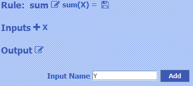 Figure 2
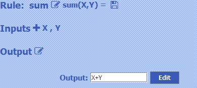 Figure 3
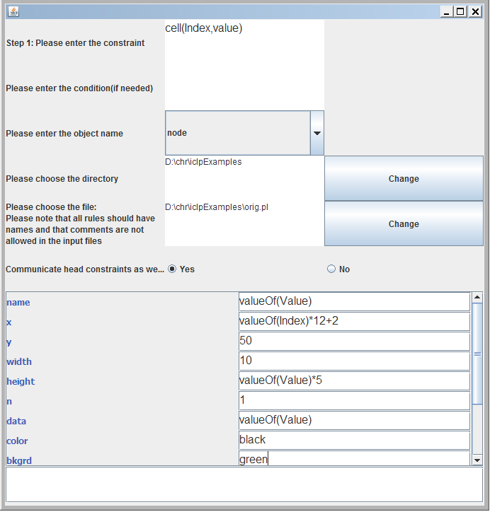 Figure 5
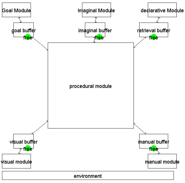 Figure 6
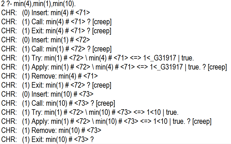 Figure 7
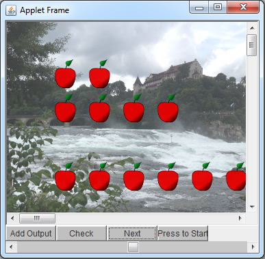 Figure 8
 Figure 9
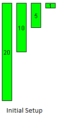 Figure 10
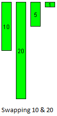 Figure 11
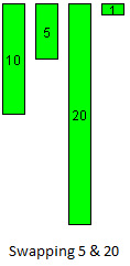 Figure 12
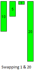 Figure 13
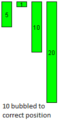 Figure 14
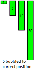 Figure 15
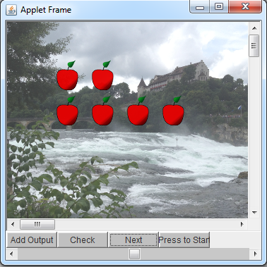 Figure 16
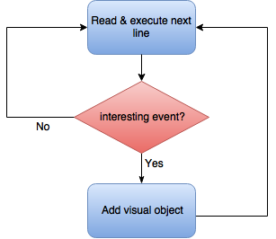 Figure 17
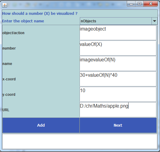 Figure 18
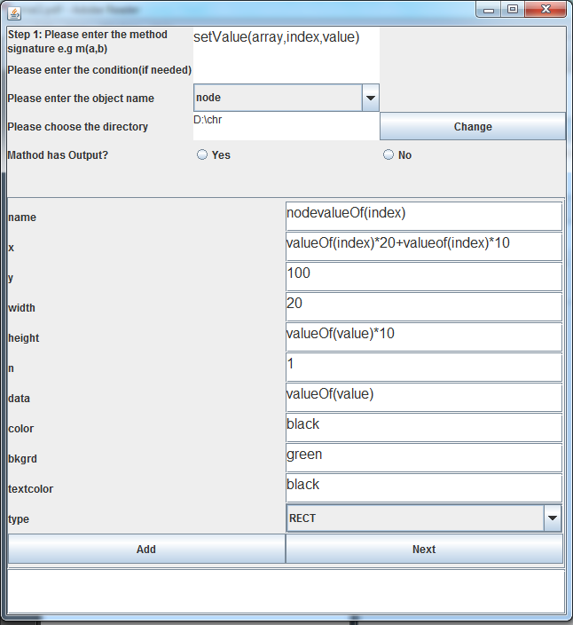 Figure 19
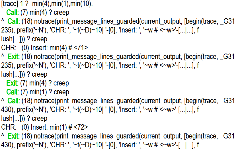 Figure 20
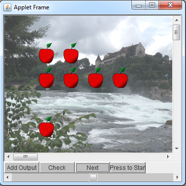 Figure 21
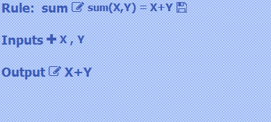 Figure 22
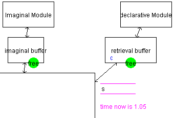 Figure 23
 Figure 24
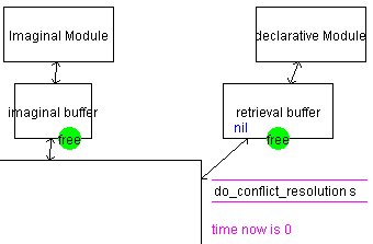 Figure 25
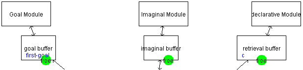 Figure 26
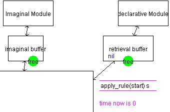 Figure 27
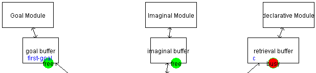 Figure 28
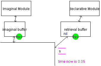 Figure 29
 Figure 30
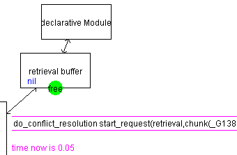 Figure 31
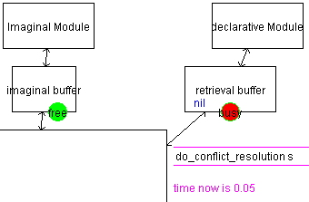 Figure 32
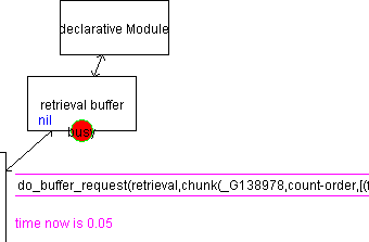 Figure 33
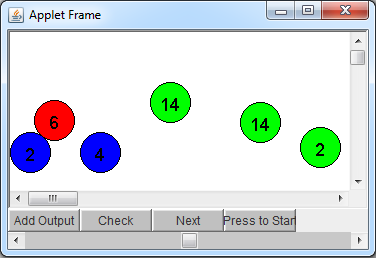 Figure 34
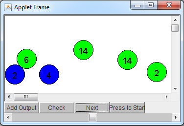 Figure 35
| 1. Solve : |
| given that is a built-in constraint and |
| 2. Introduce : |
| given that is a CHR constraint. |
| 3. Apply : |
| where there is a renamed rule in with variables with the form |
| such that |
| and |
| The constraint is introduced to the constraint store. | ||
| The constraint is introduced to the store. | ||
The rule remove_min is fired removing min(20) from the constraint store.
|
||
| The constraint is introduced to the store. | ||
The rule remove_min is fired removing min(8) from the constraint store.
|
| 1. Solve+wakeup : |
| given that is a built-in constraint and |
| and |
| 2. Activate |
| given that is a CHR constraint. |
| 3. Reactivate |
| given that is a CHR constraint. |
| 4. Apply |
| given that the jth occurrence of is part of the head of the re-named apart rule with variables : |
| where |
| and . |
| If occurs in then otherwise . |
| 5. Drop |
| given that is an occurrenced active constraint and has no occurrence in the program. |
| That could thus imply that all existing occurrences were tried before. |
| 6. Default |
| in case there is no other applicable transition. |
| The constraint is activated. | ||
| The active constraint did not fire any rule so the occurrence number is incremented. | ||
| The occurrence number is incremented. | ||
| The occurrence number is incremented. | ||
| The occurrence number is incremented. | ||
| The occurrence number is incremented. | ||
| The occurrence does not appear in the program. Thus, is dropped. | ||
| The occurrence does not appear in the program. Thus, is dropped. | ||
| The occurrence number is incremented. | ||
| The occurrence number is incremented. | ||
| The occurrence number is incremented. | ||
Rule remove_min is applied
|
||
| The occurrence number is incremented. | ||
| is dropped since the occurrence is never used in the program. | ||
| is activated. | ||
| The occurrence number is incremented. | ||
| The occurrence number is incremented. | ||
Rule remove_min is applied.
|
| 1. Solve+wakeup : |
| given that is a built-in constraint and |
| and |
| 2. Activate |
| given that is a CHR constraint. |
| 3. Reactivate |
| given that is a CHR constraint. |
| 4. Draw : |
| given that is a graphical object: . |
| and |
| The actual parameters of are used to visually render the object. |
| 5. Update Store : |
| given that is a graphical action: . |
| The actual parameters of are used to update the graphical objects. |
| 6. Apply_Annotation: |
| where there is: |
| a renamed, constraint annotation rule with variables of the form: |
| where is part of and |
| and |
| 7. Apply : |
| where: |
| • there is no applicable constraint annotation rule that involves . |
| (i.e. every applicable rule has already been applied). |
| In other words, for renamed-apart every annotation rule with variables : |
| , |
| is part of |
| It is already the case that: |
| • There is a renamed rule in with the form |
| with variables and the jth occurrence of is part of the head of the renamed rule, such that |
| where |
| and . |
| If occurs in then otherwise . |
If the program communicates the head constraints (i.e. contains comm_head(T) ==> T=true) then |
| 8. Drop |
| given that is an occurrenced active constraint and has no occurrence in the program |
| and that there is no applicable constraint annotation rule for the constraint . |
| That could thus imply that all existing ones were tried before. |
| 8. Default |
| in case there is no other applicable transition. |
| 1. Solve+wakeup: |
| given that is a built-in constraint and and |
| 2. Activate |
| given that is a CHR constraint. |
| 3. Reactivate |
| given that is a CHR constraint and is not a valid rule name. |
| 4. Draw : |
| given that is a graphical object: and |
| The actual parameters of are used to visually render the object. |
| 5. Update Store : |
| given that is a graphical action: . |
| The actual parameters of are used to update the graphical objects. |
| 6. Apply_Annotation: |
| where there is a, renamed, constraint annotation rule with variables of the form: |
| where is part of such that |
| and does not have an associated annotation rule and |
| 7. Apply : |
| there is and a renamed rule in with variables where the jth occurrence of is part of the head. |
| The renamed rule has the form: |
| such that )) |
| and and there are no associated and applicable annotation rule(s) to |
| or any part(s) of it that are not executed yet. |
| if and only if there is no annotation rule associated with |
| otherwise if has an associated rule under the same variables (matching) : |
| such that : |
| or |
| then |
| If occurs in then otherwise . |
If the program communicates the head constraints (i.e. contains comm_head(T) ==> T=true) then |
| otherwise . |
| 8. Drop |
| given that is an occurrenced active constraint and has no occurrence in the program |
| and that there is no applicable constraint annotation rule for the constraint c. |
| 9. Default |
| in case there is no other applicable transition. |
Peer Reviews
No public reviews on file for this paper yet. If you reviewed it on a platform where reviews are public (OpenReview, ICLR, NeurIPS, ICML), you can paste yours below so the community can read it here.
Videos
No videos yet. Explain this paper in a talk, walkthrough, or lecture? Add one.
Taxonomy
TopicsTeaching and Learning Programming · Model-Driven Software Engineering Techniques · Parallel Computing and Optimization Techniques
Visualization of Constraint Handling Rules: Semantics and Applications
Nada Sharaf
,
Slim Abdennadher
The German University in CairoComputer Science and EngineeringCairoEgypt
and
Thom Frühwirth
Ulm UniversityUlmGermany
Abstract.
The work in the paper presents an animation extension () to Constraint Handling Rules (CHR). Visualizations have always helped programmers understand data and debug programs. A picture is worth a thousand words. It can help identify where a problem is or show how something works. It can even illustrate a relation that was not clear otherwise. aims at embedding animation and visualization features into CHR programs. It thus enables users, while executing programs, to have such executions animated. The paper aims at providing the operational semantics for . The correctness of programs is also discussed. Some applications of the new extension are also introduced.
Constraint Handling Rules, Operational Semantics, Visualization, Animation
††journal: tocl††journalvolume: 9††journalnumber: 4††article: 39††journalyear: 2017††publicationmonth: 6††copyright: acmcopyright††doi: 0000001.0000001††ccs: Software and its engineering Constraint and logic languages ††ccs: Software and its engineering Visual language††ccs: Software and its engineering Integrated and visual development environments††ccs: Human-centered computing Information visualization††ccs: Human-centered computing Visualization theory, concepts and paradigms
1. Introduction
Animation tools are considered as a basic construct of programming languages. They are used to visualize the execution of a program. They provide users with a simple and intuitive method to debug and trace programs. This paper presents an extension to Constraint Handling Rules (CHR). The extension adds new visual features to CHR. It thus enables users to have executions of CHR programs animated.
CHR (Frühwirth, 2009, 1998) has evolved over the years into a general purpose language. Originally, it was proposed for writing constraint solvers. Due to its declarativity, it has, however, been used with different algorithms such as sorting algorithms, graph algorithms, … etc. CHR lacked tracing and debugging tools. Users were only able to use SWI-Prolog’s textual trace facility as shown in Figure 1 which is hard to follow especially with big programs.
Two types of visual facilities are important for a CHR programmer/beginner. Firstly, the programmer would like to get a visual trace showing which CHR rule gets applied at every step and its effect. Secondly, since CHR has developed into a general purpose language, it has been used with different types of algorithms such as sorting and graph algorithms. It is thus important to have a visual facility to animate the execution of the algorithms rather than just seeing the rules being executed. CHR lacked such a tool. The tool should be able to adapt with the execution nature of CHR programs where constraints are added and removed continuously from the constraint store.
Several approaches have been devised for visualizing CHR programs and its execution. In (Abdennadher and Saft, 2001), a tool called VisualCHR was proposed. VisualCHR allows its users to visually debug constraint solving. The compiler of JCHR (Schmauss, 1999) (on which VisualCHR is based) was modified. The visualization feature was thus not available for Prolog versions, the more prominent implementation of CHR. (Abdennadher and Sharaf, 2012) introduced a tool for visualizing the execution of CHR programs. It was able to show at every step the constraint store and the effect of applying each CHR rule in a step-by-step manner. The tool was based on the SWI-Prolog implementation of CHR. Source-to-source transformation was used in order to eliminate the need of doing any changes to the compiler. The tool could thus be deployed directly by any user. Source-to-source transformation is able to convert an original program automatically to a new one with the new features.
Despite of the availability of such visualization tools, CHR was still missing on a system for animating algorithms. The available tools were able to show at each point in time the executed rule and the status of the constraint store. However, the algorithm implemented had no effect on the produced visualization. Existing algorithm animation tools were either not generic enough or could not be adopted with CHR. For example, one of the available tools is XTANGO (Stasko, 1992) which is a general purpose animating system supporting the development of algorithm animations. However, the algorithm should be implemented in C or another language such that it produces a trace file to be read by a C program driver making it difficult to use with CHR. Due to the wide range of algorithms implemented through CHR, an algorithm-based animation was needed. Such animation should show at each step in time the changes to the data structure affected by the algorithm.
The paper presents a different direction for animating CHR programs. It allows users to animate any kind of algorithm implemented in CHR. This direction thus augments CHR with an animation extension. As a result, it allows a CHR programmer to trace the program from an algorithmic point of view independent of the details of the execution of its rules. The formal analysis of the new extension is presented in the paper. The paper thus presents a new operational semantics of CHR that embeds visualization into its execution. The formalism is able to capture not only the behavior of the CHR rules, it is also able to represent the graphical objects associated with the animation. It is used to prove the correctness of the programs extended with animation features. To eliminate the need of users learning the new syntax for using the extension, a transformation approach is also provided. The correctness of the transformation approach is presented in the paper too.
The paper is organized as follows: Section 2 introduces CHR. It starts with its syntax. It then shows two examples to show how CHR operates. The theoretical operational semantics is given in Section 2.2. The refined operational semantics is then introduced in Section 2.3. Section 3 introduces the new extension. The section starts by giving a general introduction. The syntax of annotation rules is then discussed and two examples are given. Finally, in Section 3.2 the formalization is given by introducing , a new operational semantics for CHR that accounts for annotation rules. The basic transitions include ones for simple constraint annotations. Afterwards, a more general semantics including rule annotations is presented. The separation was done to build the general semantics in an easy to follow method. Proofs of soundness and completeness are given. Section 4 presents a transformation approach that is able to transform normal CHR programs to programs. Section 5 introduces some applications that were built using . Conclusions and directions for future work are presented at the end of the paper.
2. Constraint Handling Rules
CHR was initially developed for writing constraint solvers (Frühwirth, 2009, 1998). The rules of a CHR program keeps on rewriting the constraints in the constraint store until a fixed point is reached. At that point no CHR rules could be applied. The constraint store is initialized by the constraints in the query of ths user. CHR has implementations in different languages such as Java, C and Haskell. The most prominent implementation, however, is the Prolog one. A CHR program has two types of constraints: user-defined/CHR constraints and built-in constraint. CHR constraints are defined by the user at the beginning of a program. Built-in constraints, on the other hand, are handled by (the constraint theory ) of the host language.
A CHR program consists of a set of, “simpagation rules". A simpagation rule has the following format:
optional_rule_name @ H_k \ H_r <=> G | B. and represent the head of the rule. The body of the rule is . The guard represents a precondition for applying the rule. A rule is only applied if the constraint store contains constraints that match the head of the rule and if the guard is satisfied. As seen from the previous rule, the head has two parts: and . The head of a rule could only contain CHR constraints. The guard should consist of built-in constraints. The body, on the other hand, can contain CHR and built-in constraints. On applying the rule, the constraints in are kept in the constraint store. The constraints in are removed from the constraint store. The body constraints are added to the constraint store.
There are two special kinds of CHR rules: propagation rules and simplification rules. A propagation rule has an empty thus such a rule does not remove any constraint from the constraint store. It has the following format:
optional_rule_name @ H_k ==> G | B.A simplification rule on the other hand has an empty . A simplification rule removes all the head constraints from the constraint store. A simplification rule has the following format:
optional_rule_name @ H_r <=> G | B.
2.1. Examples
This section introduces examples of CHR programs. Because of the declarativity of CHR and its rules, it is possible to implement different algorithms with single-ruled programs. The first program shows a sorting algorithm. The second program (consisting of two rules) aims at finding the minimum number out of a set of numbers.
2.1.1. Extracting the Minimum Number
The following program extracts the minimum number out of a set of numbers. Each number is represented by a min/1 The rule get_min is a simpagation CHR rule. It is applied whenever there are two numbers X and Y such that X is less than Y. The rule removes the bigger number, Y, from the constraint store. The smaller number, X, is kept in the constraint store. Thus, similar to the previous program, when the rule is no longer applicable, a fixed point is reached. By then, the constraint store would only contain the smallest number. The rule remove_dup is used to remove identical copies of the same number. The rule is thus fired if the user entered a sequence of numbers that contains duplicates.
:-chr_constraint min/1. remove_dup @ min(X) \ min(X) <> true. get_min @ min(X) \ min(Y) <=> X<Y | true.
The following example shows the steps taken to find the minimum number out of the set: 8, 3 and 1.
2.1.2. Sorting an Array
The program aims at sorting numbers in an array/list. Each number is represented by the constraint cell(I,V). I represents the index and V represents the value of the element. The program contains one rule: sort_rule. It is applied whenever the constraint store contains two cell constraints representing two unsorted elements. The guard makes sure that the two elements are not sorted with respect to each other. The element at index I1 has a value (V1) that is greater than the value (V2) of the element at index I2. I1 is less than I2. Thus, V1 precedes V2 in the array despite of the fact that it is greater than it. Since sort_rule is a simplification rule, the two constraints representing the unsorted elements are removed from the constraint store. Two cell constraints are added through the body of the rule to represent the performed swap to sort the two elements. The program is shown below:
:-chr_constraint cell/2. sort_rule @ cell(In1,V1), cell(In2,V2) <=> In1<In2,V1>V2 | cell(In2,V1), cell(In1,V2).
Successive applications of the rule makes sure that any two elements that are not sorted with respect to each other are swapped. The fixed point is reached whenever sort_rule is no longer applicable. At this point, the array is sorted.
The following shows how the query cell(0,7), cell(1,6), cell(2,4) affects the constraint store:111The examples in this section are running with the refined operational semantics explained later. For simplicity, Some details are omitted.
2.2. Theoretical Operational Semantics
A CHR state is represented by the tuple (Frühwirth, 2009; Betz et al., 2010). represents the goal store. It initially contains the query of the user. is the CHR constraint store containing the currently available CHR constraints. , on the other hand, is the built-in store with the built-ins handled by the host language (Prolog in this case). The propagation history, , holds the names of the applied CHR rules along with the IDs of the CHR constraints that activated the rules. is used to make sure a program does not run forever. Each CHR constraint is associated with an ID. represents the next available ID. represents the set of global variables. Such variables are the ones that exist in the initial query of the user. does not change during execution, it is thus omitted throughout the rest of the paper.
A variable is called a local variable (Raiser et al., 2009).
Definition 2.1.
The function chr is defined such that chr(c#n) = c. It is extended into sequences and sets of CHR constraints. Likewise, the function id is defined such that id(c#n) = n. It is also extended into sequences and sets of CHR constraints.
Definition 2.2.
denote the variables occurring in . denotes where vars(A) vars(F) = (Koninck et al., 2007; Duck et al., 2004a)
Table 1 shows the transitions of (from (Frühwirth, 2009)).The transitions are presented below:
Solve
The transition solve, adds the built-in constraint , in the goal store, to the built-in constraint store. The new built-in store is basically . The new store is also simplified.
Introduce
Similarly, Introduce, adds a CHR constraint () to the CHR constraint store. The ID of the constraint is . The next available ID is . The new CHR store is .
Apply
The Apply transition executes an available CHR rule r. When a rule is used, its variables are renamed apart from the program and the current state (Frühwirth, 2009). The fresh variant of the rule with variables the new variables : is executable under the applicability condition: . It first checks the built-in constraint store for satisfiablity. The rule is also only applied if the CHR constraint store contains matching constraints through the checks . Under the matching, the guard is also checked. It has to be logically entailed by the built-in constraints under the constraint theory (Frühwirth, 2009). To apply the rule, the propagation history should not contain a tuple representing the same constraints associated with the same rule signifying that this is the first time this rule is applied with those constraint(s). The constraints in the body are added to the goal. In addition, the propagation history is updated accordingly. Table 2 shows the query executed under for the program shown in Section 2.1.1.
2.3. Refined Operational Semantics
The refined operational semantics (Duck et al., 2004b; Frühwirth, 2009) is adapted in most implementations of CHR. It removes some of the sources of the non-determinism that exists in . In the order in which constraints are processed and the order of rule application in non-deterministic. However, in , rules are executed in a top-down manner. Thus, in the case where there are two matching rules , ensures that the rule that appears on top in the program is executed. Details of how works are shown in this section. Each atomic head constraint is associated with a number (occurrence). Numbering starts from . It follows a top-down approach as well. For example the previously shown program to find the minimum value is numbered as follows:
remove_dup @ min(X)_2\min(X)_1<=>true.
remove_min @ min(X)_4\min(Y)_3<=>X<Y | true.
Definition 2.3.
The active/occurrenced constraint c#i:j refers to a numbered constraint that should only match with occurrence j of the constraint c inside the program. is the identifier of the constraint (Duck et al., 2004b).
A state in is the tuple . Unlike , the goal is a stack instead of a multi-set. and have the same interpretation as an state. In the refined operational semantics, constraints are executed similar to procedure calls. Each constraint added to the store is activated. An active constraint searches for an applicable rule. The rule search is done in a top-down approach. If a rule matches, the newly added constraints (from the body of the applied rule) could in turn fire new rules. Once all rules are fired, execution resumes from the same point. Constraints in the constraint store are reconsidered/woken if a newly added built-in constraint could affect them (according to the wakeup policy). An active constraint thus tries to match with all the rules in the program
Table 3 shows the transitions of .
2.3.1. Solve+Wake
This transition introduces a built-in constraint to the built-in store. In addition, all constraints that could be affected by () are woken up by adding them on top of the stack. These constraints are thus re-activated. A constraint where all its terms have become ground will not be thus woken up by the implemented wake-up policy since it is never affected by a new built-in constraint. where represents the variables fixed by .
2.3.2. Activate
This transition introduces a CHR constraint into the constraint store and activates it. The introduced constraint has the occurrence value as a start.
2.3.3. Reactivate
The reactivate transition considers a constraint that was already added to the store before. It became re-activated and was added to the stack. The transition activates the constraint by associating it with an occurrence value starting with .
2.3.4. Apply
This transition applies a CHR rule if an active constraint matched a constraint in the head of with the same occurrence number. If the matched constraint is part of the constraints to be removed, it is also removed from the stack. Otherwise, it is kept in the constraint store and the stack.
2.3.5. Drop
This transition removes the active constraint from the stack when there no more occurrences to check. This occurs when the occurrence number of the active constraint does not appear in the program. In other words, the existing ones were tried.
2.3.6. Default
This transition proceeds to the next occurrence of the constraint if the currently active one could not be matched with the associated rule. This transition ensures that all occurrences are tried.
2.3.7. Running Example
In the beginning of the section, a CHR program to find the minimum number among a set of numbers was given. The program was written with the numbered constraint occurrences as used by . For the query min(20),min(1),min(8), the steps shown in Table 4 take place.
3. : An Animation Extension for CHR
The proposed extension aims at embedding visualization and animation features into CHR programs. The basic idea is that some constraints, the interesting ones, are annotated by visual objects. Thus on adding (removing) such constraints to (from) the constraint store, the corresponding graphical object is added (removed) to (from) the graphical store. These constraints are thus treated as interesting events. Interesting constraints are those constraints that directly represent/affect the basic data structure used along the program. Visualizing such constraints thus leads to a visualization of the execution of the corresponding program. In addition, changes in the constraint store affects the data structure and its visualization. This results in an animation of the execution. For example, in a program to encode the “Sudoku” game, the interesting constraints would be those representing the different cells in the board and their values. Another example is a program solving the -queens problem. The program aims at placing queens on an board so that the queens cannot attack each other horizontally, vertically or diagonally. In this case, the interesting constraints are those reflecting the board and the current/possible locations for each of the queens (Sharaf et al., 2014b, a).
The approach aims at introducing a generic animation platform independent of the implemented algorithm. This is achieved through two features. First, annotation rules are used. The idea of using interesting events for animating programs was introduced before in Balsa (Brown and Sedgewick, 1984) and Zeus (Brown, 1991). Both system use the notion of interesting events. However, users need to know many details to be able to use them. However, eliminated the need of the user knowing any details about the animation. The second feature is outsourcing the animation into an existing visual tool. For proof of concept, Jawaa (Pierson and Rodger, 1998), was used. Jawaa provides its users with a wide range of basic structures such as a circle, rectangle, line, textual node , … etc. Users can also apply actions on Jawaa objects such as movement, changing a color , … etc. Users are able to write their own programs with the syntax discussed later in this section. However, users are also provided with an interface (as shown in Figure 2) that allows them to specify every interesting event/constraint. In that case, the programs are automatically generated.
They are then able to choose the visual object/action (from the list of Jawaa objects/actions) to link the constraint to. Once they make a choice, the panel is populated with the corresponding parameters. Parameters represent the visual properties of the object such as: color, x-coordinate, … etc. Users have to specify a value for each parameter. A value could be:
- (1)
a constant value e.g. 100, blue, … etc. 2. (2)
the function valueOf/1. valueOf(X) outputs the value of the argument X such that X is one of the arguments of the interesting constraint. 3. (3)
the function prologValue/1. prologValue(Exp) outputs the value of the argument “X” computed through the mathematical expression Exp. 4. (4)
The keyword random that generates a random number.
3.1. Extended Programs
This section introduces the syntax of the CHR programs that are able to produce animations on execution. In addition to the basic constructs of a CHR program, the extended version needs to specify:
- (1)
The graphical objects to be used throughout the programs. 2. (2)
The interesting constraints and their association with graphical objects. 3. (3)
Whether the head constraints are to be communicated to the tracer.
In case, the head constraints are communicated, every time a constraint is removed from the store, its
associated visual object is also removed. In some of the cases, this will not be necessary as seen in the below
examples.
3.1.1. Syntax of
The annotation rules that associate CHR constraint(s) with objects have the following format:
[TABLE]
contains either one interesting constraint or a group of interesting constraints that are associated with a graphical object. Similar to normal CHR rules, graphical annotation rules could have a pre-condition that has to be satisfied for the rule to be applied. The literal is added at the beginning of the rule to differentiate between CHR and annotation rules. A program thus has two types of rules. There are the normal CHR rules and the annotation rules responsible for associating CHR constraint(s) with graphical object(s). Moreover there are meta-annotation rules that associate CHR rules with graphical object(s). In this case, instead of associating CHR constraint(s) with visual object(s), the association is for a CHR rule. In other words, once such rule is executed the associated visual objects are produced. The association is thus done with the execution of the rule rather than the generation of a new CHR constraint. The rule annotation is done through associating a rule with an auxiliary constraint. The auxiliary constraint has a normal constraint annotation rule with the required visual object. Such meta-annotation rule has the following format:
[TABLE]
[TABLE]
In addition, a rule for comm_head/1 has to be added in the program.
(comm_head(T) ==> T=true.) means that head constraints are to be communicated to the tracer.
(comm_head(T) ==> T=false.) means that the removed head constraints should not affect the visualization.
3.1.2. Examples
The program provided in Section 2.1.2 aims at sorting an array of numbers. In order to animate the execution, we need to visualize the elements of the array. Changes of the elements lead to a change in the visualization and thus animating the algorithm. The interesting constraint in this case is the cell constraint. As shown in Figure 2, it was associated with a rectangular node whose height is a factor of the value of the element. The x-coordinate is a factor of the index. That way, the location and size of a node represent an element of the array.
The new program is:
:-chr_constraint cell/2.:-chr_constraint comm_head/1.comm_head(T) ==> T=true.sort_rule @ cell(In1,V1), cell(In2,V2) <=> In1<In2,V1>V2 | cell(In2,V1), cell(In1,V2).g ann_rule_cell cell(Index,Value) ==> node(valueOf(Value),valueOf(Index)*12+2, 50,10,valueOf(Value)*5 ,1,valueOf(Value), black, green, black, RECT).Figure 3b shows the result of running the query cell(0,7),cell(1,6),cell(2,4). As shown from the taken steps, each number added to the array and thus to the constraint store adds a corresponding rectangular node. Once cell(0,7) and cell(1,6) are added to the constraint store, the rule sort_rule is applicable. Thus, the two constraints are removed from the store. The rule adds cell(1,7) and cell(0,6) to the constraint store.
Afterwards, cell(2,4) is added to the store. At this point cell(0,6) and cell(2,4) activate sort_rule and are removed from the constraint store. The rule first adds cell(2,6) to the store. At this point cell(1,7) and cell(2,6) activate sort_rule again. Thus they are both removed from the store. The constraints cell(2,7), cell(1,6) are added. Afterwards, the last constraint cell(0,4) is added to the store. As seen from Figure 3b, using annotations for constraints has helped animate the execution of the sorting algorithm. However, in some of the steps, it might not have been clear which two numbers are being swapped. In that case it would be useful to use an annotation for the rule sort_rule instead of only annotating the constraint list. The resulting program looks as follows:
:-chr_constraint cell/2.:-chr_constraint comm_head/1.comm_head(T) ==> T=false.sort_rule @ cell(In1,V1), cell(In2,V2) <=> In1<In2,V1>V2 | cell(In2,V1), cell(In1,V2), swap(In1,V1,In2,V2).g ann_rule_cell cell(Index,Value) ==> node(nodevalueOf(Value),valueOf(Index)*12+2,50,10, valueOf(Value)*5 , 1, valueOf(Value), black, green, black, RECT).g swap(In1,V1,In2,V2) ==> changeParam(nodevalueOf(V1),bkgrd,pink)g swap(In1,V1,In2,V2) ==> changeParam(nodevalueOf(V2),bkgrd,pink)g swap(In1,V1,In2,V2) ==> moveRelative(nodevalueOf(V1), (valueOf(I2)-valueOf(I1))12,0)g swap(In1,V1,In2,V2) ==> moveRelative(nodevalueOf(V2), (valueOf(I2)-valueOf(I1))(-12),0)g swap(In1,V1,In2,V2) ==> changeParam(nodevalueOf(V1),bkgrd,green)g swap(In1,V1,In2,V2) ==> changeParam(nodevalueOf(V2),bkgrd,green)g sort_rule ==> swap(In1,V1,In2,V2).The annotations make sure that once two numbers are swapped, they are first marked with a different color (pink in this case). The two rectangular bars are then moved. The bar on the left is moved to the right. The bar on the right is moved to the left (negative displacement). The space between the start of one node and the start of the next node is 12 pixels. Thus the displacement is calculated as the difference between the two indeces multiplied by 12. After the swap is done, the two bars are colored back into green. The result of executing the query: cell(0,7),cell(1,6),cell(2,4) is shown in Figure 4c.
3.2. Animation Formalization
The rest of the section offers a formalization of the animation to be able to run programs and reason about their correctness. The basic idea is introducing a new “graphical" store. adds, besides the classical constraint store of CHR, a new store called the graphical store. As implied by the name, the graphical store contains graphical/visual objects. Such objects are the visual mappings of the interesting constraints. Over the course of the program execution, and as a result of applying the different rules, the constraint store as well as the graphical store change. As introduced before, the change of the visual objects leads to an animation of the program.
Definition 3.1.
In , a state is represented by a tuple . , , , , and have the same meanings as in a normal CHR state (goal store, CHR constraint store, built-in store, propagation history and the next available identification number). is a store of graphical objects. is the history of the applications of the visual annotation rules. Each element in has the following format: where
- •
represents the name of the fired annotation rule.
- •
contain the ids of the head constraints that fired the annotation rule.
- •
are the ids of the graphical objects added to the graphical store through firing using .
Definition 3.2.
For a sequence , the function .
Definition 3.3.
Two sequences and are equivalent: if
- (1)
For every , if exists times in such that , then exists times in . 2. (2)
For every , if exists times in such that , then exists times in .
Definition 3.4.
The function such that:
- •
.
- •
Each parameter such that
- –
if is a constant value then .
- –
if then .
- –
if then where is evaluated in SWI-Prolog and binds the variable to a value.
- –
if , then is a randomly computed number.
Definition 3.5.
The function
[TABLE]
Any could have a different graphical aspect such as its color, x-coordinate, … etc.
Definition 3.6.
The function such that: in the case where ,
,
Definition 3.7.
The function such that: in the case where
,
.
Definition 3.8.
The function is:
- •
in the case where contains a tuple of the form .
- •
in the case where does not contain a tuple of the form .
Table LABEL:table:omegavis shows the basic transitions of . To make the transitions easier to follow, table LABEL:table:omegavis shows the transitions needed to run CHR programs with constraint annotation rules. Annotations of CHR rules are thus discarded from the first set of transitions. allows for running programs that contain constraint annotations. The three transitions and are responsible for dealing with the graphical store and its constituents. The transition, , applies a constraint annotation rule. The rest of the transitions, such as solve, introduce and apply, have the same behavior as in . These transitions do not affect the graphical store or the application history of the annotation rules.
The transitions affecting the graphical store are:
- (1)
Draw
The new transition draw adds a graphical object () to the graphical store. Since multiple copies of a graphical object are allowed, each object is associated with a unique identifier. 2. (2)
Apply_Annotation
The Apply_Annotation transition applies a constraint annotation rule (ann_rule). An annotation rule is applicable if the CHR constraint store contains matching constraints. The condition of the rule has to be implied by the built in store under the matching. The built in constraint store B is also first checked for satisfiability. For the rule to be applied, it should not have appeared in the history of applied annotation rules with the same constraints i.e. it should be the first time the constraint(s) fire this annotation rule. Executing the rule adds to the goal the graphical object in the body of the executed annotation rule. The history of annotation rules is updated accordingly with the name of the rule in addition to the id(s) of the CHR constraint(s) in the head. In fact, this transition has a higher precedence than the transition . Thus in the case where an annotation rule and a CHR rule are applicable, the annotation rule is triggered first.The precedence makes sure that graphical objects are added in the intended order. This ensures producing correct animations.
Definition 3.9 (Built-In Store Equivalence).
Two built-in constraint stores and are considered equivalent iff:
where and are the local variables inside and respectively. The equivalence thus basically ensures that there are no contradictions in the substitutions since local variables are renamed apart in every CHR program. The equivalence check thus ensures the logical equivalence rather than the syntactical equivalence.
Definition 3.10.
A state is equivalent to a CHR state if and only if
- (1)
according to Definition 3.3. 2. (2)
according to Definition 3.3. 3. (3)
and are equivalent according to Definition 3.9. 4. (4)
5. (5)
The idea is that a state basically has an extra graphical store. The correspondence check is effectively done through the CHR constraints since they are the most distinguishing constituents of a state. Thus, the constraint store and the stack should contain the same constraints. The propagation history should be also the same indicating that the same CHR rules have been applied. could, however, have a value higher than . This is due to the fact that graphical objects have identifiers.
The definition of state equivalence described here follows the properties introduced in (Raiser et al., 2009). However, it is stricter.
Theorem 3.11 (Completeness).
Given a CHR program (running under ) along with its user defined annotations and its corresponding (running under ) program, for the same query , every derived state : has an equivalent state : .
Proof.
Base Case: For a given query , the initial state in . The initial state in is .222Throughout the different proofs, identifiers are omitted for brevity According to Definition 3.10 and are equivalent.
Induction Hypothesis: Suppose that there are two equivalent derived states and such that and .
Induction Step: According to the induction hypothesis, and are equivalent. The rest of the proof shows that any transition applicable to in produces a state that has an equivalent state produced by applying a transition to in . Thus, no matter how many times the step is repeated, the output states are equivalent.
- •
Case 1: (Applying Solve+wakeup):
In this case, such that:
Transition solve+wakeup is applicable if:
- (1)
is a built-in constraint 2. (2)
3. (3)
is equivalent to . Thus according to Definition 3.10, Thus accordingly, the transition is applicable to under producing :. According to Definition 3.10, is equivalent to
- •
Case 2: (Applying Activate):
In this case, where is a CHR constraint. Thus .
Since is equivalent to . Thus according to Definition 3.10:
Accordingly, which is equivalent to . (Since , then ).
- •
Case 3 (Applying Reactivate):
The transition reactivate is applicable if the stack has on top of it an element of the form where is a CHR constraint. In this case . Accordingly, . Since and are equivalent, then has the same stack. triggers the transition reactivate producing which is also equivalent to . Since is not associated with an occurrence yet, no annotation rule is applicable at this point.
- •
Case 4: (Applying the transition Apply)
The transition Apply is triggered under in the case where such that the jth occurrence of is part of the head of the re-named apart rule with variables :
such that:
and .
Thus in such a case
[TABLE]
Due to the fact that and are equivalent, in the case where triggers the transition Apply under , the same rule is also applicable under to . However for , one of two possibilities could happen:
• There is no applicable constraint annotation rule:
This could be due to the fact that any applicable annotation rule was already executed or that there re no applicable annotation rules at this point. In this case,the transition is triggered right away under producing a state
(
) equivalent to ().
The original states are equivalent and the same rule is applied in both cases. We can assume that, without loss of generality , in the program, the rule is renamed using the same variables resulting in the same matching. This is because the same matching should happen to be able to apply the same rule using the given constraint stores.
• There is an applicable annotation rule:
In this case an annotation rule () for is applicable such that:
according to the previously mentioned conditions.
At this point either the transition Draw or Update store is applicable such that:
S_{chr_{vis}}^{\prime}\mapsto_{draw\big{/}updatestore}S_{chr_{vis}}^{\prime\prime}:\langle\left[c\#i:j|A\right],H_{1}\uplus H_{2}\uplus S,Gr^{\prime},B,
In case is a graphical object, the transition Draw is applied such that: .
In case, is a graphical action, the transition Update Store is applied such that:
Since the two transitions, could only change the graphical stores, annotation history and the next available identifier, the equivalence of the states is not affected.
At this point fires the transition for the same CHR rule that triggered the same transition under earlier. The produced state has the format:
.
Similarly the same matching (local variable renaming ) has to be applied for the rule to fire.
Consequently, according to Definition 3.10, the state is still equivalent to
- •
Case 5: Applying the transition Drop
In the case where the top of the stack has an occurrenced active constraint such that has no occurrence in the program, the transition drop is applied. Thus,
Since and are equivalent, the stack of both states have to be equivalent.
Thus . For one of two possibilities is applicable:
- (1)
No annotation rule is applicable. This could be either because is not associated with any visual annotation rules or because all such rules have been already applied. In this case
2. (2)
The second possibility is the existence of an applicable annotation rule: transforming to . At that point either draw or update store are to be applied transforming to
. At that point, the transition drop is applicable converting to . is equivalent to
- •
Case 6: Applying the Default Transition
If none of the previous cases is applicable,
For the equivalent , one of two possible cases could happen:
- (1)
Apply annotation is not applicable:
In that case, the Default transition is directly applied transforming such that
.
The produced state () is equivalent to as well. 2. (2)
Apply annotation is applicable:
In this case an annotation rule for one of the existing constraints is applicable such that:
according to the previously mentioned conditions.
At this point either the transition Draw or the transition Update store is applicable such that:
is still equivalent to .
At the point where the transition apply_annotation is no longer applicable, the only applicable transition is Default transforming to such that . According to Definition 3.10, is equivalent to
Thus in all cases an equivalent state is produced under ∎
∎
Theorem 3.12 (Soundness).
Given a CHR program (running under ) along with its user defined annotations and its corresponding program (running under ), for the same query , every derived state : has en equivalent state :
Proof.
Base Case:
For the initial query the two states , and are equivalent according to Definition 3.10.
Induction Hypothesis: Suppose that there are two equivalent derived states and such that and .
Induction Step:
The proof shows that any transition applicable to under produces a state such that under applying a transition to (which is equivalent to ) produces a state that is equivalent to .
The different cases are enumerated below:
- (1)
Case 1: Applying solve+wakeup to :
Under , solve+wakeup is applicable in the case where the stack has the form such that c is a built-in constraint and
and such that
. Since and are equivalent, has an equivalent stack and built-in store according to Definition 3.10. Thus the corresponding transition solve+wakeup is applicable to under producing a state such that: . According to Definition 3.10, the two states and are equivalent. 2. (2)
Case 2: Applying Activate:
Such a transition is applicable to under in the case where the top of the stack of contains a CHR constraint . In this case:
given that is a CHR constraint.
The equivalent state has the same stack triggering the transition Activate under producing a state which is also equivalent to 3. (3)
Case 3: Applying Reactivate:
In this case,
such that and is a CHR constraint.
The equivalent state has an equivalent stack triggering the transition reactivate under . The transition application produces which is also equivalent to . 4. (4)
According to Definition 3.10 and since is equivalent to , they both have the same stack. The transition Draw is only applicable if the top of the stack contains a graphical object. Since the stack of never contains graphical objects and since it is equivalent to , the stack of at this point does not contain graphical objects as well. Thus, in this case, the transition Draw is not applicable to under . 5. (5)
Similarly, according to Definition 3.10 and since is equivalent to , the stack of at this point does not contain graphical actions since both states should have the same stack. The transition Update store is only applicable if the top of the stack contains a graphical action. Thus, in this case, the transition Update store is not applicable to under . 6. (6)
Case 4: Apply Annotation Rule Transition
The transition Apply Annotation is triggered when the stack has on top a constraint associated with an annotation rule. The constraint store should contain constraints matching the head of the annotation rule such that this rule was not fired with those constraint(s) before and the pre-condition of the annotation rule is satisfied. Thus, the rule could be associated with more than one constraint including the one on top of the stack.
The constraint store should however, contain matching constraints for the rest of the constraints in the head of
the annotation rule.
such that . The renamed annotation rule with variables is :
Either the transition Draw or Update store is applicable to . The output is . In case, is a graphical object, then . In case, is a graphical action, then Any transition applicable to at this stage is covered through the rest of the cases. Thus the application of the transition is considered as not to affect the equivalence of the output state with . 7. (7)
Case 5: the Apply transition
In the case where a CHR rule is applicable to , the transition Apply is triggered under . A CHR rule is applicable in the case where a renamed version of the rule with variables : () where and . In this case, has the form: . The output state has the form
. Due to the fact that is equivalent to ,it has the following form: . For the same program, the CHR rule is applicable producing :
[TABLE]
Due to the fact that the same CHR rule is applied for both states, the new built-in stores are equivalent according to Definition 3.9. This is due to the fact that since the original states have equivalent constraint stores, we assume without loss of generality that the matchings in both cases are the same since the same rule was applied. Thus, the rule in the two programs and are renamed similarly.
At this point, for one of two cases is possible:
- •
An annotation rule is applicable:
In this case, has the form where there exists a renamed, constraint annotation rule with the same variables of the form: where is part of
such that and . The output state has the form:
.
Similar to the previous cases, triggers the transition draw or update store producing . According to Definition 3.10, is equivalent to since the two stacks, constraint stores and propagation histories are not affected by the application of the annotation rule.
- •
No annotation rule is applicable
At this point, is still equivalent to 8. (8)
Case 6: Applying Drop
In the case where such that has no occurrence in the program and case 5 is not applicable, the transition Drop is triggered. Drop produces the state
given that is an occurrenced active constraint and has no occurrence in the program.
Since is equivalent to , they both have the same stack . Thus under , the same transition drop is triggered producing . According to Definition 3.10, and are equivalent as well. 9. (9)
Case 7: Applying Default
In the case where none of the above cases hold, the transition Default transforms to
. Similarly the equivalent state triggers the same transition Default in this case. The output state is still equivalent to
∎
3.2.1. Operational Semantics including Rule Annotations
Table LABEL:table:omegavisruleann shows the operational semantics of . is basically but taking rule annotations into account. A state of is a tuple . , , , , , , and have the same meanings as in an state. However, can hold ,in addition to the previously seen formats of constraints, the constraint in addition the name of the rule that added it. holds for each constraint, its ID in addition to the name of the rule used to add it. It is an extended form of the constraint store. If the constraint comes from the query of the user or if it is an auxiliary constraint, the keyword, aux is used for the rule name inside and .
Definition 3.13.
Similar to the previously defined functions, for a state , is a function defined as: such that
Definition 3.14.
The definition of the function is modified such that: for a sequence the function such that is not an auxiliary constraint. could thus represent identifiers or rule names. Definition 3.14 is thus reflected in the equivalence definition of states introduced in Definition 3.10
As seen through Table LABEL:table:omegavisruleann, the transition Apply could activate a rule annotation (if applicable) associated with the applied CHR rule. In this case, the auxiliary constraint is added to the goal with the keyword . Since the CHR rule is applied with the combination of constraints once, the rule annotation is also applied once and there is no risk of running infinitely. The rest of the transitions were modified only to include the newly added state parameter . In addition, the apply annotation transition is only applied if the constraints activating it were not added by a rule that is associated with a rule annotation rule. This ensures the previously discussed property that whenever a rule is associated with a rule annotation, then the body constraints can never trigger their own visual annotation rules. Since the rule is annotated then the individual constraint annotations are discarded.
3.2.2. Completeness and Soundness
Since according to the modified definition shown in Definition 3.14, the state equivalence will not take auxiliary constraints into account. The proofs for completeness and soundness shown in Proof 3.11 and Proof 3.12 still hold. As seen from the transitions in Table LABEL:table:omegavisruleann, the auxiliary constraint of the rule annotation is dealt with as a normal CHR constraint. Thus the only difference between these transitions and the previous ones is that sometimes, auxiliary constraints will exist in the constraint store of the final states. The states however remain equivalent. Thus even if annotations of rules were applicable, is still sound and complete.
Proof 3.11 introduced for the completeness check has the following amendment in the induction step:
Case 4: (Applying the transition Apply)
For , the transition Apply is triggered in the case where such that the jth occurrence of is part of the head of the re-named apart rule with variables :
and . In this case,
[TABLE]
Due to the fact that and are equivalent, they both have the same goal stacks and constraint stores. However for one of two possibilities could take place.
• It could be that there is no applicable constraint constraint annotation rule either because any applicable annotation rule was already executed or at this point there is no applicable annotation rule at this point. The transition is thus triggered right away under .
• It could, however, be the case that there is an applicable constraint annotation rule.
In this case an annotation rule () for is applicable such that:
.
At this point either the transition Draw or Update store should be applied. Thus,
S_{chr_{vis}}^{\prime}\mapsto_{draw\big{/}updatestore}S_{chr_{vis}}^{\prime}:\langle\left[c\#i:j|A\right],H_{1}\uplus H_{2}\uplus S,Gr^{\prime},B,
The transition Draw is applicable in case is a graphical object such that: .
In the case where is a graphical action, the transition Update Store is applied such that:
The two transitions do not affect the constraint stores or goal stacks. Thus, the equivalence of the states is not affected.
Due to the fact that and are equivalent, in the case where triggers the transition Apply under , also triggers the same transition for the same CHR rule, under producing a state ( ) where
and
[TABLE]
Since the same rule is applied in both cases, the two resulting states and () are equivalent. Similarly, the matchings in both cases are have to be the same since the original states have equivalent stores. Thus. without loss of generality, the applied rule is assumed to be renamed with the same variables in both programs. The two new built-in stores are still equivalent and the two resulting states are thus also equivalent.
If the program communicates the head constraints (i.e. contains comm_head(T) ==> T=true) then
There are however, two possibilities in this case,
- •
if is associated with an annotation rule (renamed with variables )
.
where
In this case, .
is thus still equivalent to since auxiliary constraints are disregarded in the equality check.
- •
if is not associated with an annotation or if the annotation is not applicable then making the two states and equivalent as well.
As for the soundness proof (Proof 3.12), the only change is in the following case:
Case 5: the Apply transition
In the case where a CHR rule is applicable to , the transition Apply is triggered under . A CHR rule is applicable in the case where a renamed version of the rule with variables is
() where and
. In this case, has the form: . The output state has the form
. Due to the fact that is equivalent to ,it has the following form: . For the same program, the CHR rule is applicable producing :
such that
. Similarly, without loss of generarility the same variable renaming was used for both programs. Thus, the two new built-in stores are equivalent according to Definition 3.9 since only one possible matching would be possible since the original two states have equivalent stores. Moreover,
[TABLE]
. In addition,
[TABLE]
. If a rule annotation () is applicable, then where otherwise .
In both cases, the output states are still equivalent since the equivalence check neglects auxiliary constraints and the graphical store.
4. to Transformation Approach
The aim of the transformation is to eliminate the need of doing any compiler modifications in order to animate CHR programs. A program is thus transformed to a corresponding program with the same behavior. is thus able to produce the same states in terms of CHR constraints and visual objects as well.
As a first step, the transformation adds for every constraint constraint/n a rule of the form:
The extra rule ensures that every time a constraint is added to the store, the tracer (external module) is notified. If constraint was annotated as an interesting constraint, its corresponding annotation rule is activated producing the corresponding visual object(s). The new rules communicate any constraint added to the constraint store.
The user can also choose to communicate to the tracer the head constraints since they could affect the animation. A removed head constraint could affect the visualization in case it is an interesting constraint. In this case, if the user chose to communicate head constraints, the associated visual object, produced before, should be removed from the visual trace.333The tracer is able to handle the problem of having multiple Jawaa objects with the same name by removing the old object having the same name before adding the new one. This is possible even if the removed head constraint was not communicated..
As a second step, the transformer adds for every compound constraint-annotation of the form:
, a new rule of the form:
.
By default, a propagation rule is produced to keep in the constraint store. However, the transformer could be instructed to produce a simplification rule instead. The annotation is triggered whenever exist in the constraint store. Whenever this is the case, the rule is triggered producing the annotation constraint. Since the annotation constraint is a normal CHR constraint, it is automatically communicated to the tracer using the previous step.
As a third step, the CHR rules annotated by the user as interesting rules should be transformed. The idea is that the CHR constraints produced by such rules should be ignored. In other words, even if the rule produces an interesting CHR constraint, it should not trigger the corresponding constraint annotation. Instead, the rule annotation is triggered.
Hence, to avoid having problems with this case, a generic status is used throughout the transformed program . Any rule annotated by the user as an interesting rule changes the status to at execution. However, the rules added in the previous two steps check that the status is set to . In other words, if the interesting rule is triggered, no constraint is communicated to the tracer since the guard of the corresponding rule fails. Any rule with the corresponding annotation is transformed to: In addition, the transformer adds the following rule to :
.
The new rule thus ensures that the events associated with the rule annotation are considered and that all annotations associated with the constraints in the body of the rule are ignored.
4.1. Correctness of Transformation Approach
The aim of the transformation process is to produce a program () that is able to perform the same behavior of the corresponding program () which basically contains the original CHR program along with the constraint(s) and rule annotations. This section shows that the transformed program, using the steps shown previously, is a correct one. In other words, for the same query , produces an equivalent state to the one produced by . As seen from the previous section was proven to be sound and complete. This implies that any state reachable by is also reachable by . In addition, any state reachable by is also reachable by . The focus of this section is the initial CHR program provided by the user. The aim is to make sure that produces the same CHR constraints that produces to make sure that the transformation did not change the behavior that was initially intended by the programmer. The focus is thus to compare how and perform over .
Theorem 4.1.
*Given a CHR program (along with its annotations) and its corresponding transformed program and two states and where contains the initial goal constraints and is a set of auxiliary constraints. Then the following holds:
If and then is equivalent to *
Proof.
(Sketch) The below sketch shows how the constraint store changes over the course of running the same query in and .
Executing a query in takes the following steps. The store at each step starts with the final value of the previous one
- (1)
Step 1: The constraint store of () start off by being empty (). . 2. (2)
Step2: The constraints in the query start to get activated and enter the constraint store . starts off by being equal to . Every time a constraint gets activated, it enters the store converting to . 3. (3)
Step 3: Applying a rule , adds to . The components of are also removed from it. Thus after the rule application, . 4. (4)
Step 4: Go Back to step 3. Any applicable rule is fired changing the constraint store. Step 3 keeps on repeating until no more rules are applicable reaching a fixed point.
In executing the same query undergoes the following steps. Similarly, the store at each step starts with the final value of the previous one
- (1)
Step 1: Initially the constraints store is also empty. Thus, . 2. (2)
Step 2: The query constraints start to get activated and enter the constraint store . starts off by being equal to . When a constraint gets activated, it enters the store. thus is augmented with and the result is . 3. (3)
Step 3: In , each time a constraint gets activated and enters the store, the corresponding rule: is triggered. is a propagation rule. Thus it does not remove any constraint from the store. The body of the rule communicates the constraint to the tracer, not adding anything to the store as well. At this point . 4. (4)
Step 4 (Optional): In , if there are any compound annotations for constraints () in , the corresponding rule is fired adding to the the auxiliary constraint:
.
fires the corresponding rule. Thus, where . 5. (5)
Step 5: contains the same CHR rules as in . Consequently, whenever a rule is applicable in , the same rule will be also applicable in . Applying a rule , adds to . The components of are also removed from the store. Thus after the rule application, . In case has an associated annotation rule, Once the constraints in are added to the store, the corresponding rules are matched. However, since their guard fails (as the status is set to true in , the rules do not file. In case has an associated annotation rule, the auxiliary constraint is added to the store. Afterwards, triggers the simplification rule communicating the constraint to the tracer. Since the rule is a simplification rule, is then removed from the constraint store keeping . 6. (6)
Step 3 and 4 could be applied for the new constraint store. As sen previously, step 3 does not change the constraint store. Step 4 could however add some auxiliary constraints to .
∎
As seen before, in all the previous steps, either or where contains some extra auxiliary constraints. Thus, the transformation does not change in the intended application of .
5. Applications
This section introduces different applications of the proposed semantics. The applications cover different fields were animations were useful.
5.1. Animating Java Programs
The idea of annotating constraints with visual objects was extended to Java programs in (Sharaf et al., 2016a). The execution path of the new programs is shown in Figure 5.
Using visual annotation rules of CHR programs, Java programs could also be animated in a generic way. The objective is to annotate method calls as interesting events. They are thus linked with visual objects. Thus, every time a method is invoked, its corresponding visual object is added. This results in animating the algorithm while it is running. That way, the user does not have to get into any of the technical details of how the visualization is produced. They only need to state what they want to see.
For every interesting method , one CHR rule is produced. The rule simply communicates the fact the the method with the arguments was called in the Java program. The rule has the following format:
m(arg_1,...,arg_n) ==> communicate_event(m(arg_1,...,arg_n)).
For example, the below Java program performs the bubble sort algorithm:444The program uses the same algorithm provided in www.mathbits.com/MathBits/Java/arrays/Bubble.htm.
public class MySort {
public static void main(String[]args)
{
initializeAndSort();
}
public static void setValue(int[]num, int index, int newValue)
{
num[index]=newValue;
}
public static void initializeAndSort()
{
int[] numbers = new int[4];

setValue(numbers, 0, 20);

setValue(numbers, 1, 10);

setValue(numbers, 2, 5);

setValue(numbers, 3, 1);

boolean swapped = true;

int temp;

while (swapped==true) {

  swapped=false;

    for (int i = 0; i < numbers.length - 1; i++) {

      if (numbers[i] > numbers[i + 1])

      {

        temp = numbers[i]; // swap elements

        setValue(numbers,i,numbers[i+1]);

        setValue(numbers, i+1, temp);

        swapped = true;

      }

    }

}
}
}
As seen in Figure 6, each Java method is annotated by linking it to an object. Similarly, the panel is populated with the corresponding visual aspects of the chosen object (node in the shown example). The user can enter for every parameter a constant value. The value of the parameter could also be linked to one of the arguments of the annotated method through using the built-in function valueOf/1.
In the previous example, each time the method setValue/3 is called, a node is generated. The position of the node is calculated through the argument . Its height is a factor of the argument . Thus every time a value changes inside the array, the corresponding node is produced. This leads to visualizing the array and the changes happening to it. The produced step-by-step animation is shown in Figure 7.
Animating Java programs in the shown way is a generic one since it does not restrict the user to any specific visual data structure. It uses Jawaa providing the basic visual structures which could be used to do target animations. Such animations could also be prepared before or done while executing the code. In addition, since the system is built through SWI-Prolog, this makes it portable.
5.2. Building Platforms to teach Mathematics through Animation
In (Sharaf et al., 2016b), the concept of animating programs was used to build a platform to practice different mathematical concepts. The user is offered with different ways to specify what the mathematical rule is. The specified definition is then transformed into CHR programs. For a simple rule, the user specifies a name for the rule, its input(s) and output as seen in Figure 8.
The user chooses how a number should be visualized. A number could be linked with any Jawaa object. It could be also linked to a number () of Jawaa objects as shown in Figure 9. In that example, each number is linked to Jawaa image objects. Each image object has an x-coordinate and a y-coordinate and a path. An image object displays the image in the specified path.
The parameter has a value of [math] for the first object, for the second, , etc. Two applications were built using the animation. The first one is shown in Figure 10. The inputs are shown to the user. A number was annotated with image objects with a path to an apple image. Thus each number is shown as apples. As seen from the figure, the actual y-coordinate shown to the user is a multiple of the value entered while annotation. Thus, every number is shown on one line. Users then click on “Add Output” to formulate their designated output. Since the output is a number, it is visualized in the same way. At any point, the user can choose to check their answer to get a corresponding message. More details of the input generation is shown in (Sharaf et al., 2016b). It is done randomly. However, it can also take into account some constraints/boundaries entered by the user.
Another possible animation (shown in Figure 11) is to:
- (1)
Link every input number with a normal Jawaa circular node. The text inside the node is its value. Its background is blue. 2. (2)
Link the output with a random number of nObjects displaying a group of nodes. Each node is placed in a random position. The text inside each node is also a random number. Such nodes have green backgrounds. 3. (3)
Link the output with a Jawaa circular node with the name (jawaanodeout) displaying the actual output of the rule. It is also placed at a random position. Its background is green as well. The output thus has two groups of nodes associated to it. 4. (4)
Add an annotation rule linking the output constraint with an onclick command for the object jawaanodeout. Once it is clicked, the changeParam command is activated changing its color to red. Thus the only node whose color changes when clicked is the correct output node.
5.3. Animating Cognitive Models
Another application of animating CHR programs was using it to animate cognitive architectures and the execution of cognitive models through them as shown in (Sharaf et al., 2016c). A cognitive architecture includes the basic aspects of any cognitive agent. It consists of different correlated modules (Sun, 2008). Adaptive Control of Thought-Rational (ACT-R) is a well-known cognitive architecture. It was developed to deploy models in different fields including, among others, learning, problem solving and languages (Anderson and Lebiere, 1998; Anderson et al., 2004). Through animating the execution, users get to see at each step not only details about the model. However, they are also able to visually see the modules of the architecture at all steps of execution. The idea is to use the previously proposed CHR implementation of ACT-R (Gall, 2013). The implementation represented the ACT-R architecture and how models are executed through CHR constraints and rules. This section shows how animation was achieved through using annotation rules.
ACT-R (Anderson and Lebiere, 1998; Anderson et al., 2004) is a cognitive architecture used to execute different type of models simulating human behavior. ACT-R has different modules integrated together to simulate the different components of the mind that have to work together to reach plausible cognition. ACT-R has different types of buffers holding pieces of information/chunks. At each point in time, a buffer can have one piece of information. A module can only access the contents of a buffer through issuing a request that is handled by the procedural module. ACT-R chooses at each step an applicable production rule for execution. In its CHR implementation, execution is triggered by the constraint run/0. is associated with multiple annotation rules to produce the initial view of the architecture as shown in Figure 12. Figure 12 shows the basic ACT-R modules.
5.3.1. Declarative Module
This module holds the information humans are aware of. Its corresponding buffer is referred to as the retrieval buffer. Information is represented as chunks of data. Each chunk has a type. In the CHR implementation, the information chunks are represented with the CHR constraints: chunk/2 and chunk_has_slot/3. chunk(N,T) represents a chunk named with the type . For example, chunk(d,count_order) represents a chunk named with type . On the other hand, chunk_has_slot/3 represents the values in the slots of a chunk. The two constraints chunk_has_slot(d,first,3) and chunk_has_slot(d,second,4) represent that chunk has the values and in the slots and respectively. This represents the information that is less than .
5.3.2. Buffer System
The CHR constraint buffer(B,C) represents the fact that buffer B is holding the chunk . The state of a buffer is represented by the constraint buffer_has_state(B,S). A buffer has one of three states: either , or . The buffer is while completing a request. The state of a buffer is set to if the request was not successful. As shown in Figure 13, each buffer is associated with several visual features. First of all, buffer(B,C) is annotated with a textual object showing the content of the buffer. Each buffer(B,C) also produces a circular colored (initially green) node. buffer_has_state(B,S) is associated with annotation rules that change the color of the circular node according to the value of .
5.3.3. Procedural Module: Timing & Prioritizing Actions in ACT-R
The current timing of the ACT-R system is represented in its CHR implementation by a constraint now/1. The initial constraint produces a textual object. is associated with an annotation rule to change the value of the text. The implementation has a central scheduling unit which keeps track of the events to be performed and their timings. The CHR implementation uses a priority queue to keep track of the actions. The scheduler removes the first event in the queue from time to time. Event precedes in the queue if has less timing than . If they have the same timings, precedes if it has a higher priority. The order of elements in the queue is represented by the constraint ->/2. A -> B means that precedes . The initial constraint produces a Jawaa queue object. The constraint is associated with a rule that fires an action to insert in the queue after . An example is shown in Figure 14.
6. Related Work
In general, algorithm animation or software visualization produces abstractions for the data and the operations of an algorithm. The different states of the algorithm are represented as images that are animated according to the different interactions between such states (Kerren and Stasko, 2002). In (Hundhausen et al., 2002), some of the scenarios in which Algorithm Visualization (AV) could be used were discussed. Such scenarios include using AV technologies in lecture slides, or in practical laboratories, or for in-class discussions, or in assignments where students could for example produce their own visualizations or in office hours for instructors to find bugs quickly. Moreover, such visualizations could be useful for debugging and tracing the implementations of different algorithms.
In (Hundhausen et al., 2002), a meta-study of 24 experimental studies was performed. Through the analysis done it was found that such visualizations are educationally effective. As introduced in (Hundhausen et al., 2002), eleven studies show significant difference between a group of study using some configuration of AV technology and another group that is either not using AV technology at all or using a different configuration. In (Hundhausen et al., 2002), after performing the analysis, it was found out that the biggest impact on educational effectiveness results from how students use AV technology rather than what they see.
In (Naser, 2008), a visualization tool for Artificial Intelligence (AI) searching algorithms was introduced. Moreover, a study was performed in order to know the effect of using the tool on students. According to (Naser, 2008), students who have better visual representation of the changing data structures understood the algorithms better. The results of the performed study suggest that using visualization tools could help students in understanding such searching algorithms.
Several systems and steps towards visualizing the execution of the different types of algorithms have been made. For example in (Baecker, 1998), a 30-minute film designed to teach nine sorting algorithms was used for algorithm animation as an alternative to doing such demonstration manually on a board. Some systems have also provided their users with the possibility to visualize the execution of different algorithms. For example, XTANGO (Stasko, 1992) is a general purpose animating system that supports the development of algorithm animations where the algorithm should be implemented in C or another language such that it produces a trace file to be read by a C program driver. The important operations and events that should be highlighted during the execution of the program should also be portrayed. Another system is BALSA (Brown and Sedgewick, 1984), in which the notion of interesting events was used where the animator and the algorithm designer have to agree on a plan for visualization to identify interesting events that could change the visualized images. Zeus (Brown, 1991), also uses the notion of interesting events and annotates the algorithm with markers that identify the basic operations. In Zeus, its preprocessor Zume, reads the event specifications and generates definitions for algorithm and view classes.
In (Senay and Lazzeri, 1991), and (Eisenstadt and Brayshaw, 1987), visualization of logic programs was presented. In (Senay and Lazzeri, 1991), logic programs were graphically represented using a variation of cyclic AND/OR graphs. The structure of logic programs was represented through static graphs that show and correspond to the structure of the source code. Dynamic graphs show steps of the solution. Finally, a set of binding dependency graphs were used for showing how the values of the different variables were generated. In (Eisenstadt and Brayshaw, 1987), Augmented AND/OR trees (AORTA) were used for having a tracing and debugging facility for Prolog. In the produced graphs all subgoals and bindings are shown.
On the other hand some visualization tools were offered for constraint programs specifically. For example, in (Meier, 1995), the tool Grace, was offered as a constraint tracing environment on top of ECLiPSe (Brisset et al., ) where the focus is on the search space and the domains. The main target of Grace is CLP(FD) programs specifically programs that use labeling of finite domains and backtracking search. The FD variables and their domains are shown to users. In addition, a variable stack is used to display the current position in the search space where each row corresponds to a labeled variable. The variable’s domain in addition to the depth in the search space and the variable position are also shown through the rows. The displayed domains also differentiate between the current values, the values that are still be to be tried and the values that have been tried and failed.
The Oz Explorer provided through (Schulte, 1996) also supports the development of constraint programs. This visual constraint programming tool is provided for the language Oz (Smolka, 1995a, b) which is a concurrent constraint language. The visualized object in this tool is the search space. The search tree is visualized as it is explored. Nodes carry information about corresponding constraints. Users could interact with the visualized tree through expanding and collapsing different parts.
Similarly, in (Simonis and Aggoun, 2000), the main focus is on search trees and the offered tool is used for debugging and analyzing trees generated from different finite domain constraint programs. The tool offers different views for the user through which he/she is able to build up information regarding the variables and their domains, in addition to the search tree and the constraints. Users are offered information regarding search and constraint propagation. They could also view and analyze the change of constraints and variables along a path of the tree.
7. Conclusions
In conclusion, the paper presented a formalization for embedding animation features into CHR programs. The new extension, is able to allow for dynamic associations of constraints and rules with visual objects. The annotation rules are thus activated on the program’s execution to produce algorithm animations. Although the idea of using interesting events was introduced in earlier work, it was (to the best of the authors’ knowledge) never formalized before. In fact, no operational semantics for animation was proposed before. The paper offered operational semantics for . It thus provides a foundation for formalizing the animation process in general and for CHR programs in particular. In the future, with the availability of formal foundations through and , the possibility of using as the base of a pure a visual representation for CHR should be investigated.
The reference list from the paper itself. Each links out to its DOI / PubMed record.
- 1(1)
- 2Abdennadher and Saft (2001) Slim Abdennadher and Matthias Saft. 2001. A Visualization Tool for Constraint Handling Rules. In In Proceedings of 11th Workshop on Logic Programming Environments .
- 3Abdennadher and Sharaf (2012) Slim Abdennadher and Nada Sharaf. 2012. Visualization of CHR through Source-to-Source Transformation. In ICLP (Technical Communications) (LIP Ics) , Agostino Dovier and Vítor Santos Costa (Eds.), Vol. 17. Schloss Dagstuhl - Leibniz-Zentrum fuer Informatik, 109–118.
- 4Anderson et al . (2004) John R. Anderson, Daniel Bothell, Michael D. Byrne, Scott Douglass, Christian Lebiere, and Yulin Qin. 2004. An Integrated Theory of the Mind. Psychological Review 111 (2004), 1036–1060.
- 5Anderson and Lebiere (1998) John R. Anderson and Christian Lebiere. 1998. The Atomic Components of Thought . Lawrence Erlbaum associates, Mahwah, New Jersey.
- 6Baecker (1998) Ronald M. Baecker. 1998. Sorting Out Sorting: A Case Study of Software Visualization for Teaching Computer Science . MIT Press, Chapter 24, 369–381.
- 7Betz et al . (2010) Hariolf Betz, Frank Raiser, and Thom Frühwirth. 2010. A Complete and Terminating Execution Model for Constraint Handling Rules. Theory and Practice of Logic Programming 10 (7 2010), 597–610. Issue Special Issue 4-6. DOI: http://dx.doi.org/10.1017/S 147106841000030 X · doi ↗
- 8(8) Pascal Brisset, Thom Frühwirth, Carmen Gervet, Pierre Lim, Micha Meier, Thierry Le Provost, Joachim Schimpf, and Mark Wallace. EC Li P Se 3.5 - ECRC Common Logic Programming System - Extensions User Manual.