Topoligical classification of $\Omega$-stable flows on surfaces by means of effectively distinguishable multigraphs
Vladislav Kruglov, Dmitry Malyshev, Olga Pochinka

TL;DR
This paper develops a combinatorial topological classification of $\, ext{Ω}$-stable flows on surfaces using multigraphs, providing polynomial-time algorithms for distinguishing, orientability, and computing the Euler characteristic.
Contribution
It introduces a complete topological invariant for $\, ext{Ω}$-stable flows based on multigraphs and offers efficient algorithms for their classification and properties analysis.
Findings
Complete topological invariant via multigraphs for $\, ext{Ω}$-stable flows
Polynomial-time algorithms for graph isomorphism and orientability
Graph-based formula for Euler characteristic
Abstract
Structurally stable (rough) flows on surfaces have only finitely many singularities and finitely many closed orbits, all of which are hyperbolic, and they have no trajectories joining saddle points. The violation of the last property leads to -stable flows on surfaces, which are not structurally stable. However, in the present paper we prove that a topological classification of such flows is also reduced to a combinatorial problem. Our complete topological invariant is a multigraph, and we present a polynomial-time algorithm for the distinction of such graphs up to an isomorphism. We also present a graph criterion for orientability of the ambient manifold and a graph-associated formula for its Euler characteristic. Additionally, we give polynomial-time algorithms for checking the orientability and calculating the characteristic.
Click any figure to enlarge with its caption.
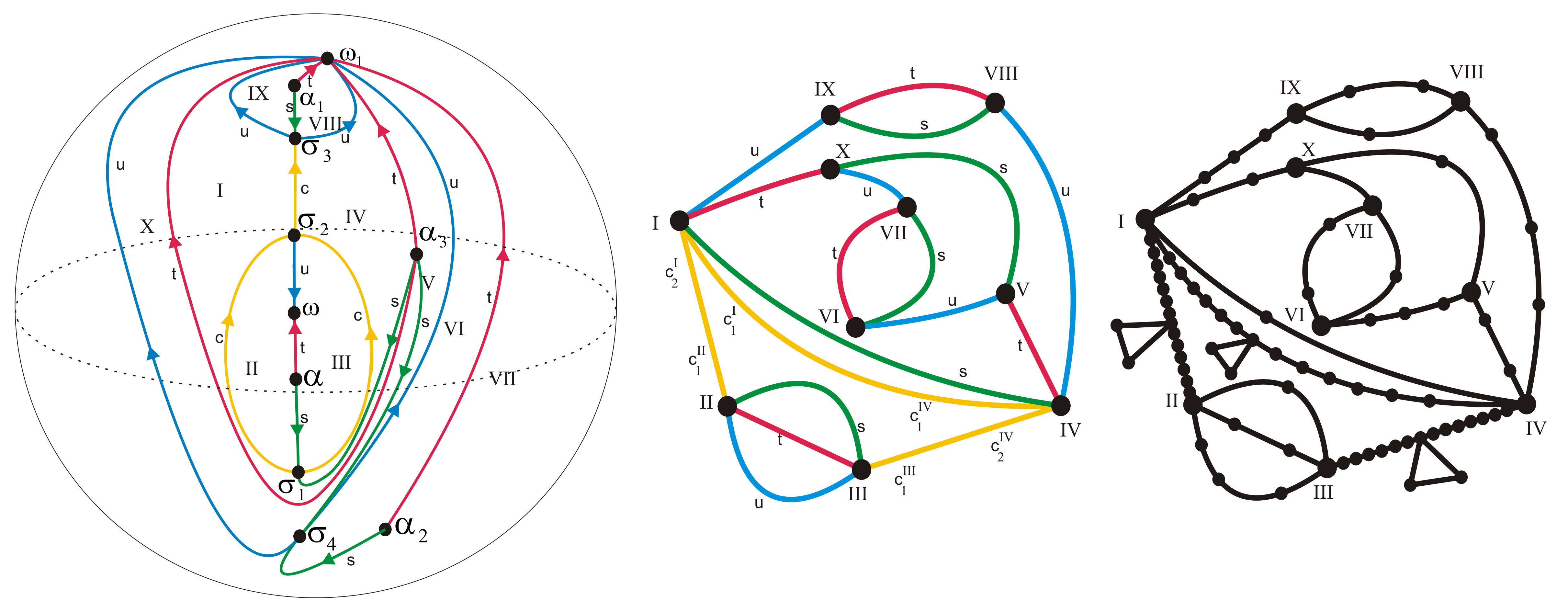 Figure 1
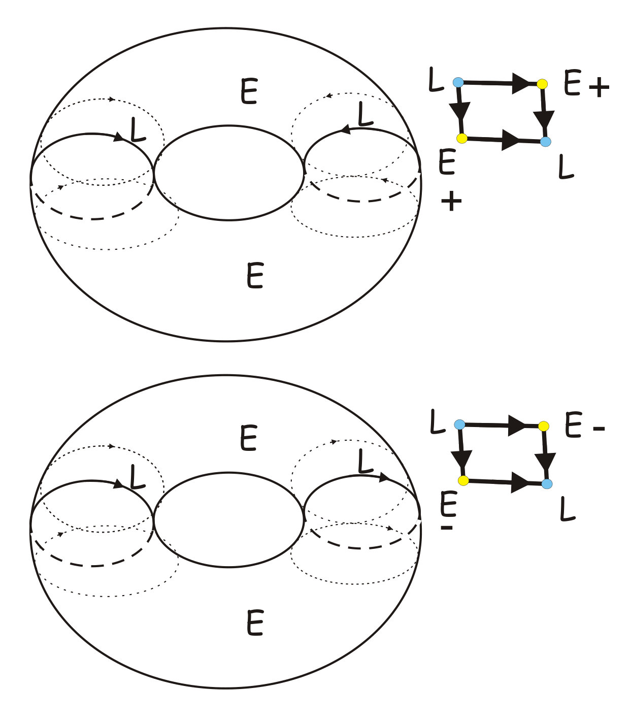 Figure 2
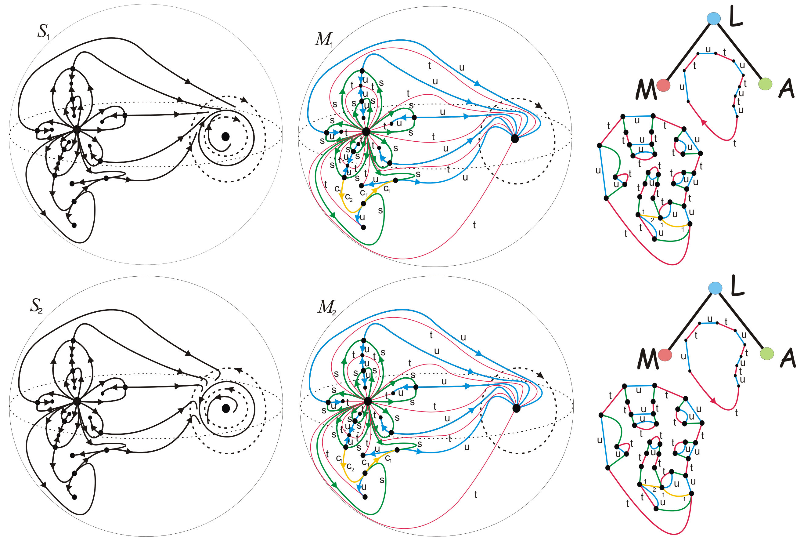 Figure 3
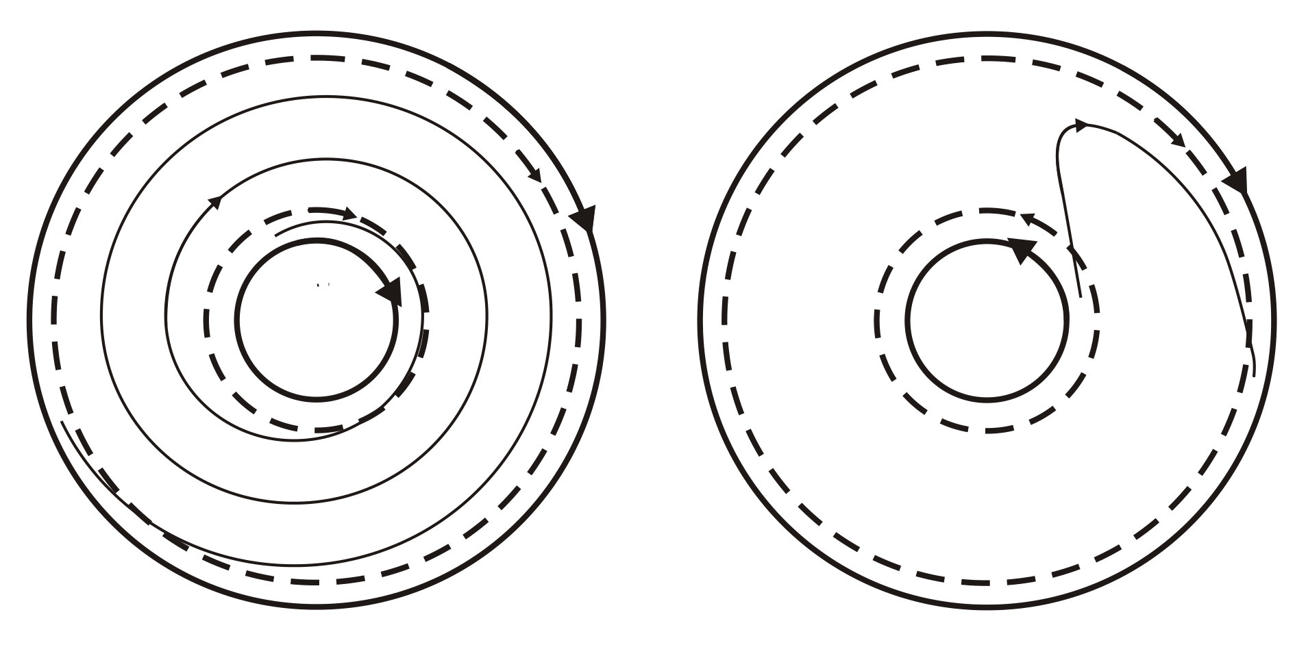 Figure 4
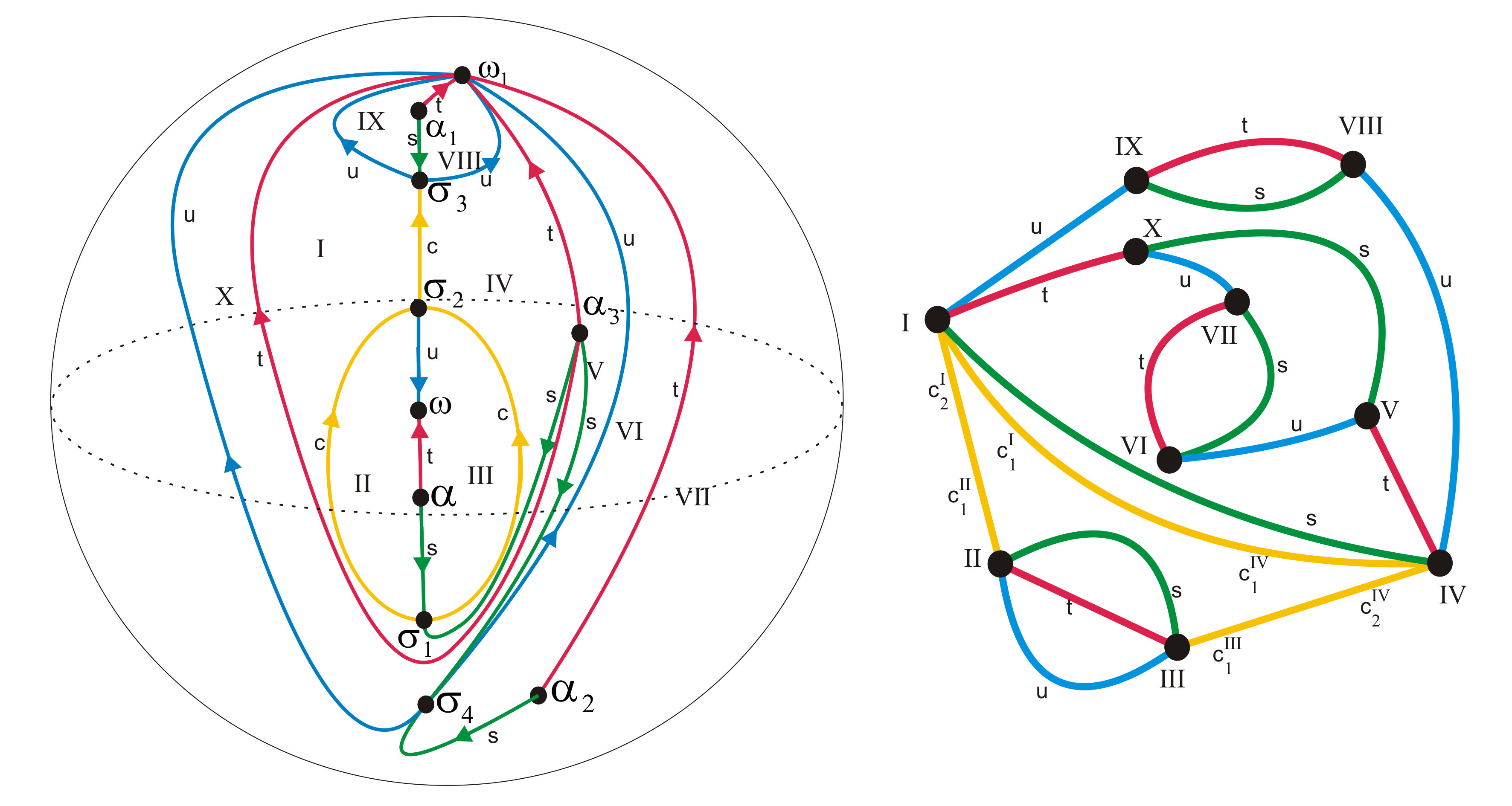 Figure 5
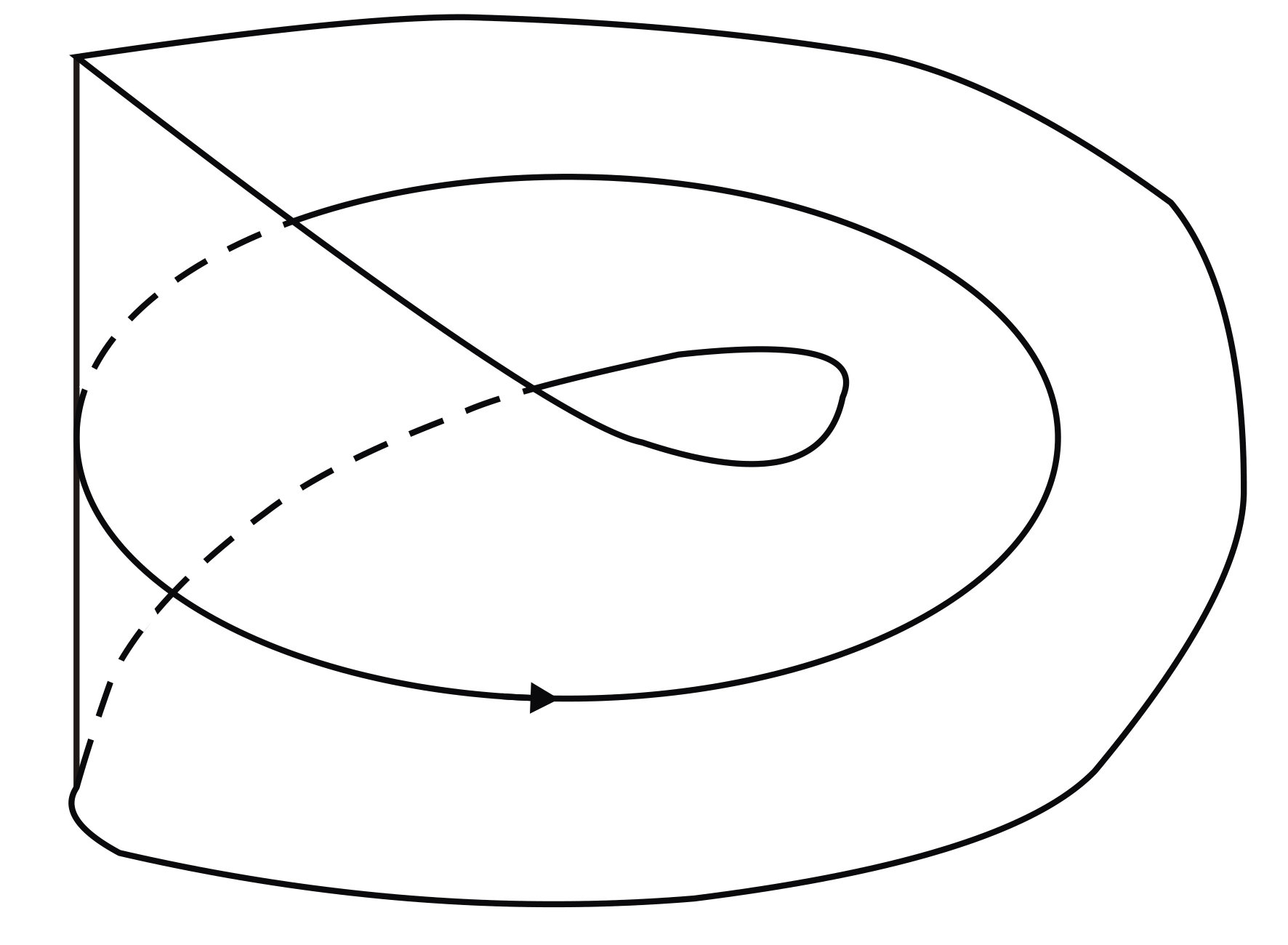 Figure 6
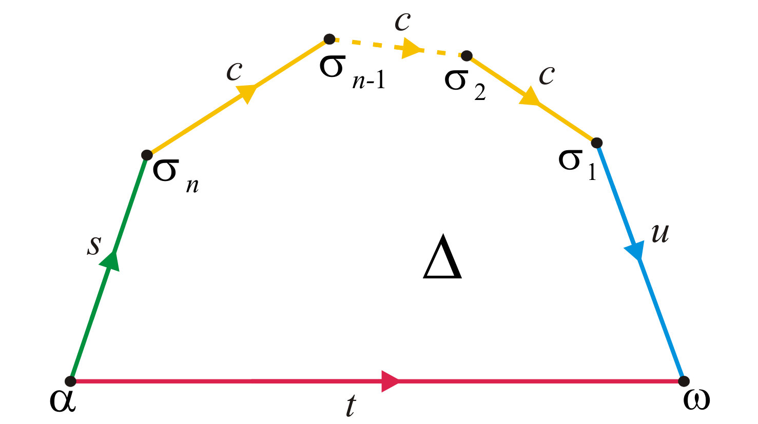 Figure 7
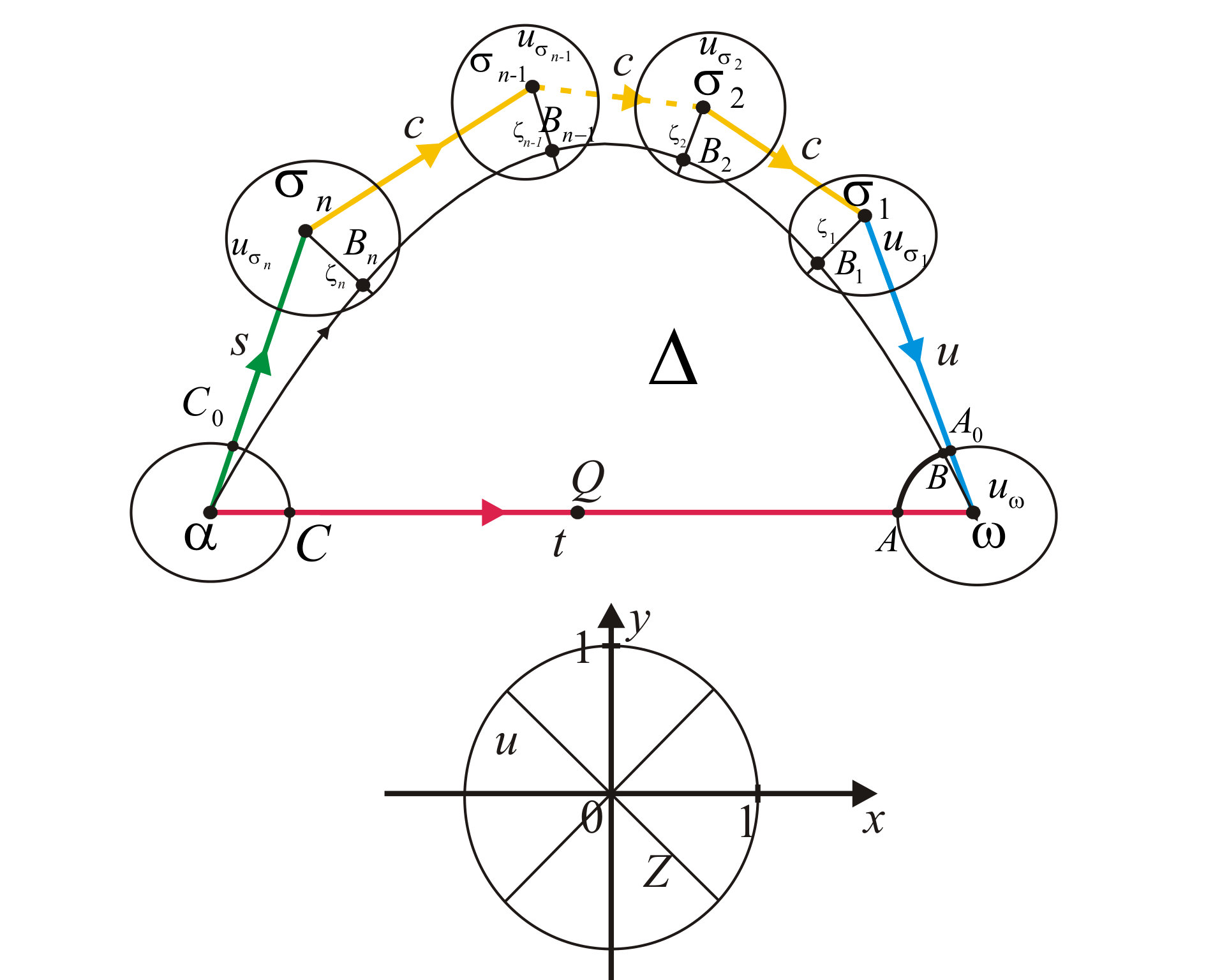 Figure 8
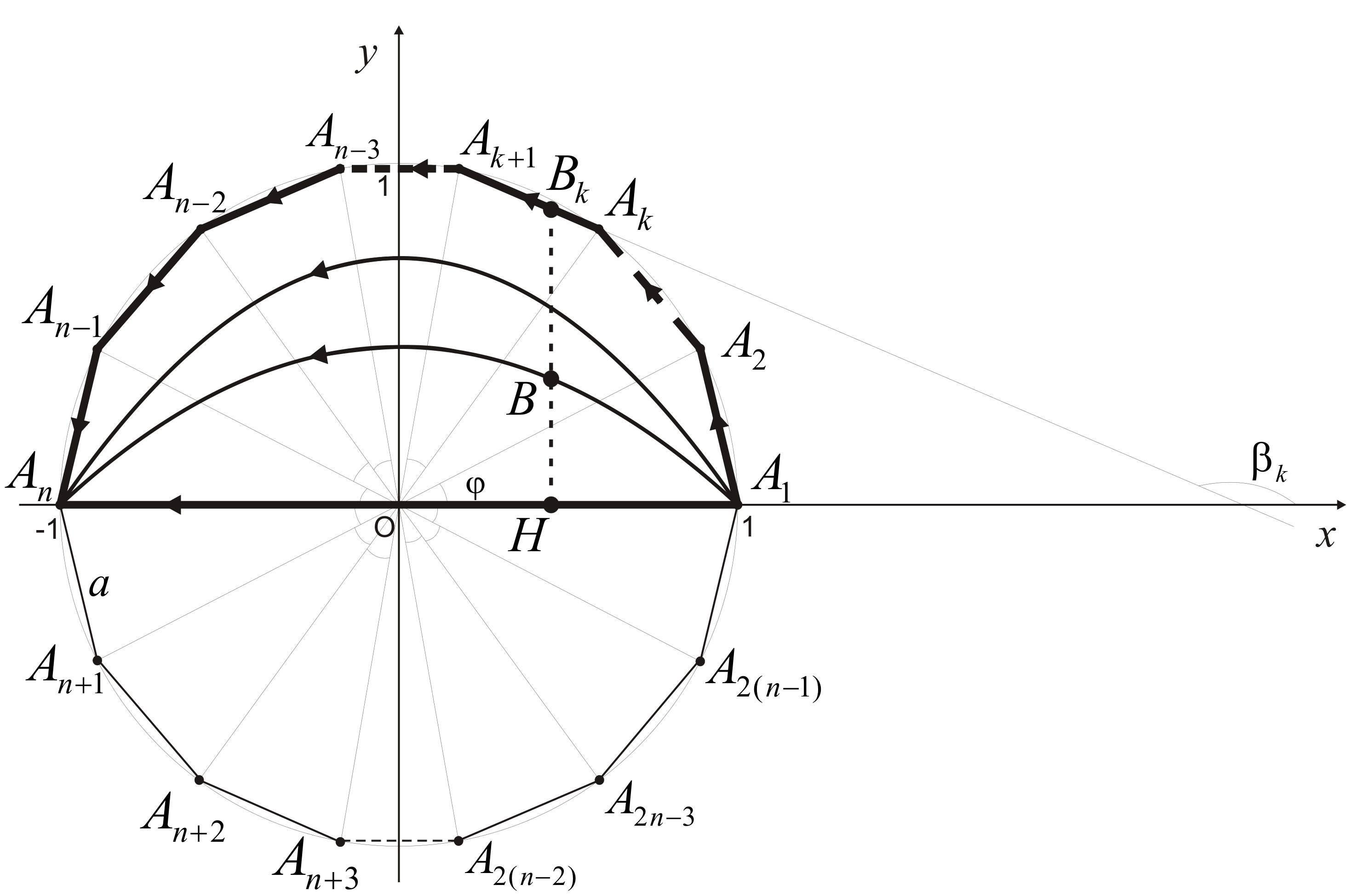 Figure 9
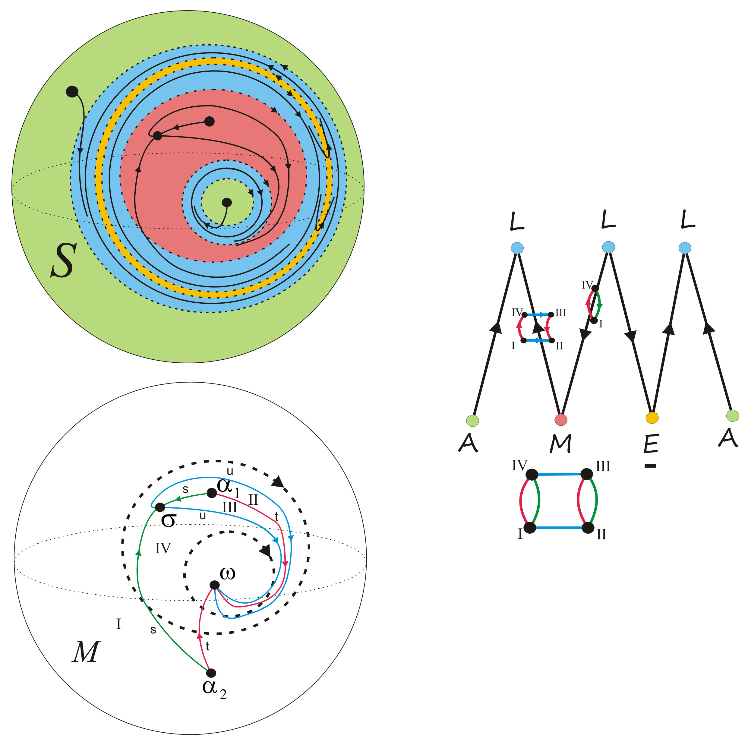 Figure 10
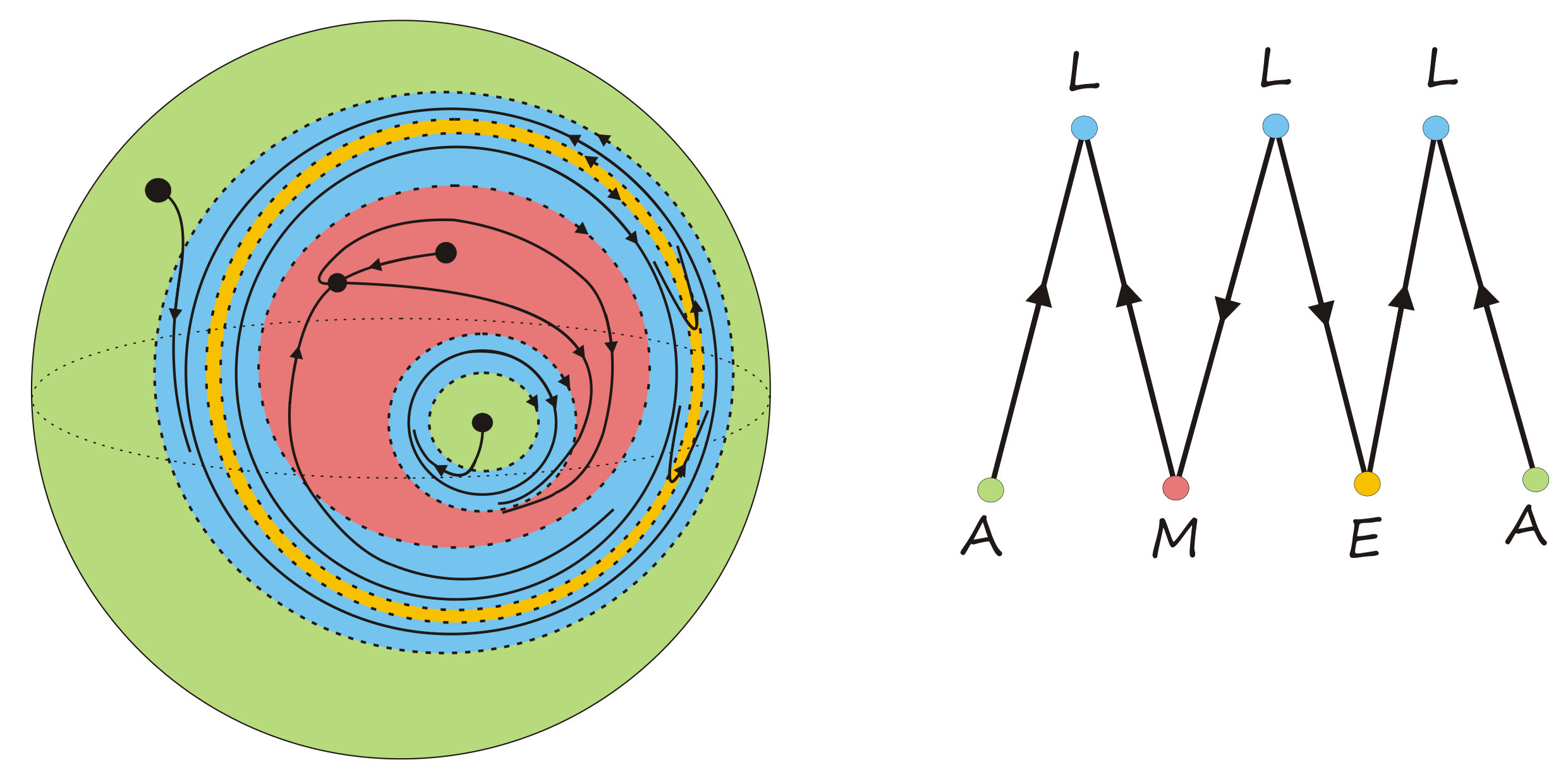 Figure 11
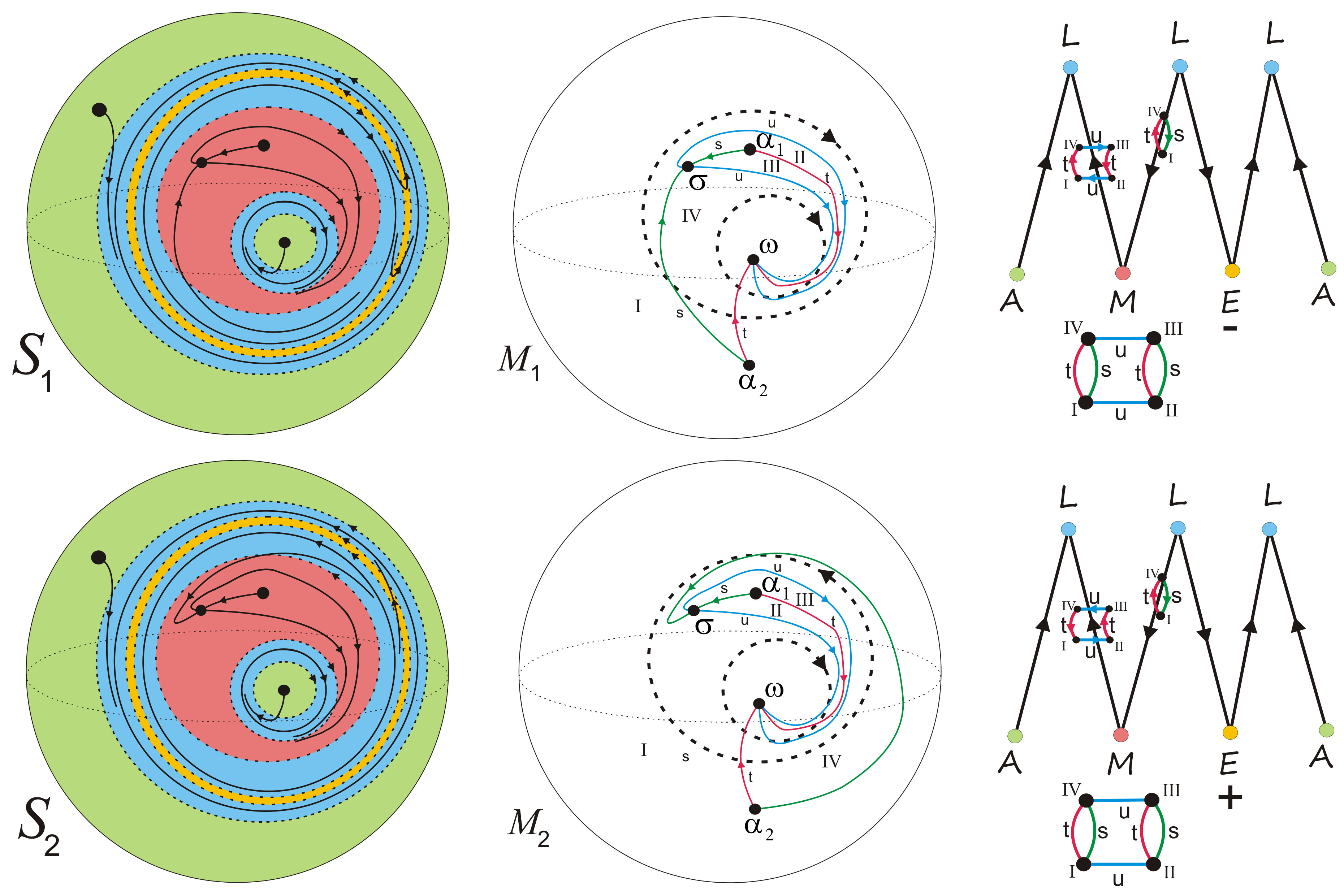 Figure 12
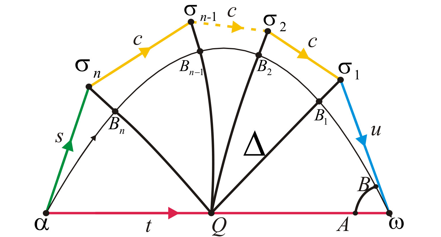 Figure 13
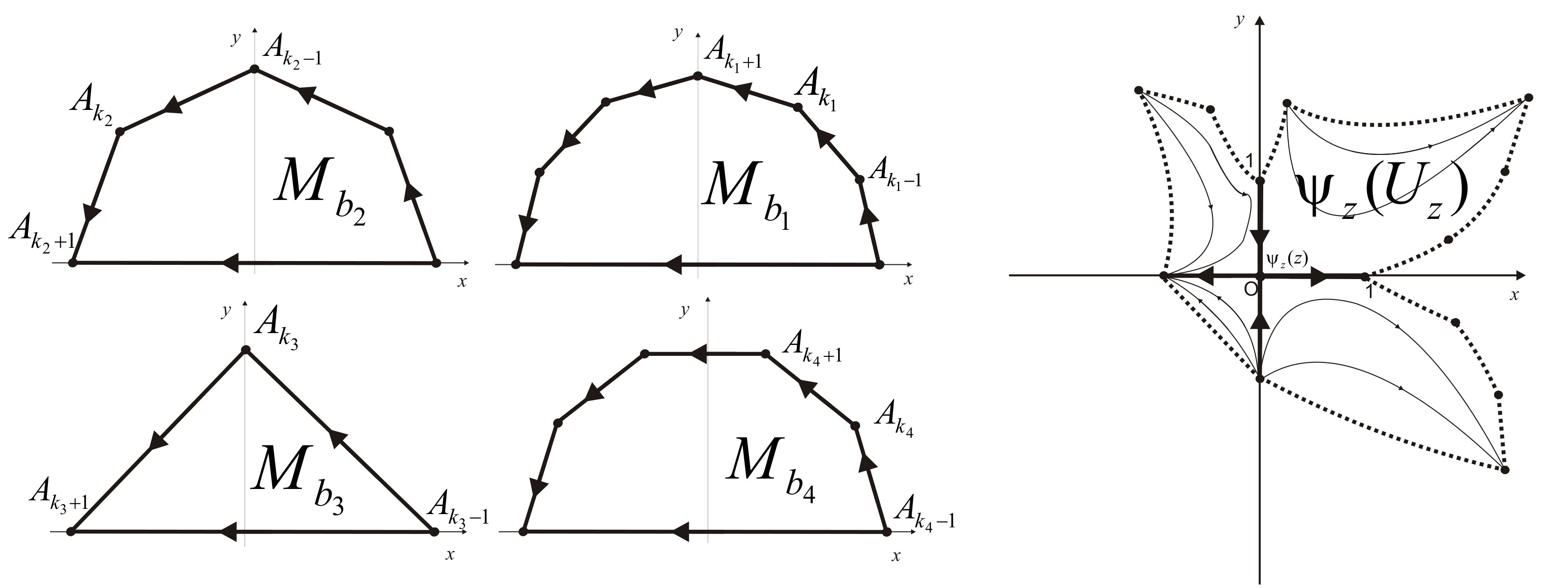 Figure 14
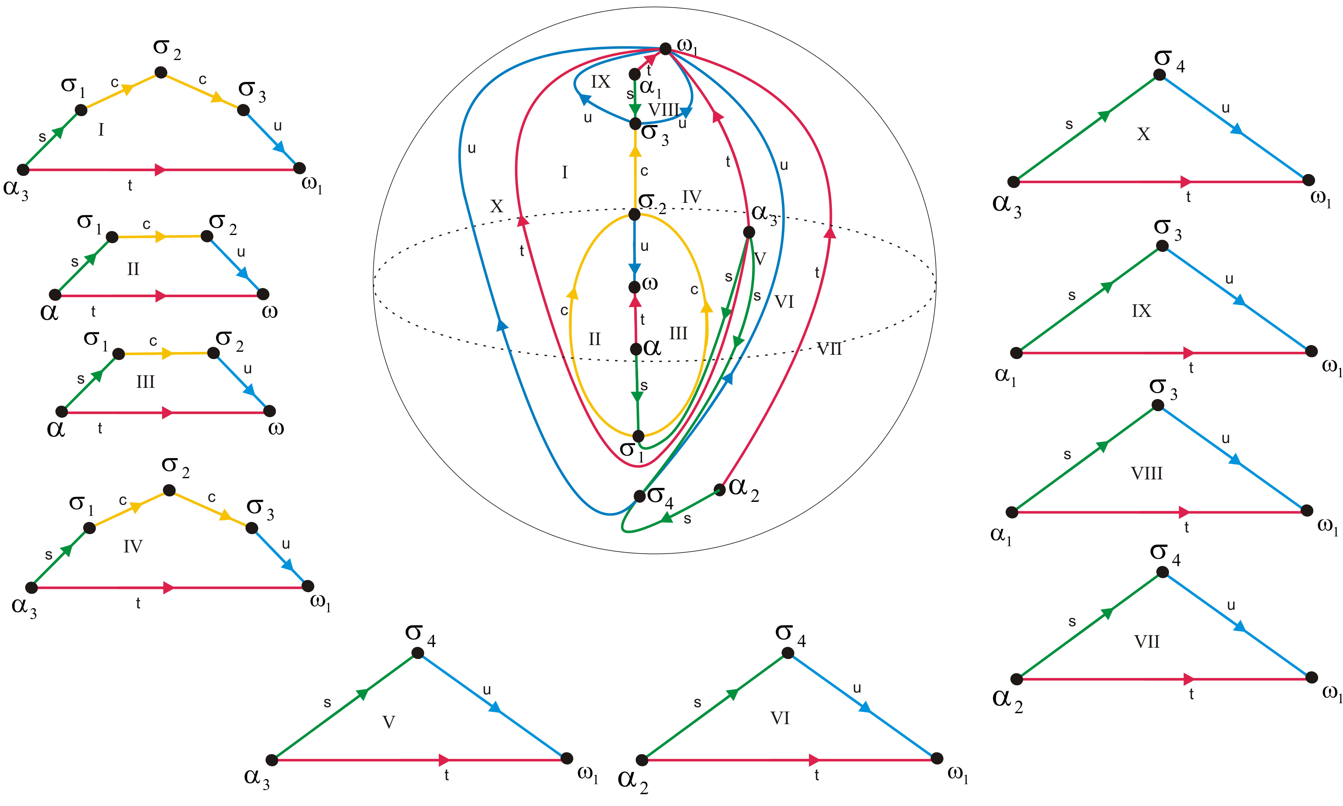 Figure 15
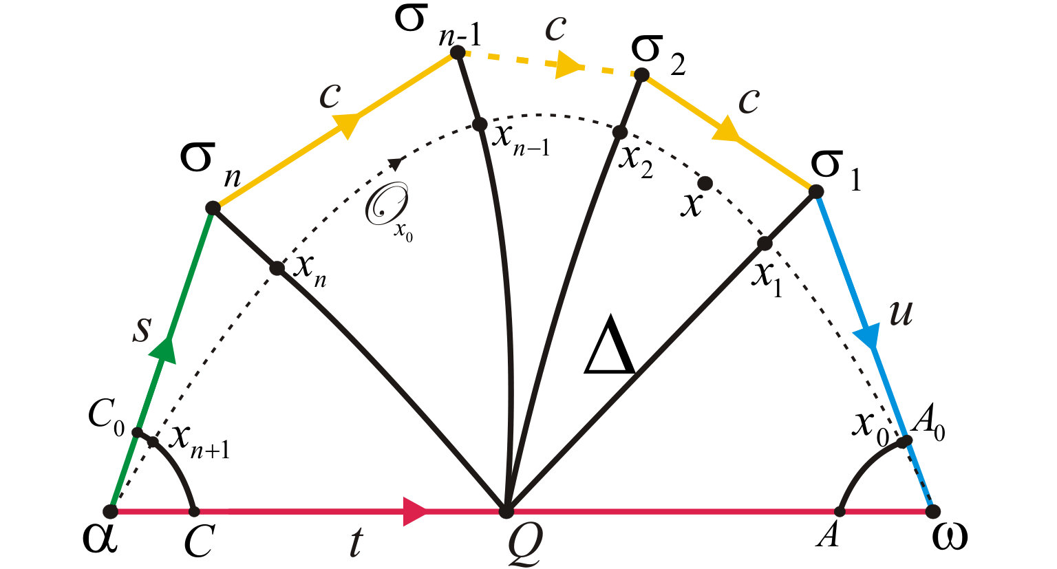 Figure 16
Peer Reviews
No public reviews on file for this paper yet. If you reviewed it on a platform where reviews are public (OpenReview, ICLR, NeurIPS, ICML), you can paste yours below so the community can read it here.
Videos
No videos yet. Explain this paper in a talk, walkthrough, or lecture? Add one.
Taxonomy
TopicsMathematical Dynamics and Fractals · Topological and Geometric Data Analysis
Vladislav E. Kruglov111HSE Campus in Nizhny Novgorod, Faculty of Informatics, Mathematics, and Computer Science, Laboratory of Topological Methods in Dynamics. Trainee Researcher. Lobachevsky State University of Nizhny Novgorod, Institute ITMM, Department of Mathematical Physics and Optimal Control. Master’s student; E-mail: [email protected], Dmitry S. Malyshev222HSE Campus in Nizhny Novgorod, Laboratory of Algorithms and Technologies for Networks Analysis. Leading Research Fellow. HSE Campus in Nizhny Novgorod, Faculty of Informatics, Mathematics, and Computer Science, Department of Applied Mathematics and Informatics. Professor. Lobachevsky State University of Nizhny Novgorod, Institute ITMM, Department of Algebra, Geometry and Discrete Mathematics. Professor; Doctor of Sciences; E-mail: [email protected], Olga V. Pochinka333HSE Campus in Nizhny Novgorod, Faculty of Informatics, Mathematics, and Computer Science, Department of Fundamental Mathematics. Professor, Department Head. HSE Campus in Nizhny Novgorod, Faculty of Informatics, Mathematics, and Computer Science, Laboratory for Topological Methods in Dynamics. Laboratory Head; Doctor of Sciences; E-mail: [email protected]
TOPOLOGICAL CLASSIFICATION OF -STABLE FLOWS ON SURFACES BY MEANS OF EFFECTIVELY DISTINGUISHABLE MULTIGRAPHS444The authors are grateful to the participants of the seminar “Topological methods in dynamics” for fruitful discussions. The classification and realisation results (Sections 1–8 without Subsection 5.3) were obtained with the support of the Basic Research Program at the HSE (project 90) in 2017. The algorithmic results (Subsection 5.3, Section 9) were obtained with the support of Russian Foundation for Basic Research 16-31-60008-mol-a-dk and RF President grant MK-4819.2016.1.
Structurally stable (rough) flows on surfaces have only finitely many singularities and finitely many closed orbits, all of which are hyperbolic, and they have no trajectories joining saddle points. The violation of the last property leads to -stable flows on surfaces, which are not structurally stable. However, in the present paper we prove that a topological classification of such flows is also reduced to a combinatorial problem. Our complete topological invariant is a multigraph, and we present a polynomial-time algorithm for the distinction of such graphs up to an isomorphism. We also present a graph criterion for orientability of the ambient manifold and a graph-associated formula for its Euler characteristic. Additionally, we give polynomial-time algorithms for checking the orientability and calculating the characteristic.
JEL Classification: C69; MSC Classification: 37D05.
Keywords: -stable flow, topological invariant, multigraph, four-colour graph, polynomial-time, algorithms.
1 Introduction
A traditional method of qualitative studying of a flows dynamics with a finite number of special trajectories on surfaces consists of a splitting the ambient manifold by regions with a predictable trajectories behavior known as cells. Such a view on continuous dynamical systems rises to the classical work by A. Andronov and L. Pontryagin [2] published in 1937. In that paper, they considered a system of differential equations
[TABLE]
where is a -vector field given on a disc bounded by a curve without a contact in the plane and found a roughness criterion for the system (1).
A more general class of flows on the 2-sphere was considered in works by E. Leontovich-Andronova and A. Mayer [13, 14], where a topological classification of such flows was also based on splitting by cells, whose types and relative positions (the Leontovich-Mayer scheme) completely define a qualitative decomposition of the phase space of the dynamical system into trajectories. The main difficulty in generalisations of this result to flows on arbitrary orientable surfaces is the possibility of new types of trajectories, namely unclosed recurrent trajectories. The absence of non-trivial recurrent trajectories for rough flows on the plane and on the sphere is an immediate corollary from the Poincaré-Bendixson theory for these surfaces, but this is not so trivial for orientable surfaces of genus . At first, it was proved by A. Mayer [15] in 1939 for rough flows with no singularities on the 2-torus555Actually in [15] A. Mayer found the conditions of roughness for cascades (discrete dynamical systems) on the circle and he also got the topological classification for these cascades. and later by M. Peixoto [20, 21] for structurally stable666The term “rough system” introduced by A. Andronov and L. Pontryagin in [2] is slightly different from its English counter part “structurally stable system” introduced by M. Peixoto in [20, 21], but the sets of rough and structural stable systems coincide. flows on surfaces of any genus (see also [19]).
In 1971, M. Peixoto obtained a topological classification of structurally stable flows on arbitrary surfaces [22]. As before, he did it by studying all admissible cells and he introduced a combinatorial invariant called a directed graph generalizing the Leontovich-Mayer scheme. In 1976, D. Neumann and T. O’Brien [17] considered the so-called regular flows on arbitrary surfaces, such flows have no non-trivial periodic trajectories (i.e. periodic trajectories other than limit cycles) and include the flows above as a particular case. They introduced a complete topological invariant for the regular flows named an orbit complex, which is a space of flow orbits equipped with some additional information.
In 1998, A. Oshemkov and V. Sharko [18] introduced a new invariant for Morse-Smale flows on surfaces, namely a three-colour graph, and described an algorithm to distinct such graphs, which was not, however, polynomial, i.e. its working time is not limited by some polynomial on the length of input information. In the same work they obtained a complete topological classification of Morse-Smale flows on surfaces in terms of atoms and molecules introduced in the work of A. Fomenko [3].
Structurally stable (rough) flows on surfaces have only finitely many singularities and finitely many closed orbits, all of which are hyperbolic, they also have no trajectories joining saddle points. The violation of the last property leads to -stable flows on surfaces, which are not structural stable. However, in the present paper we prove that a topological classification of such flows is also reduced to a combinatorial problem. The complete topological invariant is an equipped graph and we give a polynomial-time algorithm for the distinction of such graphs up to isomorphism. We also present a graph criterion for orientability of the ambient manifold and a graph-associated formula for its Euler characteristic. Additionally, we give polynomial-time algorithms for checking the orientability and calculating the characteristic.
2 The dynamics of an -stable flow
Let be some -stable flow on a closed surface . The non-wandering set of the flow consists of a finite number of hyperbolic fixed points and hyperbolic closed trajectories (limit cycles), which are called basic sets.
Denote by a class of -stable flows with at least one fixed saddle point or at least one limit cycle777If flow has neither fixed saddle points nor closed trajectories, then its non-wandering set consists of exactly two fixed points: a source and a sink, all such flows are topologically equivalent, that is the reason we exclude such flows from the class . on a surface . That is the flow class we consider in our work.
2.1 Fixed points
Let .
The hyperbolicity of the fixed points is expressed by the following fact.
Proposition 2.1** ([19], Theorem 5.1 from Chapter 2 and [24], Theorem 7.1 from Chapter 4).**
The flow in some neighbourhood of a fixed point is topologically equivalent to one of the following linear flows
[TABLE]
In the cases , , the fixed point is called sink, saddle, source and has the dimension of the unstable manifold equal to accordingly. We will denote by , , the set of all sinks, saddles, sources of accordingly.
It follows from the criterion of the -stability in [23] that the saddle points do not organize cycles, i.e. collections of points
[TABLE]
with a property
[TABLE]
2.2 Closed trajectories
Let be a closed trajectory of and . Let be a smooth cross-section passing through the point transversal to trajectories of near . Let be a neighbourhood of such that for every point the value with properties and for any is well-defined. Then is called a Poincaré’s cross-section and a map given by the formula is called Poincaré’s map.
The hyperbolicity of the closed trajectory is expressed by the following fact.
Proposition 2.2** ([19], Proposition 1.2 from Chapter 3 and Theorem 5.5 from Chapter 2).**
Poincaré’s map is a diffeomorphism with a fixed point in a neighbourhood of which is topologically conjugate to one of the following linear diffeomorphisms
[TABLE]
In the cases the closed trajectory is called attractive, repelling limit cycle accordingly. Denote by the set of all limit cycles of .
In any case the limit cycle has a neighbourhood , avoiding other limit cycles and fixed points of and with the transversal to the trajectories of boundary . The neighbourhood is homeomorphic to the annulus or the Möbius band (see Fig. 1) in the cases or accordingly and can be constructed the following way.
For every points let us denote by the segment of bounded by the points and by the length of this segment. In the cases let us choose points on different connected components of . Then is a union of two circles
[TABLE]
In the cases let us choose a point . Then
[TABLE]
A moving of along the trajectories in the positive time gives a consistent with orientation on . Thus, in further we will assume that is oriented consistently with .
3 The directed graph for a flow
Recall that a graph is an ordered pair such that is a finite non-empty set of vertices, is a set of pairs of the vertices called edges. Besides, if is a multiset then is called multigraph. Recall that a multiset is a set with the opportunity of multiple inclusion of its elements. Everywhere below we will call a multigraph simply as a graph.
If a graph includes an edge , then both vertices and are called incident to the edge . The vertices and are connected by . A graph is called directed if every its edge is an ordered pair of vertices. A finite sequence
[TABLE]
of vertices and edges of a graph is called a path, the number is called the length of the path and it is equal to the number of edges of the path. The path is called simple if it contains only pairwise disjoint edges. The simple path is called a cycle if . A graph is called connected if every two its vertices can be connected by a path.
Let . We call a cutting set and the connected components of cutting circles. Let . We call an elementary region a connected component of the set . The elementary regions, obviously, can be of the following pairwise disjoint types with respect to information about basic sets of in the regions:
-
a region of the type contains exactly one limit cycle;
-
a region of the type contains exactly one source or exactly one sink;
-
a region of the type contains at least one saddle point;
-
a region of the type does not contain elements of basic sets.
Definition 1**.**
A directed graph is said to be a graph of the flow (see Fig. 2) if
(1) the vertices of bijectively correspond to the elementary regions of ;
(2) every directed edge of , which joins a vertex with a vertex , corresponds to the cutting circle , which is a common boundary of the regions and corresponding to and , such that any trajectory of passing goes from to by increasing the time.
We will call a -, -, - or -vertex a vertex of , which corresponds to a -, -, - or -region accordingly.
The following proposition immediately follows from the dynamics of the flow and a structure of cutting set.
Proposition 3.1**.**
Let be the directed graph of a flow , then:
1) every -vertex can be connected only with -vertices, furthermore, with every vertex by a single edge;
2) every -vertex can be incident only to two edges that connect this vertex with two different -vertices, and one of these edges enters to the -vertex, another one exits;
3) every -vertex can be connected only with a -vertex, furthermore, by a single edge;
4) every -vertex has degree (the number of incident edges) 1 or 2, and if its degree is 2, then both edges either enter the vertex or exit.
The existence of an isomorphism of the directed graphs for topologically equivalent -stable flows from is a necessary condition. To make the directed graph a complete topological invariant for the class , below we equip the graph by additional information.
4 Equipment of the directed graph
In this section, we describe how to assign some additional information to vertices and edges of the directed graph of a flow from .
4.1 -vertex
The flows in -regions can belong to only the two equivalence classes: a source pool and a sink pool, which we can distinguish by directions of edges incident to -vertices.
4.2 -vertex
The flows in -regions can belong to only the four equivalence classes: an annulus with a stable limit cycle, an annulus with an unstable one, the Möbius band with a stable one, the Möbius band with an unstable one, which we can distinguish by directions of edges and by quantities of edges incident to -vertices.
4.3 -vertex
The flows in -regions can belong to only the two equivalence classes corresponding to the consistent and the inconsistent orientation of connecting components of ’s boundary. However, a structure of an -region cannot be determined by the directed graph, therefore, we will attribute the weight to the vertex corresponding to an -region. The weight is ‘‘’’ in the consistent case and ‘‘’’ in the inconsistent one.
4.4 -vertex
The flows in -regions cannot be determined by the directed graph. Then we will equip vertices corresponding to them by four-colour graphs for a description of the dynamics of the flow in the regions. In more details.
All results about flows from without periodic trajectories are given and proved in our paper [11] but we give it here for completness.
Let us consider some -region that is either a 2-manifold with a boundary or a closed surface. In the first case let us attach the union of disjoint 2-disks to the boundary to get a closed surface , in the second case we also denote the closed surface by and will suppose that . Let us extend up to an -stable flow assuming that coincides with out of and has exactly one fixed point (a sink or a source) in each connected component of .
Let be the sets of all sources, saddle points and sinks of accordingly. By the definition of the region the flow has at least one saddle point. Let
[TABLE]
A connected component of is called a cell.
Lemma 4.1**.**
Every cell of the flow contains a single sink and a single source in its boundary, and the whole cell is the union of trajectories going from to .
Let us choose a trajectory in the cell , we will call it a -curve. Let
[TABLE]
Let us call a -curve a separatrix connecting saddle points (from the word ‘‘connection’’), a -curve an unstable saddle separatrix with a sink in its closure, a -curve a stable saddle separatrix with a source in its closure. We will call a polygonal region the connecting component of .
Lemma 4.2**.**
Every polygonal region is homeomorphic to an open disk and its boundary consists of an unique -curve, an unique -curve, an unique -curve, and a finite (may be empty) set of -curves (see Fig. 4).
Denote by the set of all polygonal regions of (see Fig. 5, where a flow and all its polygonal regions are presented).
Definition 2**.**
A multigraph is called -colour graph if the set of its edges is the disjoint union of subsets, each of which consists of edges of the same colour.
We say that a four-colour graph with edges of colours bijectively corresponds to if:
-
the vertices of bijectively correspond to the polygonal regions of ;
-
two vertices of are incident to an edge of colour , , or if the polygonal regions corresponding to these vertices has a common -, -, - or -curve; that establishes an one-to-one correspondence between the edges of and the colour curves;
-
if some vertex of is incident to more than one -edge (the number of -edges is more than ), then -edges are ordered
[TABLE]
by a moving (according to the direction from the source to the sink on -curve) along the boundary of the corresponding polygonal region (see, for example, Figure 6).
Definition 3**.**
We say that the graph is the four-colour graph of the flow corresponding to .
Definition 4**.**
Two four-colour graphs and corresponding to and respectively are said to be isomorphic if there is an one-to-one correspondence of vertices and edges of the first graph to vertices and edges of the second graph preserving colours of all edges and numbers of -edges.
4.5 - and -edge
Let us denote by the one-to-one correspondence described above between polygonal regions and vertices, also between colour curves of and colour edges of respectively.
Let us call a -cycle (-cycle) a cycle of consisting only of - and -edges (- and -edges). Let us call - and -edges exiting out a vertex as nominal -edges and assign the numbers [math] and to them respectively. Let us call a -cycle a simple cycle
[TABLE]
if
[TABLE]
Proposition 4.1**.**
The projection gives an one-to-one correspondence between the sets , , and the sets of -, -, and -cycles respectively.
By our construction , where is either empty or each its connected component contains exactly one sink (source ) of the flow , uniquely corresponding to a cutting circle for a limit cycle of the flow , which uniquely corresponds to a -edge (-edge) of the graph . Due to Proposition 4.1 the node () uniquely corresponds to a -cycle (a -cycle), denote it by (). Moreover, due to Proposition 4.1, we can embed the graph such that the cycle () coincides with . Thus we induce an orientation from to the cycle and call the cycle () oriented one.
5 The formulation of the results
Definition 5**.**
Let be the directed graph of a flow . We will say that is the equipped graph of and denote it by if:
(1) every -vertex is equipped with the weight ‘‘’’ or ‘‘’’ in consistent and inconsistent case respectively;
(2) every -vertex is equipped with a four-colour graph corresponding to the flow constructed in Subsection 4.4;
(3) every edge () is equipped with an oriented -cycle (-cycle) () of corresponding to the limit cycle of and oriented consistently with (see Fig. 7).
On Fig. 8 you can see the two examples of flows from whose difference might be defined only by oriented cycles equipping their graphs, and on Fig. 9 – by weight of -vertices.
Let us denote by the one-to-one correspondence described above between the elementary regions and the vertices, the cutting circles and the edges, the directions of the trajectories and the directions of the edges, the consistencies of the orientations of the boundary’s connecting components of -regions and the weights of the -vertices, the -regions and the four-colour graphs, the stable limit cycles and the -cycles, the unstable limit cycles and the -cycles, the orientations of the stable limit cycles and the orientations of the cycles , the orientations of the unstable limit cycles and the orientations of the cycles accordingly.
5.1 The classification result
Definition 6**.**
Equipped graphs and are said to be isomorphic if there is an one-to one correspondence between all edges and vertices of and all edges and vertices of preserving their equipments in the following way:
(1) the weights of vertices and are equal;
(2) for vertices and , there is an isomorphism of the four-colour graphs such that and the orientations of and coincide (similarly for ).
Theorem 1**.**
Flows are topologically equivalent if and only if the equipped graphs and are isomorphic.
5.2 The realisation results
To solve the realization problem, we introduce the notion of an admissible four-colour graph and an equipped graph.
Let be a four-colour graph with the properties:
(1) every edge of the four-colour graph is coloured in one of the four colors: ;
(2) every vertex of the four-colour graph is incident to exactly one edge of the colours . Besides, the number of -edges incident to a vertex can be any (may be null) and these edges are ordered if .
Definition 7**.**
The graph we call an admissible four-colour graph if it contains -cycles and every such a cycle has four vertices.
Lemma 5.1**.**
The graph is admissible.
Lemma 5.2**.**
Every admissible four-colour graph corresponds to a closed surface and an -stable flow from without limit cycles, besides:
(1) The Euler characteristic of can be calculated by the formula
[TABLE]
where are the numbers of all -, - and -cycles of respectively;
(2) is non-orientable if and only if has at least one cycle with an odd length.
Definition 8**.**
We call an admissible equipped graph if it is a connected directed graph with -, -, - and -vertices satisfying the items (1)–(4) of Proposition 3.1, so that
– every -vertex is equipped with an admissible four-colour graph ,
– every edge entering to (exiting out of) any -vertex is equipped with an oriented -cycle (-cycle) of the four-colour graph,
– every -vertex is assigned with a weight ‘‘’’ or ‘‘’’.
Lemma 5.3**.**
The graph is admissible.
For every -vertex of an admissible equipped graph , let us denote by the result of applying the formula (2) to the corresponding admissible four-colour graph . Denote by the quantity of edges, which are incident to and denote by the quantity of -vertices of .
Theorem 2**.**
Every admissible equipped graph corresponds to an -stable flow from on a closed surface , besides:
(1) The Euler characteristic of can be calculated by the formula
[TABLE]
(2) is orientable if and only if every four-colour graph equipping has not cycles of an odd length and every -vertex is incident to exactly two edges.
5.3 The algorithmic results
An algorithm for solving the isomorphism problem is considered to be efficient if its working time is bounded by a polynomial on the length of the input data. Algorithms of such kind are also called polynomial-time or simply polynomial. This commonly recognized definition of efficient solvability rises to A. Cobham [5]. A common standard of intractability is NP-completeness [6]. The complexity status of the isomorphism problem is still unknown, i.e., for the class of all graphs, neither its polynomial-time solvability nor its NP-completeness is proved at the moment. Fortunately, four-colour graphs and directed graphs of flows are not graphs of the general type, as they can be embedded into a fixed surface on which flows are defined, i.e. the ambient surface. That allows to prove the following theorems.
Theorem 3**.**
Isomorphism of the equipped graphs , of flows , can be recognized in polynomial time.
Theorem 4**.**
The orientability of the ambient surface for an -stable flow can be tested in a linear time and the Euler characteristic of can be determined in quadratic time by means of the equipped graph .
6 The dynamics of a flow without limit cycles on a surface
In this section everywhere below is a flow without limit cycles on a closed surface . We give proofs for the results from Subsection 4.4 and other results about flows without limit cycles. A part of them was proved in [12], [11] and [7] but we repeat them for a completeness.
6.1 General properties
Firstly let us give a necessary proposition, which we will use for the proof of the classification theorem.
Proposition 6.1** ([7], Theorem 2.1.1).**
**
1) ;
2) is a smooth submanifold of diffeomorphic to for every fixed point .
Let be a fixed point of . Let us denote by () the unstable (stable) separatrix of .
Lemma 6.1**.**
For every sink (source ) of there is at least one saddle point with an unstable separatrix (a stable separatrix ) such that .
Proof.
Supposing the contrary for some sink , we get by the item 1) of Proposition 6.1 that , where is a source such that . Let us show that .
Let us assume the contrary. Then, by the item 1) of Proposition 6.1, there is a point such that and . Let and be points such that and . As the manifold is homeomorphic to by the item 2) of Proposition 6.1, then there is a simple path connecting with . Then, there is a value such that and for . Consequently, there is a point such that and . Besides, the point . But if , then for some and, consequently, that is the contradiction with the definition of the unstable manifold of a fixed point.
We have got that for any and, hence, the set is open as it contains every point with some open neighbourhood. As is both open and closed, . Then does not contain saddle points, that contradicts with conditions of the lemma.
The affirmation for sources can be proved by conversion from to . ∎
Lemma 6.2**.**
Let be a fixed point of . Then
* if , then*
[TABLE]
* if , then , where is a non-empty subset of .*
Proof.
Consider the case , where is a saddle point. Let . Any point of is a point of for some fixed point by the item 1) of Proposition 6.1. The point can be: a) a sink; b) a saddle point; c) a source.
a) Let us consider a sink such that . As is the source and , where is the orbit of , then . So .
b) Let us consider a saddle point such that . In this case . So .
c) Assume that there is a source such that . As , then , which is impossible because consists of wandering points. Consequently, the case c) is impossible.
Consider the case : is a source.
The item 1) of Proposition 6.1 says that the set is -invariant subset of . Then, for the proof of our Lemma all we need is to prove that a) if for some , then and b) if for some , then there is such that and .
a) As , there is a sequence such that for . Then and, due to the known behaviour of our flow near (see, Proposition 2.1), the set contains in its closure the separatrix .
b) Let . According to Lemma 6.1 there is a finite set of saddle points such that for . Then the set consists of a finite number of connected components, at least one of them belongs to , denote it by . Thus there is at least one saddle point whose separatrices belongs to . Thus . ∎
The statement similar to Lemma 6.2 may be proved for the stable separatrices of the flow .
6.2 The proof for Lemma 4.1
We remind that a cell is a connected component of the set .
Due to Proposition 6.1
[TABLE]
Then every connected component of is a subset of for a source . Similarly
[TABLE]
Then every connected component of is a subset of for a sink . Thus
[TABLE]
and, consequently, the cell is a union of trajectories going from to .
6.3 The proof for Lemma 4.2
We remind that we choose a one trajectory in the cell and called it by a -curve. Also we defined . Besides, we called by a -curve a separatrix connecting saddle points (‘‘connection’’), by a -curve an unstable saddle separatrix with a sink in its closure, by a -curve a stable saddle separatrix with a source in its closure. A polygonal region is the closure of a connecting component of .
Due to Lemma 4.1 every cell belongs to the basin of the source and, due to Lemma 6.2, is situated in between too (may be coincident) -curves. A polygonal region can be created by removal a -curve from . As is homeomorphic to , due to Proposiition 6.1, then is homeomorphic to a sector in , i.e. is homeomorphic to an open disk. By construction, the boundary of contains unique -curve and unique -curve. As belongs to the basin of the sink in the same time, then it is restricted by unique -curve. By of Lemma 6.2 the region is restricted by a finite number of -curves. We have got that the only possible structure of the boundary of a polygonal region is the structure depicted on Figure 4 up to a number of the -curves.
6.4 The proof of Lemma 5.1
We remind that is the one-to-one correspondence between polygonal regions and vertices, also between colour curves of and colour edges of respectively.
As given on the surface and every vertex of corresponds to some its polygonal region, then, we can create a graph isomorphic to with each vertex in its own polygonal region and with edges that are curves embedded in , joining the vertices and crossing each its side at the unique point. Such graph is obviously isomorphic to . Therefore, without loss of generality, let’s mean that is embedded in . As every polygonal region side adjoins to exactly two different polygonal regions, then has not cycles of length , i.e. is simple one.
As to each point a finite number of polygonal regions divided by colour curves adjoins, then the point by means one-to-one corresponds to a cycle of the vertices corresponding to the regions adjoining to and of the colour edges crossing colour curves exiting out of . So exactly polygonal regions divided by -, - or -curves adjoin to a saddle point. If to mean - and -edges as nominal -edges, we get that every saddle point corresponds to the -cycle of . Conversely also is correct, because every -cycle can be placed in a neighbourhood of the single saddle point so that such neighbourhoods of different -cycles doesn’t cross one another. In this way contains -cycles and each such cycle has length . Consequently is admissible.
6.5 The proof of Proposition 4.1
The correspondence between and the set of -cycles follows from the proof of Lemma 5.1. The basin of every sink is divided by - and -curves alternately lying in . Consequently corresponds to unique -cycle of by means . Conversely it is also corrected because as basins of different sinks are divided by and -curves then each -cycle can be situated in the basin of the unique sink. In this way creates one-to-one corresponding between the set and the set of -cycles. The correspondence between and the set of -cycles can be proved similarly.
7 The proof for the classification Theorem 1
In this section we consider -stable flow on closed surface and prove that the isomorphic class of its equipped graph is a complete topological invariant.
7.1 The necessary condition of Theorem 1
Let two -stable flows given on a closed surface be topological equivalent, i.e. there is a homeomorphism mapping trajectories of to trajectories of . Let us think without loss of generality that the cutting set of is created so that , where is the cutting set of . Also we can think that the restriction of the set of -curves of to the -regions of is created so that , where is the restriction of the set of -curves of to the -regions of . Then maps the elementary and the polygonal regions of to the elementary and the polygonal regions of respectively.
Recall that is the one-to-one correspondence between the elementary regions and the vertices, the cutting circles and the edges, the directions of the trajectories and the directions of the edges, the consistencies of the orientations of the limit circles for the -regions and the weights of the -vertices, the -regions and the four-colour graphs, the stable limit cycles and the -cycles, the unstable limit cycles and the -cycles respectively. Let us define the isomorphism by the formula
[TABLE]
As carries out the topological equivalence of and then it preserves the types of elementary regions and, hence, preserves the types of the vertices. As preserves the orientation on the trajectories then the weights of vertices and are equal.
Let is the four-colour graph for some vertex , is the four-colour graph for the vertex . Recall that , and , is the one-to-one correspondence between the polygonal regions and the vertices, also between the colour curves of , and the colour edges of the four-colour graph , respectively.
As is the four-colour graph of the region , then . Let . As maps the polygonal regions of to the polygonal regions of , then there exists the isomorphism defined by the formula
[TABLE]
As , then and the orientations of and coincide (similarly for ). Thus is the required isomorphism.
7.2 The sufficient condition of Theorem 1
Let graphs and be isomorphic by means of . To prove the topological equivalence of the flows we need to create homeomorphisms between elementary regions mapping the trajectories of to the trajectories of so that for two elementary regions the homeomorphisms on their common boundaries coincide.
I. -region. Let us consider some -region of the flow . Consider the region
[TABLE]
of the flow . Their four-colour graphs and are isomorphic by means of . Let () be the flow corresponding to (). Recall that in Subsection 4.4 we defined the flow () on surface () such that () and ().
Consider a polygonal region . The ’s boundary contains an unique source , an unique sink and saddle points , and the saddle points are ordered so that their labels increase while moving along the ’s boundary according to the direction from the source to the sink on the -curve. Consider the polygonal region such that
[TABLE]
The isomorphism provides an equal number of the same-colour edges exiting out of graph vertices corresponding to and . It implies that ’s boundary contains exactly an unique source , an unique sink and saddle points ordered so that their labels increase while moving along the ’s boundary according to the direction from the source to the sink on the -curve. As preserves the colours of the edges and the numbers of the -edges, then for creation of the homeomorphism doing the topological equivalence of and all we need is to construct the homeomorphism mapping the trajectories of from to the trajectories of from so that
[TABLE]
for any polygonal regions , of .
Step 1. Let us construct in neighbourhoods of the node points. Let
[TABLE]
and recall that , are the flows given by the formulas , with the origin as a sink and a source point accordingly. By Proposition 2.1 there exist the neighbourhoods , (, ) of , (, ) accordingly such that , (, ) are topologically conjugate to , by means of some homeomorphisms , (, ) accordingly. Without loss of generality let us think that these neighbourhoods do not cross each other for all polygonal regions.
For let and , (, ). Let , (, ) and , (, ).
Everywhere below we will denote by the closure of a segment of a cross-section to the trajectories of () bounded by points () and (). In particular denote by () the segment which is the intersection () (see Figure 10). Let . Let () be the arbitrary homeomorphism such that (). Let
[TABLE]
Let () and () be the trajectory of (). Let , then for some and . Let us define the homeomorphism so that and , where . Similarly for points being the intersection point for some and , define the homeomorphism so that and , where .
Step 2. Let us construct on the boundary of .
Everywhere below we will denote by the closure of a segment of a trajectory or an separatrix of a saddle point bounded by points and , and by we will denote its length. Notice that and . For smooth segments , of trajectories of , we will call a homeomorphism by the length of arc a homeomorphism defined by the following rule for a point :
[TABLE]
Thus, we construct the following homeomorphisms: , , and .
A similar construction on the boundaries of all polygonal regions will provided for any polygonal regions , of .
Step 3. Let us construct cross-sections connecting the saddle points with some point inside ().
Let and . Let us construct cross-sections () the following way.
Recall that for there exists a neighbourhood () of () such that () is topologically conjugate to by means of some homeomorphism (), where and . Let
[TABLE]
The set consists of the two intervals crossing in the origin and transversal to the trajectories of . Let (). Let us choose the point such that and for , where (see Figure 11).
Let (). Denote by () the subset () bounded by () and (). Let () and () be such that () and (). Let
[TABLE]
Then () (see Figure 11).
Step 4. Let us continue inside .
Let , , is the trajectory of and is the trajectory of . Let , for , , (see Figure 12).
Extend onto the trajectory so that .
Denote by a homeomorphism composed by . As and , then we define the homeomorphism by the formula
[TABLE]
Thus we have the homeomorphism
[TABLE]
for every -region of the flow .
II. -region. Let us consider some -region of the flow . Consider the -region of the flow such that
[TABLE]
These two regions are of the same type because of the weight of the vertices corresponding to them.
Let and be the connected components of . Then they are cutting circles and, hence, are cutting circles which are the connected components of .
Let be an arbitrary homeomorphism preserving orientations of and . Let and . Let and . Let us construct the homeomorphism so that .
Thus we have the homeomorphism
[TABLE]
for every -region of the flow .
III. -region. Let us consider some -region of the flow with a source (for definiteness) inside. Consider the region
[TABLE]
of the flow . We perfectly know that it is the -region with a source inside because of directions of edges.
() is surely surrounded by some , ().
Recall that
[TABLE]
Due to Proposition 2.1 the source () has a neighbourhood () and the homeomorphism () such that () is conjugate with . Also recall that for and (). Notice that ()
We know that () is oriented. Then now we orient () consistently with (). Let be the arbitrary homeomorphism preserving orientations of and . Let () and () is the trajectory of (). Let , then for some and . Let us define the homeomorphism so that and , where .
Let , and . Let () be the trajectory of () and (). Let us define the homeomorphism so that for any .
So we define the homeomorphism by the formula
[TABLE]
The homeomorphism for -region with a sink can be constructed similarly. Thus we have a homeomorphism
[TABLE]
for every -region of the flow .
IV. -region. Here we will follow to alike construction in [8]. Let us consider some -region of the flow with an unstable (for definiteness) limit cycle inside. Consider a region
[TABLE]
of the flow . We perfectly know that it is an -region of the flow with an unstable limit cycle inside of the same type as because of directions of edges and their number. We also know that as limit cycles as cutting circles of and are oriented consistently because of equal orientation of and .
1. Consider the case of the annulus.
Step 1. Let and be the two connecting components of and let , . Let and be the contractions of the homeomorphisms constructed before on the closures of the elementary regions adjoined to () with and as their common boundary accordingly.
Step 2. Recall that () is the Poincaré’s cross-section of (), () is the Poincaré’s map and (). By Proposition 2.2 . The point is a source of . Let () be the ’s segment restricted by the points and (’s segment restricted by the points and ) and () be its length.
Let and . Let and be such that and . Let and . Let and be the least non negative numbers such that and . Let
[TABLE]
Step 3. Let us construct a homeomorphism by the next way. For let be such that . Let be such that . Then
[TABLE]
Similarly for let be such that . Let be such that Then
[TABLE]
For , where let
[TABLE]
For , where let
[TABLE]
Step 4. Let us define a homeomorphism by the next formulas.
[TABLE]
2. Consider the case of the Möbius band. In general the construction is similar to the case of the annulus but it has the few important differences.
Step 1. The boundary has only one connected component, and crosses it in two points and . Denote the homeomorphism constructed before on . Let be one of the two points in which crosses . Let . Let be the least non negative number such that . Let
[TABLE]
Denote by the second point in which crosses (i.e. ).
Step 2. Let us construct a homeomorphism
[TABLE]
by the next way: For let be such that . Let be such that . Then
[TABLE]
For , where , let
[TABLE]
Step 3. Let us define the homeomorphism by the next formulas
[TABLE]
The homeomorphism for -region with a stable limit cycle can be constructed similarly. Thus we have a homeomorphism
[TABLE]
for every -region of the flow .
The final homeomorphism. We have created the homeomorphism for each elementary region. Thus, the final homeomorphism we define by the formula
[TABLE]
So, Theorem 1 is proved.
8 Realisation of an admissible equipped graph by the -stable flow on a surface
Firstly we give the proof of the Lemma 5.2 about realisation of an admissible four-colour graph by the -stable flow without limit cycles.
8.1 The proof of the Lemma 5.2
This proof is equal to the one in our paper [11] but still we give it there for completness.
Let be some admissible four-colour graph.
I. Let us construct an -stable flow without limit cycles corresponding to ’s isomorphic class step by step.
Step 1. Consider some vertex of . The vertex is incident to edges, first of which is a -edge, second one is an -edge, third one is a -edge and rest ones are -edges, . We construct on a regular -gon with the centre in the origin and the vertices and (see Fig. 13). Denote by the central angle and by the length of a side of . Then
[TABLE]
Hence, for .
Let us denote . By construction is the -gon with the vertices , i.e. the number of ’s vertices is equal to the number of the edges incident to . We will call as the -side, as the -side or the -side, as the -side or the -side and as the -side, where .
Step 2. Let us design the vector field on the following way.
Firstly we define the vector field on the side by the differential equations system
[TABLE]
By construction and are fixed points, and the flow given by moves from to . Let us define the vector field on the other sides of .
Consider the side . The straight line passing through the points , is defined by the equation
[TABLE]
it gives us its slope :
[TABLE]
Now we reduce the considered case to the case of . To do this let us make the one-to-one correspondence between points of and by the formula
[TABLE]
Let , then we define the vector field by the following system of equations
[TABLE]
Step 3. Now we define the vector field inside . Let us take an arbitrary point . Then , where for some and is the ’s projection to (see Fig. 13). Define as an average between the vectors and by the following system of equations
[TABLE]
Define by the system
[TABLE]
Step 4. We denote by the set of vertices, by – the number of vertices, by – the set of edges of . Let is the correspondence between -, -, - or -edge incident to the vertex and -, -, - or -side of accordingly. Denote by the disjunctive union of , . Introduce on the minimal equivalence relation satisfying to the following rule: if are incident to , then the segments and are identified so that a point is equivalent to the point , where
[TABLE]
Properties of an admissible graph entail that the quotient space is an closed topological 2-manifold. Denote by its natural projection. Notice that the vector field in the points equivalent by has equal length, hence, induces the continuous vector field, we denote it by .
Step 5. Let us define a smooth structure on such that is smooth on it.
Let us cover by a finite number of maps , where is the open neighbourhood of and is the homeomorphism to the image of the following type.
1. Consider on a -cycle
[TABLE]
where a vertix corresponds to the -gon and for (see Fig. 14). We will denote the length of , the central angle of and the angle between the vector and by , and accordingly. Besides, the angles are selected so that . Let
[TABLE]
where
[TABLE]
and
[TABLE]
where are polar coordinates and the function is given by the formula
[TABLE]
Here the function produces parallel transfer of so that the vertex hits in the origin, and increases the lengths of and up to unit. The function identifies the angle of the vertex with -th coordinate angle.
2. Consider on a -cycle
[TABLE]
where a vertex , corresponds to the -gon , is the side of ,
is the side of ,
is the side of ,
is the side of for , .
Recall that the length of of is equal to and the length of is equal to 2. Denote the angle between the vector and by . Let
[TABLE]
where
[TABLE]
and
[TABLE]
are given by the formulas
[TABLE]
Here the function produces parallel transfer of so that the vertex hits in the origin. The function , changes the lengths of and to unit, changes the quantity of the angle of the vertex to and distributes the polygons with their to the origin so that the angles of adjoin each other and fill the full angle distributing each on -th place while by-passing around the origin from counter clockwise on some circle with a radius less than 1. Also they provide a coincidence of the same-colour sides of adjoining polygons.
3. Consider on a -cycle
[TABLE]
where a vertex , corresponds to the -gon , is the side of ,
is the side of ,
is the side of ,
is the side of for , .
Recall that the length of of is equal to , the length of is equal to 2, the angle between the vector and is equal to . Let
[TABLE]
where
[TABLE]
and
[TABLE]
are given by the formulas
[TABLE]
Here the function produces parallel transfer of so that the vertex hits in the origin. The function , changes the lengths of and to unit preserving continuity of the field, changes the quantity of the angle of the vertex to and distributes the polygons with their to the origin so that the angles of adjoin each other and fill the full angle distributing each on -th place while by-passing around the origin from counter clockwise on some circle with a radius less than 1. Also they provide coincidence of same-colour sides of adjoining polygons.
The conversion functions for introduced maps are the compositions of smooth maps constructed in 1-3 and the inverse ones for them, hence, these maps design a smooth structure on the surface .
II. Here we prove i) and ii) of Theorem 5.2.
i) Let us prove that the Euler characteristic of may be found by the formula (2) , where , , and is the numbers of all -, - and -cycles of accordingly. The fact that the numbers of all the sinks, the saddle points and the sources are equal to , and accordingly follows from Proposition 4.1. That entails the affirmation i), because the given formula is the formula for the index sum of the singular points of .
III. Let us prove that the surface is non-orientable if and only if contains at least one cycle of odd length.
The surface with the flow is orientable if and only if all polygonal regions of can be oriented consistently. We can define an orientation for each polygonal region by selection of one of two possible cyclic order of its fixed points: ---- and ----, where is a source, is a saddle point (), is a sink. Let the sign ‘‘’’ is appropriated to a polygonal region in the first case, ‘‘’’ – in the second one. It is clear that orientations of two such regions can are consistent if and only if the regions are equipped by different signs. As there is one-to-one correspondence between the polygonal regions of and the vertices of the graph , then the condition of orientability of may be stated the following way: the surface can be oriented if and only if the vertices of are equipped by the signs ‘‘’’ and ‘‘’’ so that each two its vertices connected by an edge has different signs. We call such arrangement of signs of the ’s vertices the right one.
So all we need is to prove that doesn’t have odd length cycles if and only if the right sign arrangement for the vertices of exists.
Truth of that affirmation from the left to the right is obvious, because the right sign arrangement in an odd length cycle is impossible. Let us prove from the right to the left: let doesn’t have odd length cycles. Then the right sign arrangement might be made this way: let us take some vertex of and appropriate to it ‘‘’’; for each other vertex let us consider a path connecting with and appropriate to it ‘‘’’ if the path has even length and ‘‘’’ in the other case. As we suppose doesn’t have odd length cycles, then such arrangement doesn’t depend on the selection of a path and, hence, is defined correctly.
8.2 The proof of the realisation Theorem 2
Let be some admissible equipped graph.
I. Let us construct an -stable flow corresponding to ’s isomorphic class by creation the surface and the continuous vector field.
Step 1. Let be the set of ’s vertices and be the set of its edges. Let us construct for every a surface with a boundary and a vector field on it, transversal to the boundary. The required -stable flow on will be glued from these pieces of dynamics by means annuli which correspond to the edges from according to incidence.
-vertex. Let be an -vertex. Then and the vector field on the disk we define by the vector-function (), if the edges incident to are directed to (out of ).
-vertex. Let be an -vertex. Let . Define the minimal equivalence relation on such that for . Let and be the natural projection. Define on the annulus the vector field by the formula (\overrightarrow{V_{b}}(x,y)=q_{b}(\{\sin\frac{2\pi}{3}\big{(}x+\frac{1}{4}\big{)},\cos\frac{2\pi}{3}\big{(}x+\frac{1}{4}\big{)}\})), if the weight of is ‘‘’’ (‘‘’’).
-vertex. Let be an -vertex. Let
[TABLE]
Then is a curvilinear trapezium with the vertices . Define on the minimal equivalence relation such that () for , if the vertex is incident to two edges (one edge). Let and let be its natural projection. Then is the annulus (the Möbius band). Define on the vector field by the formula () and orient the boundary of in the direction of motion along the coordinate from [math] to (from to [math]), if the edges incident to are directed to (out of ).
-vertex. Let be a -vertex. Then is equipped with the four colour graph , corresponding to the surface with the vector field , constructed in the proof of Lemma 5.2. Let () be a sink (source) of such that (), where is the one-to-one correspondence between the elements of the field and the elements of the four colour graph . Let () is some neighbourhood of (of ) without other elements of the basic set inside and with the boundary transversal to the trajectories of . Let us orient () consistently with the orientation of the cycle (). Then with the field . We will suppose that each connected component of has an orientation due to the oriented cycle the orientation.
Step 2. Let and we have two vector fields , on , , accordingly, such that they are transversal to , has a direction to , has a direction out of . Let
[TABLE]
We will called the vector field by an average of the boundaries.
For every edge denote by a copy of the annulus . Let us notice that the sets and consist of the same number of circles. Let be a diffeomorphism such that if for , then are incident, moreover, induces a concordant orientation on the connected components of for the edge which is incident to -vertex and -vertex.
Let . Let us introduce on the minimal equivalent relation such that . Then is a closed surface, denote it by and by the natural projection. Then the required vector field on coincides with for every and is the average of the boundaries on for every .
II. Let us prove that the Euler characteristic of can be calculated by the formula (3) , where is the result of applying the formula (2) to the four-colour graph corresponding to the vertex , is the quantity of the edges which are incident to , is the quantity of -vertex of .
It is well-known (see, for example, [4]) that , where is the surface with holes and if is a result of an identifying of the boundaries of and then . As is a result of the identifying of the boundaries of and and then to calculate we need to calculate the characteristic of its elementary regions and to summarize them. As for being -vertex, for being - or -vertex and for being -vertex then we get the result.
III. Let us prove that is orientable if and only if every four-colour graph equipping has not odd length cycles and each -vertex is incident to exactly two edges.
Notice that is orientable if and only if all its parts are orientable, i.e. all its elementary regions are orientable, that equivalently the condition that all -regions are the annuli and all four colour graphs equipping do not have odd length cycles (see item of Lemma 5.2).
9 Efficient algorithms to solve the isomorphism problem in the classes of four-colour and equipped graphs, to calculate the Euler characteristic and to determine orientability of the ambient surface
In this section, we consider the distinction (isomorphism) problem for four-colour and equipped graphs and the problems of calculation of the Euler characteristic of the ambient surface and determining its orientability. We present polynomial-time algorithms for their solution.
9.1 The isomorphism problem, a proof of Theorem 3
For two given four-colour (or equipped) graphs, the problem is to decide whether these graphs are isomorphic or not. Recall that four-colour graphs and directed graphs of flows can be embedded into the ambient surface. In other words, these graphs can be depicted on the ambient surface such that their vertices are points and their edges are Jordan curves on the surface, and no two edges are crossing in an internal point. This observation is useful for our purposes, as there exists a polynomial-time algorithm for the isomorphism problem of simple graphs embeddable into a fixed surface.
Definition 9**.**
An unlabeled graph without loops, directed and multiple edges is called simple.
Proposition 9.1**.**
[16]** The isomorphism problem for -vertex simple graphs each embeddable into a surface of genus can be solved in time.
First, let us consider only the case of four-colour graphs. We cannot directly apply Proposition 9.1 for distinction of four-colour graphs, as they are not simple. Nevertheless, it is possible to reduce the problem for four-colour graphs to the same problem for simple graphs with a small complexity of the reduction. To this end, we need the following operations with graphs.
Definition 10**.**
The operation of -subdivision of an edge is to delete the edge from a graph, add vertices and edges .
Definition 11**.**
The operation of -subdivision of an edge is to delete it from a graph, add vertices and edges .
For the four-colour graph of a given flow, we construct a simple graph as follows. In the graph we perform 1-subdivision of each -edge, 2-subdivision of each -edge, 3-subdivision of each -edge. Let be an arbitrary -edge of , and be the numbers of in the sets of -edges incident to and , correspondingly. We perform -subdivision of . A similar operation is performed for all -edges of the graph . The resultant graph is simple (see Fig 15).
Lemma 9.1**.**
Graphs and are isomorphic iff graphs and are isomorphic.
Proof.
Obviously, the graphs and can be uniquely constructed with the graphs and . Let us show that the opposite fact is also true. It will follow the lemma.
Each polygonal region of has at least three sides and, therefore, every vertex of has at least three neighbours in this graph. Clearly, in the graph none of the vertices of the graph belongs to a triangle. Hence, the set of vertices of consists of those and only those vertices of that have at least three neighbours and do not belong to triangles. Deleted all vertices of from , we obtain the disjunctive union of connected subgraphs, each of which is a path or a path with a triangle joined to an internal vertex of the path. These connected subgraphs are indicators of the existence of edges between the corresponding vertices of . If a subgraph is a path, then its length determines a colour in the set of the corresponding edge of . If a subgraph is a path with a joined triangle, then it corresponds to some -edge of . Deleted all vertices of the triangle in the subgraph, we obtain two paths, whose lengths show the numbers of in the sets of -edges incident to the vertices and , respectively. Thus, knowing the graph , one can uniquely restore the graph . ∎
Let us estimate the number of vertices of , assuming that has vertices and edges. Clearly, any of edges of the graph corresponds to some subgraph of the graph that has at most vertices. Therefore, the graph has at most vertices and it can computed in polynomial time with the graph . Notice that can be embedded into the ambient surface. By this fact and Lemma 9.1, the isomorphism problem for four-colour graphs can be reduced in polynomial time to the same problem for simple graphs, embedded into a fixed surface. Hence, the following result is true.
Lemma 9.2**.**
Isomorphism of four-colour graphs can be recognized in polynomial time.
Next, we consider the isomorphism problem for the class of equipped graphs. Let be an equipped graph. We will modify it as follows. We delete all -edges and all -edges (also forget about their associated -cycles and -cycles) and replace each -vertex by the corresponding graph . We also connect every -vertex with all vertices of the associated -cycle (-cycle) in the corresponding graph by edges oriented as (resp. ), arrange orientation of the cycle in (preserving colors of its edges) as it was in (resp. ). The resultant graph can be embedded into the ambient surface, as this is true for and , for any -vertex, and by the fact that polygonal regions corresponding to -vertices and to their neighbours in -cycles and -cycles have a common border.
We add two degree one neighbours to each -vertex, three degree one neighbours to each -vertex, four degree one neighbours to each -vertex with the ‘‘-’’ weight, and five degree one neighbours to each -vertex with the ‘‘+’’ weight. Additionally, in the graph , we perform (2,1)-subdivision of any non-colored oriented edge, (3,1)-subdivision of any oriented -edge, (4,1)-subdivision of any oriented -edge, (5,1)-subdivision of any oriented -edge. Finally, for any , we apply subdivisions of all non-oriented edges in as it was described earlier in the definition of . Clearly, the resultant graph is simple, embeddable into the ambient surface, and it can be computed in polynomial time.
Lemma 9.3**.**
Equipped graphs and are isomorphic if and only if and are isomorphic.
Proof.
Obviously, the graphs and can be uniquely constructed by the graphs and . Let us show that the opposite fact is also true. It will follow the lemma.
Notice that any vertex of not belonging to has at most one degree one neighbour. Hence, a vertex of is an -vertex of iff it has exactly two degree one neighbours; a vertex of is a -vertex of iff it has exactly three degree one neighbours; a vertex of is an -vertex of the weight ‘‘-’’ of iff it has exactly four degree one neighbours; a vertex of is an -vertex of the weight ‘‘+’’ of iff it has exactly five degree one neighbours.
Therefore, one can determine all -, -, -vertices of in the graph . Hence, one can determine all -, -, -, and -edges of , knowing their ends and subgraphs of between them. Considering a ball of radius five centering at a -vertex, one can determine orientation of the corresponding -edge or -edge, all vertices of its associated -cycle or -cycle in the graph . Deleted all radius four balls centering at vertices in , we obtain the disjunctive union of subgraphs, which are analogues of the graphs of the form . By any such a subgraph, one can determine the corresponding graph , associated -cycles and -cycles and their orientation. Thus, knowing the graph , it is possible to uniquely restore the graph . ∎
Recall that the graph is simple, and it can be computed in polynomial time. By this fact and Lemma 9.3, the isomorphism problem for equipped graphs can be reduced in polynomial time to the same problem for simple graphs embedded into a fixed surface. Hence, Theorem 3 is true.
9.2 The Euler characteristic and the surface orientability, a proof of Theorem 4
Now, we consider the problems of calculation of the Euler characteristic of the ambient surface and determining its orientability. To this end, we need the notion of a bipartite graph.
Definition 12**.**
A simple graph is called bipartite if the set of its vertices can be partitioned into two parts such that there is no an edge incident to two vertices in the same part.
By König theorem, a simple graph is bipartite if and only if it does not contain odd cycles [9]. For any simple graph with vertices and edges, its bipartiteness can be recognized in time by breath-first search [1]. Hence, by the second part of Theorem 2, to check orientability of the ambient surface, we forget about colours of edges of four-colour graphs and apply 2-subdivision to each their edge, to make them simple. Clearly, all of the new graphs are bipartite if and only if the ambient surface is orientable. Thus, orientability of the ambient surface can be tested in linear time on the length of a description of equipped graphs.
By Lemma 5.2, the Euler characteristic of a surface is equal to , where are the numbers of all -, -, and -cycles of the four-colour graph of a flow without limit cycles on , respectively. Deleted all -edges and all -edges from , we obtain the disjunctive sum of -cycles. Similarly, deleting all -edges and all -edges, we obtain the disjunctive sum of -cycles. Therefore, and can be computed in time proportional to the sum of the numbers of vertices and edges of . If an edge of belongs to some its -cycle , then the vertex has an odd or even number in . Hence, assuming that this number of is odd (or even) in , by the number of in the set of edges incident to , one can determine an edge in following the edge . Hence, each edge of is contained in at most two -cycles and they can be found in time proportional to the number of edges of . Found all these cycles, one can remove from and similarly proceed our search of -cycles in the resultant graph. Clearly, the found cycles will not be met one more time in the future searches of -cycles. Therefore, can be computed in time proportional to the square of the number of edges of . Thus, by the first part of Theorem 2, the statement of Theorem 4 holds.
The reference list from the paper itself. Each links out to its DOI / PubMed record.
- 1[1] V. E. Alekseev and V. A. Talanov, Graphs and algorithms. Data structures. Models of computing (in Russian) , Nizhny Novgorod State University Press, Nizhny Novgorod, 2006.
- 2[2] A. A. Andronov and L. S. Pontryagin, Rough systems (in Russian), Doklady Akademii nauk SSSR , 14 :5 (1937), 247–250.
- 3[3] A. V. Bolsinov, S. V. Matveev and A. T. Fomenko, Topological classification of integrable Hamiltonian systems with two degrees of freedom. The list of systems of small complexity (in Russian), Uspekhi matematicheskikh nauk , 45 :2(272) (1990), 49–77.
- 4[4] Yu. G. Borisovich, N. M. Bliznyakov, Ya. A. Izrailevich and T. N. Fomenko, Introduction to topology (in Russian) , M.: Vysshaya shkola, 1980.
- 5[5] A. Cobham, The intrinsic computational difficulty of functions, Proc. 1964 International Congress for Logic, Methodology, and Philosophy of Science, North-Holland, Amsterdam (1964), 24–30.
- 6[6] M. Garey and D. Johnson, Computers and intractability: A guide to the theory of NP-completeness , W. H. Freeman, San Francisco, 1979.
- 7[7] V. Grines, T. Medvedev and O. Pochinka, Dynamical Systems on 2- and 3-Manifolds , Springer International Publishing Switzerland, 2016.
- 8[8] E. Ya. Gurevich and E. D. Kurenkov, Energy function and topological classification of Morse-Smale flows on surfaces (in Russian), Zhurnal SVMO , 17 :2 (2015), 15–26.