Generalized arcsine laws for fractional Brownian motion
Tridib Sadhu, Mathieu Delorme, Kay J\"org Wiese

TL;DR
This paper extends the classical arcsine laws of Brownian motion to fractional Brownian motion, revealing how these laws are modified by non-Markovian effects using perturbative methods and numerical validation.
Contribution
It introduces a perturbative approach to generalize the arcsine laws for fractional Brownian motion, highlighting second-order differences from standard Brownian motion.
Findings
All three arcsine laws are modified for fractional Brownian motion.
Differences between the laws appear at second order in the Hurst exponent deviation.
Numerical simulations confirm the theoretical predictions with high precision.
Abstract
The three arcsine laws for Brownian motion are a cornerstone of extreme-value statistics. For a Brownian starting from the origin, and evolving during time , one considers the following three observables: (i) the duration the process is positive, (ii) the time the process last visits the origin, and (iii) the time when it achieves its maximum (or minimum). All three observables have the same cumulative probability distribution expressed as an arcsine function, thus the name of arcsine laws. We show how these laws change for fractional Brownian motion , a non-Markovian Gaussian process indexed by the Hurst exponent . It generalizes standard Brownian motion (i.e. ). We obtain the three probabilities using a perturbative expansion in . While all three probabilities are different, this distinction…
Click any figure to enlarge with its caption.
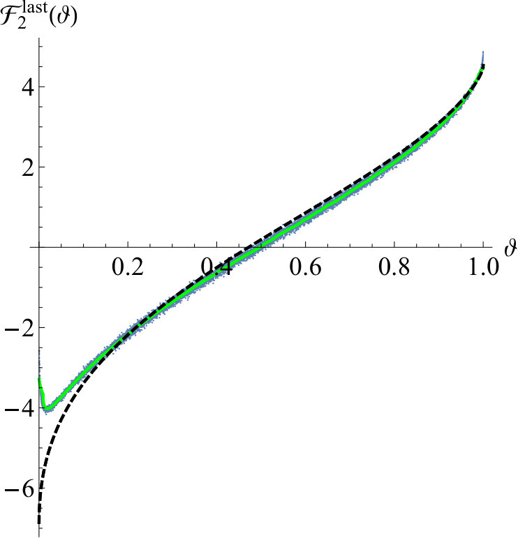 Figure 1
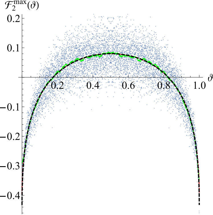 Figure 2
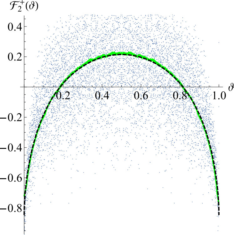 Figure 3
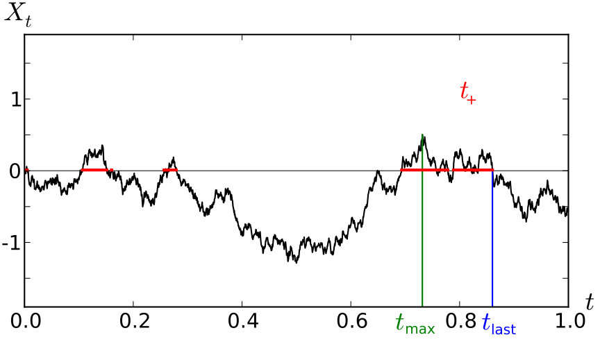 Figure 1
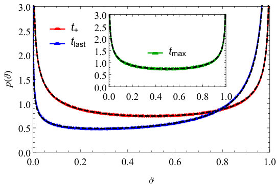 Figure 5
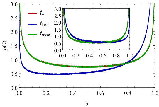 Figure 6
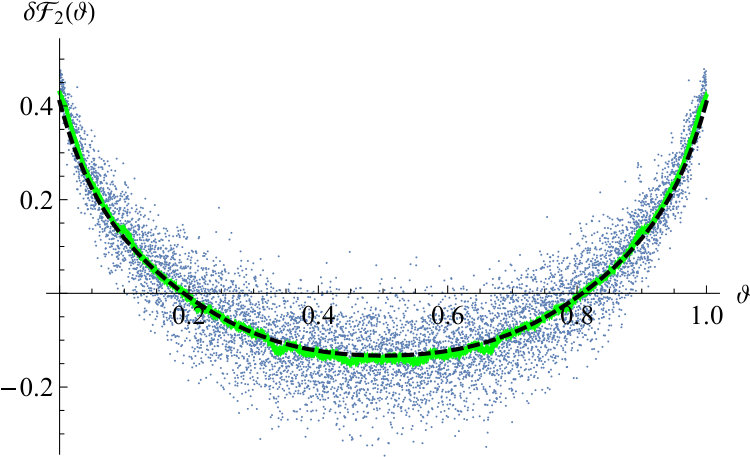 Figure 7
Peer Reviews
No public reviews on file for this paper yet. If you reviewed it on a platform where reviews are public (OpenReview, ICLR, NeurIPS, ICML), you can paste yours below so the community can read it here.
Videos
No videos yet. Explain this paper in a talk, walkthrough, or lecture? Add one.
Generalized arcsine laws for fractional Brownian motion
Tridib Sadhu
Tata Institute of Fundamental Research, Mumbai 400005, India.
Mathieu Delorme
Kay Jörg Wiese
Laboratoire de Physique Théorique, Département de Physique de l’ENS, Ecole Normale Supérieure, 24 rue Lhomond, 75005 Paris, France.
CNRS; PSL Research University; UPMC Univ. Paris 6, Sorbonne Universités.
Abstract
The three arcsine laws for Brownian motion are a cornerstone of extreme-value statistics. For a Brownian starting from the origin, and evolving during time , one considers the following three observables: (i) the duration the process is positive, (ii) the time the process last visits the origin, and (iii) the time when it achieves its maximum (or minimum). All three observables have the same cumulative probability distribution expressed as an arcsine function, thus the name of arcsine laws. We show how these laws change for fractional Brownian motion , a non-Markovian Gaussian process indexed by the Hurst exponent . It generalizes standard Brownian motion (i.e. ). We obtain the three probabilities using a perturbative expansion in . While all three probabilities are different, this distinction can only be made at second order in . Our results are confirmed to high precision by extensive numerical simulations.
pacs:
05.40.Jc, 02.50.Cw, 87.10.Mn
The three arcsine laws for Brownian motion or more generally for discrete random processes Levy1940 ; FellerBook ; Morters2010 ; Yen2013 are celebrated properties of stochastic processes. For a Brownian starting from the origin, and evolving during time , one considers the following three observables (see Fig. 1): (i) the total duration when the process is positive, (ii) the last time the process visits the origin, and (iii) the time it achieves its maximum (or minimum). Remarkably, all three observables have the same probability distribution as a function of ,
[TABLE]
As the cumulative distribution contains an arcsine function, these laws are commonly referred to as the first, second and third arcsine law. These laws apply quite generally to Markov processes, i.e. processes where the increments are uncorrelated FellerBook . Their counter-intuitive form with a divergence at and has sparked a lot of interest, and they are considered among the most important properties of stochastic processes. Recent studies led to many extensions, in constrained Brownian motion Majumdar2008 ; Bouchaud2008 ; Randon2007 , for general stochastic processes Majumdar2010 ; Schehr2010 ; HOCHBERG1994 ; Pitman1992 ; Carmona1994 ; Lamperti1958 , even in higher dimensions BARLOW1989 ; Bingham1994 ; Ernst2017 . The laws are realized in a plethora of real-world examples, from finance Dale1980 ; Baz2004 to competitive team sports Clauset2015 .
In this letter, we ask how these laws change for fractional Brownian motion (fBm) which is a generalization of standard Brownian motion preserving scale invariance as well as translation invariance, both in time and space. FBm was introduced in its final form by Mandelbrot and Van Ness MandelbrotVanNess1968 to describe time-series data in natural processes. It is defined as a Gaussian process , starting at zero, , with mean and covariance
[TABLE]
The parameter is the Hurst exponent. Standard Brownian motion corresponds to where the covariance reduces to . Unless , the process is non-Markovian, i.e. its increments are not independent. For they are positively correlated, while for they are anti-correlated. This non-Markovian nature makes a theoretical analysis of fBm difficult, and only few exact results are available in the literature Molchan1999 ; KrugKallabisMajumdarCornellBraySire1997 ; Guerin2016 .
FBm is important as it successfully models a variety of natural processes Decreusefond98 : a tagged particle in the single-file () (KrapivskyMallickSadhu2015, ; SadhuDerrida2015, ), the integrated current in diffusive transport () SadhuDerrida2016 , polymer translocation through a narrow pore () ZoiaRossoMajumdar2009 ; DubbeldamRostiashvili2011 ; PalyulinAlaNissilaMetzler2014 , anomalous diffusion BouchaudGeorges1990 , values of the log return of a stock () Peters1996 ; CutlandKoppWillinger1995 ; Biagini2008 ; Sottinen2001 , hydrology () MandelbrotWallis1968 , a tagged monomer in a polymer () GuptaRossoTexier2013 , solar flare activity () Moreno2014 , the price of electricity in a liberated market () Simonsen2003 , telecommunication networks () Norros2006 , telomeres inside the nucleus of human cells () Burnecki2012 , or diffusion inside crowded fluids () Ernst2012 . Generalizing the three arcsine laws (1) to fBm thus has fundamental importance, as well as a multitude of potential applications.
Unlike for Brownian motion, the probabilities of the three observables , and are different. Using an expansion in , we derive them in the form:
[TABLE]
The pre-factors of the exponential are predicted using scaling arguments for and . The terms in the exponential are non-trivial, and finite over the full range of . We use the convention that the integral over each -function vanishes, which adjusts the normalization constants . To leading order we find
[TABLE]
The expression of was reported earlier DelormeWiese2015 ; DelormeWiese2016 ; DelormeWiese2016b ; DelormeThesis . The equality of and , and their difference from the vanishing is qualitatively seen in Fig. 2. We have no intuitive understanding of this coincidence.
A numerical estimation of the three probabilities is obtained using a discrete-time algorithm DiekerPhD for fBm of a given , which generates sample trajectories drawn from a Gaussian probability with covariance (2). The probabilities in figures 2 and 3 are obtained by averaging over sample trajectories, each with time steps.
Figure 2 shows that behaves markedly differently from the other two distributions; especially, it is asymmetric under the exchange . This can be seen in the scaling part of Eq. (4), where the exponent comes from the return probability to the starting point, while the survival exponent governs the divergence for . This asymmetry in exponents is reversed around , as seen in the inset of figure 2.
The analytical expressions for in Eqs. (3)–(5) are cumbersome; we will sketch the derivation for the simplest one, , below, while the remaining ones will be reported elsewhere SadhuWieseToBePublished .
Confirmation of our theoretical results comes from comparison with numerical simulations of the probabilities presented in Fig. 3. For a finer comparison we plot our theoretical results of in Fig. 4 alongside their extraction from numerical simulations. To illustrate our procedure, we use Eq. (3) to define
[TABLE]
Then, which contains all terms in the exponential in Eq. (3) except . One can improve this estimation by using that the sub-leading term in is odd in , to define
[TABLE]
A comparison of extracted from numerical simulations of with the theoretical result of is plotted in Fig. 4 for . The figure also contains the comparison for and . As one sees, the agreement between theory and numerical simulations is quite striking: remind that these are sub-sub leading corrections, almost indiscernable in Fig. 3. We note the much larger amplitude of . The latter also has the largest deviations from the theory, especially for . These deviations indicate the presence of sub-leading terms of order , or higher.
In Fig. 2 the probabilities and are hard to distinguish from each other. Their difference can analytically be seen only at second order in . To underline that these are distinct distributions, we show the difference in Fig. 5.
In the rest of this letter we sketch the derivation of formulas (3)–(5). We begin with the action which characterizes the probability of a fBm trajectory,
[TABLE]
Here is the co-variance given in Eq. (2). We use an expansion WieseMajumdarRosso2010 ; DelormeWiese2016 of the action around to take advantage of the Markov property of Brownian motion. One writes
[TABLE]
which leads to an expansion of the action Note1
[TABLE]
where and all expressions are regularized by an ultraviolet cutoff in time.
Our calculation for the probabilities is done in Laplace variables. One reason for this choice is that the space integrals appearing in perturbation theory are easier. A further advantage is that temporal convolutions become mere products in the conjugate Laplace-variables. The action (12) is written in Laplace variables DelormeWiese2016 using
[TABLE]
where is the Heaviside function, and the UV cutoff is related to by with the Euler constant. As an explicit example, let us consider the calculation of and its Laplace transform
[TABLE]
The quantity of interest is which yields
[TABLE]
Defining , one obtains the probability by taking the inverse transformation
[TABLE]
where denotes the imaginary part. This is proven from Eq. (15) via analytical continuation.
The calculation is simplest at order zero in , i.e, for a Brownian. Using Eqs. (12) and (14) one writes
[TABLE]
Here is the Laplace transform of the Brownian propagator, while is the propagator in presence of an absorbing wall at the origin. This yields
[TABLE]
Using the transform (16) one obtains the arcsine law (1).
Perturbative corrections to the probability are evaluated by following a similar procedure DelormeWiese2016 . Contributions at different orders in are represented by the diagrams in Fig. 6. The non-vanishing contributions at order come from the two diagrams and which like (17) are expressed in terms of the Brownian propagator. For example, the amplitude corresponding to diagram is
[TABLE]
where . This leads to the non-trivial power-law in Eq. (4) and a vanishing in Eq. (7).
At order , there are multiple diagrams which contribute to the probability . However, the only contributions to come from the two diagrams and in Fig. 6. After some tedious algebra, the net amplitude of the two diagrams reads
[TABLE]
Finally, is obtained using
[TABLE]
which follows from Eqs. (16) and (4) footnote2 . Integrals in Eq. (Generalized arcsine laws for fractional Brownian motion) converge for leading to the result shown in the middle of Fig. 4.
Similar calculations for the other two probabilities and are more involved. For example, in ten diagrams contribute to the power-law in Eq. (5); in addition there are seven diagrams which contribute to . All these terms need to be grouped with the appropriate repeated first-order diagrams to yield combinations which converge for . These calculations will be reported elsewhere SadhuWieseToBePublished .
To summarize: we calculated the probabilities (3)-(5) generalizing the three arcsine laws to fBm up to order , improved by incorporating the exact scaling results for and . Our numerical simulations confirm these highly non-trivial predictions accurately.
Most realizations of fBm found in practical applications fall within the range where our formulas yield high-precision predictions. Our approach further offers a systematic framework to obtain other analytical results for non-Markovian processes, of which very few are available so far.
Acknowledgements.
We thank J. Klamser, P. Krapivsky, S.N. Majumdar and A. Rosso for stimulating discussions, and PSL for support by grant ANR-10-IDEX-0001-02-PSL. This research was supported in part by ICTS (Code: ICTS/Prog-NESP/2015/10).
The reference list from the paper itself. Each links out to its DOI / PubMed record.
- 1(1) P. Lévy, Sur certains processus stochastiques homogènes , Compositio Mathematica 7 (1940) 283–339.
- 2(2) W. Feller, Introduction to Probability Theory and Its Applications , John Wiley & Sons, 1950.
- 3(3) P. Mörters and Y. Peres, Brownian Motion , Cambridge University Press, 2010.
- 4(4) Ju-Yi Yen and M. Yor, Paul Lévy’s arcsine Laws , Springer International Publishing, Cham, 2013.
- 5(5) S. N. Majumdar, J. Randon-Furling, M. J. Kearney and M. Yor, On the time to reach maximum for a variety of constrained Brownian motions , J. Phys. A 41 (2008) 365005.
- 6(6) S. N. Majumdar and J. P. Bouchaud, Optimal time to sell a stock in the Black-Scholes model: comment on ‘Thou shalt buy and hold’, by A. Shiryaev, Z. Xu and X. Y. Zhou , Quantitative Finance 8 (2008) 753–760.
- 7(7) J. Randon-Furling and S. N. Majumdar, Distribution of the time at which the deviation of a Brownian motion is maximum before its first-passage time , J. Stat. Mech. (2007) P 10008.
- 8(8) S. N. Majumdar, Universal first-passage properties of discrete-time random walks and Lévy flights on a line: Statistics of the global maximum and records , Physica A 389 (2010) 4299–4316.