An optimal $(\epsilon,\delta)$-approximation scheme for the mean of random variables with bounded relative variance
Mark Huber

TL;DR
This paper introduces an efficient $(\epsilon,\delta)$-approximation scheme for estimating the mean of random variables with bounded relative variance, matching optimal sample complexity without requiring higher moment bounds.
Contribution
It presents a simple, easy-to-implement approximation method that achieves optimal sample complexity for mean estimation under bounded relative variance.
Findings
Achieves optimal sample complexity of approximately $2c^2\epsilon^{-2}\ln(1/\delta)$ samples.
Does not require bounds on third or fourth moments.
Provides a practical scheme for randomized approximation in complex counting problems.
Abstract
Randomized approximation algorithms for many #P-complete problems (such as the partition function of a Gibbs distribution, the volume of a convex body, the permanent of a -matrix, and many others) reduce to creating random variables with finite mean and standard deviation such that is the solution for the problem input, and the relative standard deviation for known . Under these circumstances, it is known that the number of samples from the needed to form an -approximation that satisfies is at least . We present here an easy to implement -approximation that uses samples. This achieves the same optimal running…
Click any figure to enlarge with its caption.
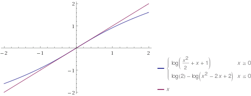 Figure 1
Peer Reviews
No public reviews on file for this paper yet. If you reviewed it on a platform where reviews are public (OpenReview, ICLR, NeurIPS, ICML), you can paste yours below so the community can read it here.
Videos
No videos yet. Explain this paper in a talk, walkthrough, or lecture? Add one.
Taxonomy
TopicsMarkov Chains and Monte Carlo Methods · Point processes and geometric inequalities · Statistical Methods and Inference
An optimal
-approximation scheme for the mean of random variables with bounded relative variance
Mark Huber
Abstract
Randomized approximation algorithms for many #P-complete problems (such as the partition function of a Gibbs distribution, the volume of a convex body, the permanent of a -matrix, and many others) reduce to creating random variables with finite mean and standard deviation such that is the solution for the problem input, and the relative standard deviation for known . Under these circumstances, it is known that the number of samples from the needed to form an -approximation that satisfies is at least . We present here an easy to implement -approximation that uses samples. This achieves the same optimal running time as other estimators, but without the need for extra conditions such as bounds on third or fourth moments.
1 Introduction
Suppose are iid with mean and variance . The relative standard deviation is and the relative variance is . Say the relative standard deviation is bounded by if
[TABLE]
Suppose and are unknown, but is known. Then the goal is to use as few as possible to find an estimate for that is an -randomized approximation, that is
[TABLE]
Suppose that an -randomized approximation requires
[TABLE]
samples for a constant and where the little-o notation refers to . Then call the scale factor of the algorithm.
In this work we present a simple algorithm that is both easy to implement and which achieves the optimal scale factor without any additional assumptions about the random variables such as bounded higher moments.
This basic problem arises often in randomized algorithms. For instance, problems for approximating the partition function of the Ising model [14], the permanent of a -matrix [17], the volume of a convex body [7, 18], the number of solutions to a DNF logical expression [16], the number of linear extensions of a poset [20, 11], and many more all have this problem as a subproblem. Any improvement in the ability to deal with this basic problem directly translates into better approximation algorithms for all of these problems.
This problem has a long history, stretching back to Nemirovsky and Yudin [23] who used the median-of-means estimator in the context of stochastic optimization. Jerrum, Valiant, and Vazirani [16] developed a similar estimator for the purposes of creating randomized approximation schemes for #P complete problems. By 1999 [1], this method was in wide use for online algorithms. Hsu and Sabato [9, 10] analyzed the basic median-of-means estimator and proved that it had a scale factor of 121.5 for small enough .
Catoni [4] greatly advanced the area by presenting an approximation that used an -estimator. This was not an -randomized approximation algorithm, rather it gave a confidence bound based on the samples and specific values of the parameters used in the estimate. While it could bound the confidence interval for the estimate based on the parameters and the unknown and for , there seems to be no way of setting the parameters ahead of time for given and without some additional information. Certainly no such method was given in [4].
Devroye et. al. [6] showed that if the kurtosis of the random variables is bounded above, then the optimal scale factor could be attained with a simpler estimator. Unfortunately, in order to run their algorithm, the user needed this upper bound on the kurtosis. Bounding the kurtosis can be much more challenging mathematically than bounding the variance. Minsker and Strawn [21] returned to the original median-of-means estimator. When the random variables have bounded third moment, the Berry-Esseen Theorem can be used to show quick convergence to normality, and they showed that this gave the simple median-of-means algorithm a scale factor of 4.5. As with the Devroye et. al. method, this requires that the bound on the third moment be given explicitly before the algorithm can be used.
The approach here takes the Catoni -estimator in a new direction. There is no unique approach to getting the extra information required to turn the Catoni -estimator into an -approximation. One approach is to use a two-step process that works as follows. Before running the -estimator, first generate a weaker estimate that is an randomized approximation to . Then use this estimate to set the parameters of the Catoni -estimator to give an output that is provably an -approximation.
While this two-step process works, it (like all -estimators) requires finding the root of a nonlinear equation. Analysis of the number of steps needed to get an close approximation to the root was not done in [4], and would need to be accomplished before the running time of the method is known.
Previous algorithms either had too large a scale factor, required rootfinding, or required knowledge of higher moments. The new method presented here solves all these difficulties.
- •
It achieves the optimal scale factor .
- •
No rootfinding step is required. Instead, first a function is randomly chosen by some initial samples, and then the final estimator is a sample average this random function applied to new data.
- •
No bound on higher moments is necessary. In fact, even if the second moment is the highest moment that exists for the random variables, the new method is still an -randomized approximation.
Our main result concerning this new method is as follows.
Theorem 1**.**
Let with and satisfying For , there exists an -randomized approximation algorithm that uses samples where
[TABLE]
This constant in the leading order term is the best possible.
Theorem 2**.**
Given and positive, let be an -randomized algorithm for all distributions with and satisfying . Then
[TABLE]
The remainder of the paper is organized as follows. The next section describes the two-step algorithm and proves correctness for each step. Section 3 then shows the lower bound on the number of samples needed, and Section 4 considers several of the applications mentioned in the introduction in more detail.
2 The Algorithm
Define the function as follows.
[TABLE]
This function was used in [4] as part of the -estimator.
For , the value of is approximately (see Figure 1.) For greater than 1 in magnitude, the value of becomes close to 0. For a constant , is a scaled version of that is close to for .
Suppose that is an initial estimate for . Then
[TABLE]
has mean but is also susceptible to outliers in the distribution. By replacing this with
[TABLE]
the value of will be close to when , but always has a light-tailed distribution because of the logarithm function.
The algorithm proceeds as follows. The first step uses a median-of-means approach to find that is a approximation of . Given that the first step did not fail, the next step then uses the sample average of the variables to create the final estimate that is an approximation. The chance that either step fails is at most .
The first step is to construct a median-of-means estimator for [16]. Let and . Let have the distribution of the sample average of independent draws from . Draw independently, and let . 2. 2.
Let , and . Draw independently. For all , let
[TABLE]
Set .
2.1 The first step of the algorithm
The first step of the algorithm is the powering method of Jerrum, Valiant, and Vazirani [16] applied to the sample averages. This technique was also used in [1], and later referred to as the median-of-means method [9]. These authors did not attempt to optimize the constants in their arguments, and so we repeat the proof here so we can see exactly how the choice of constant enters into the failure bound.
Suppose that we have random variables whose relative standard deviation is at most . What is the chance that the median of draws from the random variable falls into ?
To answer this question, first consider the probability that a beta distributed random variable with both parameters equal to an integer falls into a subinterval of .
Lemma 1**.**
Let denote a random variable with density . For any with ,
[TABLE]
Proof.
Density is symmetric about its unique local maximum at , so
[TABLE]
Note . Let Then , and , so the function lies below its tangent line at . That is,
[TABLE]
Then
[TABLE]
Using Stirling’s formula to give completes the proof. ∎
Lemma 2**.**
Let be iid with mean and variance at most where . Then
[TABLE]
Proof.
By Chebyshev’s inequality,
[TABLE]
Let and . Construct a uniform random variable over as follows. If , then let . If , let . Finally, if , then let . Note that
[TABLE]
The median of iid uniform random variables is well known to have a beta distribution: . So the previous lemma can be used to state
[TABLE]
∎
Hence the failure probability is going down exponentially at rate Now for an integer , consider iid, and
[TABLE]
Then and
In particular, for , and , To take the median of draws of the sample average of draws from the takes samples.
Lemma 3** (Median-of-means).**
Suppose are as in (1). For let be distributed as . Let Let then
[TABLE]
Proof.
Just set in the previous lemma to get a rough minimum for the bound. ∎
Now suppose that instead of bounding , we wish to bound . The next lemma shows how to build a biased estimate where from an estimate with relative error at most .
Lemma 4**.**
Suppose is an estimate for with . Then has .
Proof.
The proof follows from simplifying the appropriate inequalities. ∎
This is why in the first step of the algorithm, the estimate found from median-of-means is divided by before moving to the next step.
2.2 The second step of the algorithm
To analyze this step, it helps to have two new functions that upper and lower bound .
[TABLE]
Lemma 5**.**
For all ,
[TABLE]
Proof.
First consider . These are equal when , so suppose . Exponentiating gives
[TABLE]
therefore the inequality holds. The other inequality is shown similarly. ∎
Now set
[TABLE]
By the previous lemma, for all .
Lemma 6**.**
Denote . Then
[TABLE]
Proof.
Take a Chernoff bound [5] style approach. Since and is a strictly increasing function,
[TABLE]
First consider the expression inside the mean in the numerator. Setting gives
[TABLE]
Since and , we have
[TABLE]
Note
[TABLE]
Next use to state
[TABLE]
Since , and ,
[TABLE]
Similarly, using ,
[TABLE]
Note .
Putting this together with the term gives
[TABLE]
∎
Note that at the end of Step 1 of the algorithm, , which means , and
Lemma 7**.**
Denote . Then
[TABLE]
Proof.
The proof is similar to the previous lemma: first multiply by and exponentiate to get
[TABLE]
and the rest of the proof is the same as the previous lemma. ∎
Putting these results together gives the following.
Lemma 8**.**
For and ,
[TABLE]
Proof.
Apply the previous lemma using ∎
Theorem 1 immediately follows.
3 Lower bound on the number of samples
Begin with a rephrasing of Proposition 6.1 from [4].
Lemma 9**.**
Let be any estimator of the mean of iid random variables. Let and . Then it holds that either or for .
In other words, for any estimator of the mean for normal random variables, there is either a higher chance that the estimate is in the upper tail than for the sample average, or there is a higher chance that the estimate falls in the lower tail than the sample average does. Note that for , then . Let . From the scaling properties of normal random variables,
[TABLE]
Since for all , we need only bound one tail of the normal.
Lemma 10**.**
Let and satisfy where . Then
[TABLE]
Proof.
Gordon [8] showed that for ,
[TABLE]
Without the factor, the right hand side equals when . Since we have . Also, is a decreasing function, so
[TABLE]
Solving gives
[TABLE]
as desired. ∎
Putting then gives Theorem 2.
4 Applications
Jerrum, Valiant, and Vazirani [16] showed that for a large class of self-reducible problems, the ability to sample from a density in polynomial time leads to an -randomized approximation scheme for the normalizing constant of the unnormalized density. Since finding that normalizing constant is often a #P-complete problem, this has been used in many settings. Each of these leads to a problem such as that considered here where a random variable has mean equal to the target with bounded relative standard deviation. This method was expanded to more examples later by Jerrum and Sinclair [15].
The idea is as follows. Suppose that the goal is to find which is the size of a set (either number of elements for a finite set or the Lebesgue measure for .) Suppose that we can find a sequence of decreasing sets where is known. If each of the sets represents an instance of the original problem (perhaps with a different input), the problem is self-reducible. If there is an efficient method for generating samples uniformly from the , then for each , let , and let be the percentage of values that fall into . Then
[TABLE]
so let be the unbiased product estimator for .
Then
[TABLE]
Let . Then has a Bernoulli distribution with mean and variance . As the sample average of iid draws from , has mean and variance . Then
[TABLE]
so if for all , using gives
[TABLE]
There are different each requiring samples, therefore are needed to generate one value of . From the above the variance is for large . Hence for large (such as ) using the algorithm presented here has the total number of samples needed for an -approximation is (to leading order) , with the 2 being the optimal value of the constant.
4.1 Linear extensions of a poset
For a direct application of this process, consider the problem of counting the number of linear extensions of a partially ordered set (poset). A poset on objects is an ordering with three properties. Let . First, . Second, if and , then . Third, if and , then . A linear extension of the poset is a permutation such that .
Brightwell and Winkler [2] showed that counting the number of linear extensions of an arbitrary poset is a #P-complete problem. Finding the number of linear extensions has applications in nonparametric statistics [22].
A sequence of results [19, 20, 3, 11] culminated in an method for generating samples uniformly from the set of linear extensions. To convert this method into a method for approximately counting the number of linear extensions, use self-reducibility.
Let be any element of which is not preceded by another element in the set. Then an easy Markov chain argument gives that the probability that a uniformly chosen linear extension has is at least . Fixing in the permutation leaves a linear extension problem of size . So the methods of this section can be applied with and . Hence (to first order) samples are needed to give an -approximation to the number of linear extensions.
4.2 Permanent of a -matrix
Let be the set of permutations on . Then the permanent of a matrix with entries is
[TABLE]
Calculating the permanent exactly was shown by Valiant [25] to be a #P-complete problem.
Note that if , then the only permutations that contribute to the sum have for all . So the permanent is the normalizing constant of the distribution over with unnormalized density
Jerrum, Sinclair, and Vigoda [17] developed a polynomial time algorithm for approximately sampling from the density . As with the previous problem of linear extensions, for such a problem on permutations there exists a value such that . This can then be used with the basic self-reducibility process to get an -approximation for the permanent. Without going into details (as the method of [17] for approximation was more complex than the basic approach) the result is the same as for linear extensions: use of the methods of this paper immediately reduces the constant in the leading term down to the optimal value.
4.3 Gibbs distributions
These distributions arise in statistical physics and other applications.
Definition 1**.**
is a Gibbs distribution with parameter over finite state space if there exists a Hamiltonian function such that for ,
[TABLE]
where is called the partition function of the distribution.
A famous example of a Gibbs distribution is the Ising model [13], where the state space consists of labellings of the nodes of a graph by either 0 or 1, and In [14] finding the partition function of the ferromagnetic Ising model (where ) was shown to be a #P-complete problem for general graphs, but that same work showed how to generate (approximately) samples from the distribution in time polynomial in the size of the graph.
Typically it is easy to find for these problems. For the Ising model, . In [24] it was shown how to build an estimate for using samples from where the ratio was bounded. In [12], it was shown how to build two random variables and such that and each had relative variance bounded above by .
Let for . If
[TABLE]
then
[TABLE]
Then it is straightforward to show that satisfies
[TABLE]
thereby giving an -approximation that (to leading order) requires samples to estimate the partition function value.
The reference list from the paper itself. Each links out to its DOI / PubMed record.
- 1[1] N. Alon, Y. Matias, and M. Szegedy. The space complexity of approximating the frequency moments. J. Comput. Syst. Sci. , 58:137–147, 1999.
- 2[2] G. Brightwell and P. Winkler. Counting linear extensions. Order , 8(3):225–242, 1991.
- 3[3] R. Bubley and M. Dyer. Faster random generation of linear extensions. Disc. Math. , 201:81–88, 1999.
- 4[4] O. Catoni. Challenging the empirical mean and empirical variance: A deviation study. Ann. Inst. H. Poincaré Probab. Statist. , 48:1148–1185, 2012.
- 5[5] H. Chernoff. A measure of asymptotic efficiency for tests of a hypothesis based on the sum of observations. Ann. of Math. Stat. , 23:493–509, 1952.
- 6[6] L. Devroye, M. Lerasle, G. Lugosi, and R.I. Oliveira. Sub-gaussian mean estimators. Ann. Statist. , 44:2695–2725, 2016.
- 7[7] M. Dyer, A. Frieze, and R. Kannan. A random polynomial-time algorithm for approximating the volume of convex bodies. J. Assoc. Comput. Mach. , 38(1):1–17, 1991.
- 8[8] R.D. Gordon. Values of Mills’ ratio of area to bounding ordinate of the normal probability integral for large values of the argument. Annals of Mathematical Statistics , 12:364–366, 1941.