TL;DR
This paper explores how the clustering structure of graphs can be exploited to improve the efficiency of estimating Personalized PageRank for many node pairs, especially in large networks and distributed computing environments.
Contribution
It introduces an enhanced PPR estimation algorithm and demonstrates how leveraging clustering reduces computational complexity in both centralized and distributed settings.
Findings
Joint estimation is easier with high clustering.
Clustering-aware task assignment improves distributed computation efficiency.
Enhanced Bidirectional-PPR improves multi-pair estimation performance.
Abstract
Personalized PageRank (PPR) is a measure of the importance of a node from the perspective of another (we call these nodes the and the , respectively). PPR has been used in many applications, such as offering a Twitter user (the source) recommendations of who to follow (targets deemed important by PPR); additionally, PPR has been used in graph-theoretic problems such as community detection. However, computing PPR is infeasible for large networks like Twitter, so efficient estimation algorithms are necessary. In this work, we analyze the relationship between PPR estimation complexity and clustering. First, we devise algorithms to estimate PPR for many source/target pairs. In particular, we propose an enhanced version of the existing single pair estimator that is more useful as a primitive for many pair estimation. We then…
Click any figure to enlarge with its caption.
 Figure 1
 Figure 2
 Figure 3
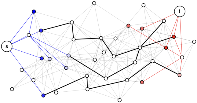 Figure 4
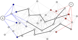 Figure 5
 Figure 6
 Figure 7
 Figure 8
 Figure 9
 Figure 10
 Figure 11
 Figure 12
 Figure 13
 Figure 14
 Figure 15
 Figure 16
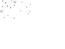 Figure 17
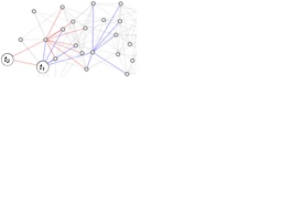 Figure 18
 Figure 19
 Figure 20
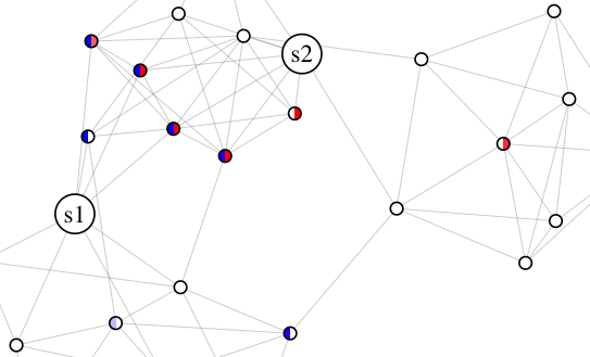 Figure 21
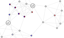 Figure 22
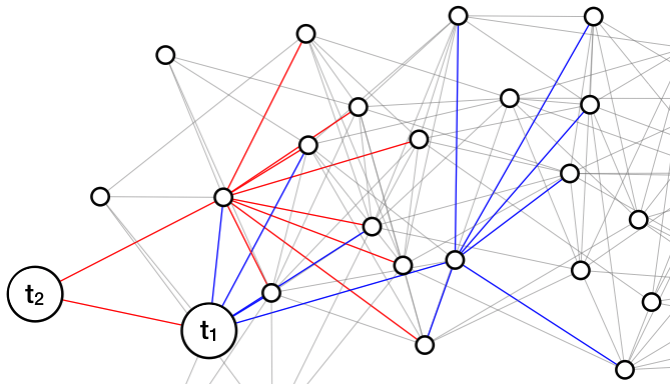 Figure 23
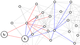 Figure 24
 Figure 25
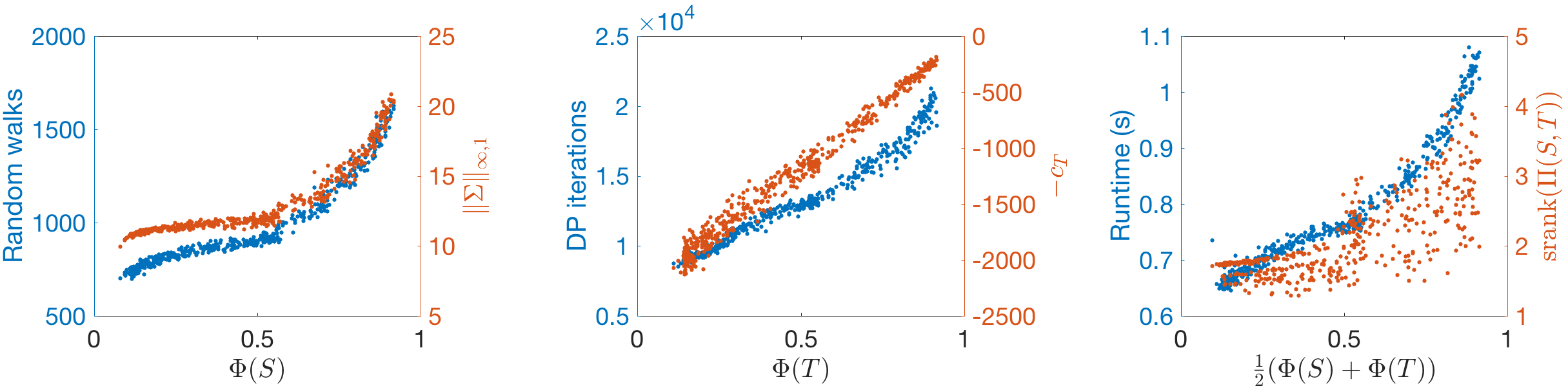 Figure 26
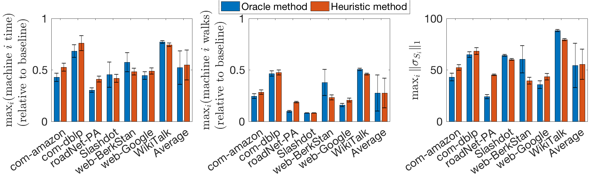 Figure 27
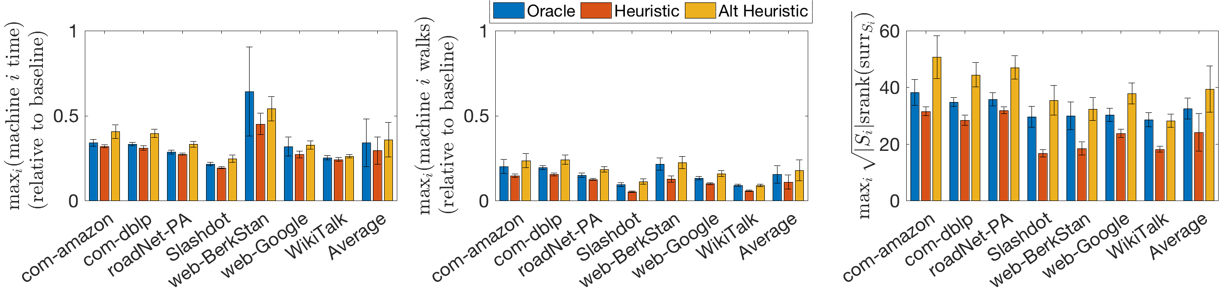 Figure 28
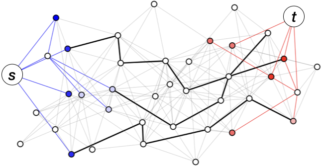 Figure 29
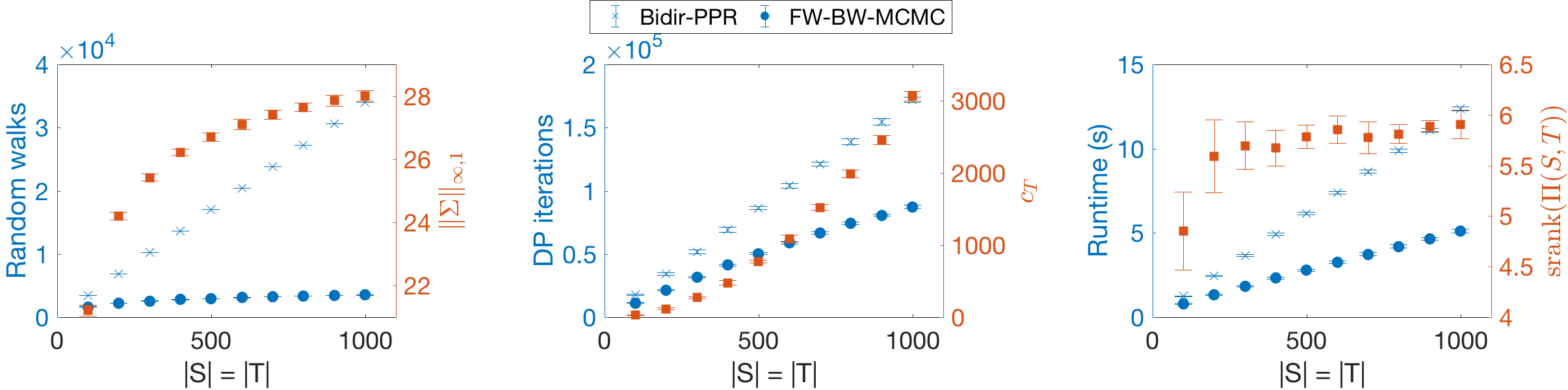 Figure 30
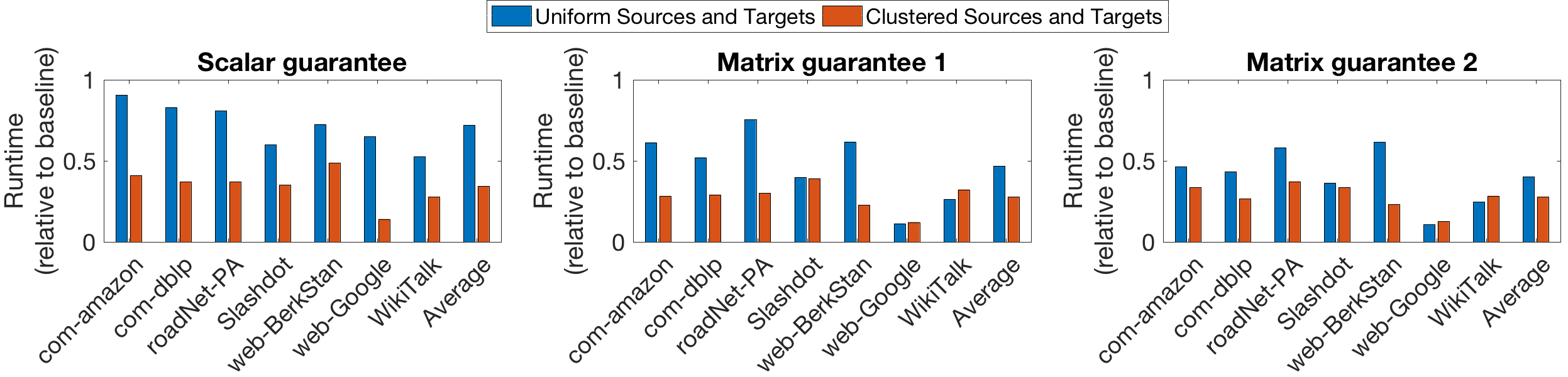 Figure 31
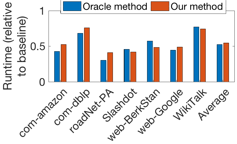 Figure 32
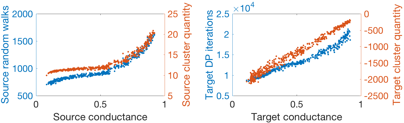 Figure 33
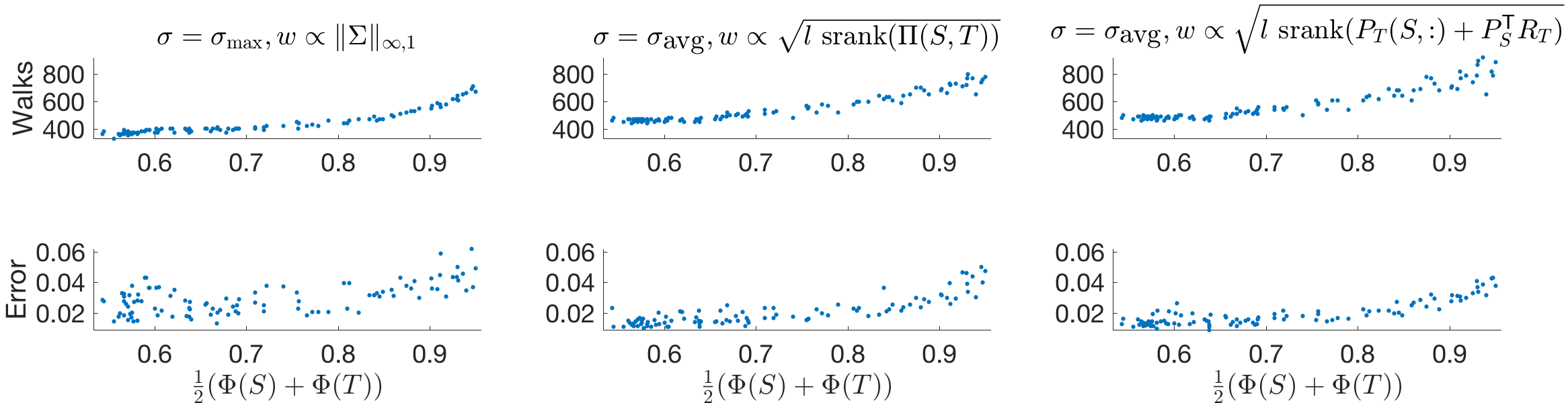 Figure 34
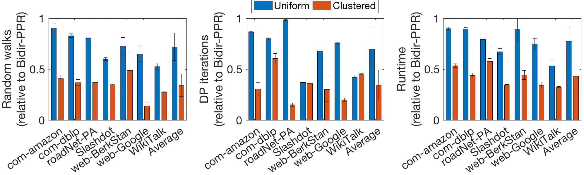 Figure 35
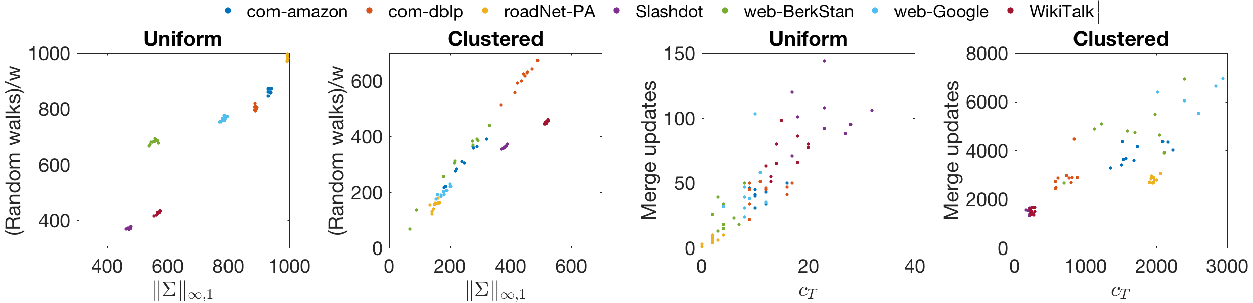 Figure 36
 Figure 37
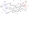 Figure 38
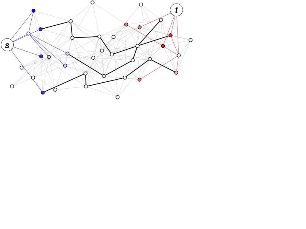 Figure 39
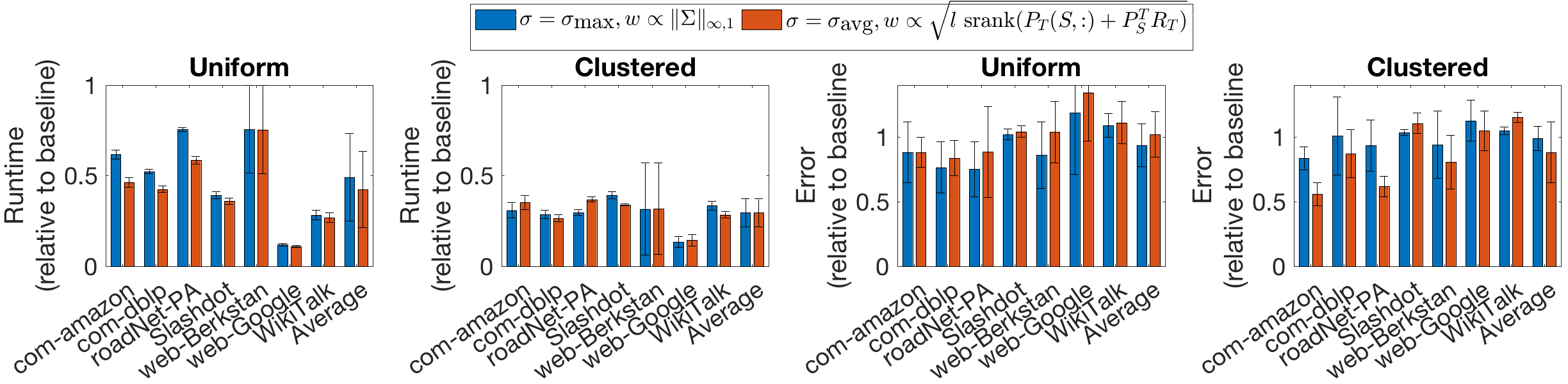 Figure 40
| Notation | Defined in | Description |
| Section 2 | Global PageRank vector, PPR vector for | |
| Section 4 | Output vectors of Algorithm 1 (forward DP); satisfy (5) | |
| Section 4 | Starting distribution for walks in FW-BW-MCMC; | |
| Section 4 | Upper bound on at conclusion of Algorithm 1 | |
| Section 4 | Output vectors of Algorithm 2 (backward DP); satisfy (6) | |
| Section 4 | Upper bound on at conclusion of Algorithm 2 | |
| Section 5.1.1 | Matrix with rows (subscript omitted at times) | |
| Section 5.1.1 | Source clustering quantity; see (12) | |
| Section 5.1.2 | Target clustering quantity; see (22) | |
| Section 5.2 | Stable rank of matrix ; | |
| Section 5.2 | Matrices containing , , , , resp. | |
| Section 5.2 | Matrix containing | |
| Section 5.2 | Starting distributions for walks in matrix estimators; see (27) | |
| Section 6.1.1 | Conductance of ; see (30) | |
| Section 7 | Vector with |
| Dataset | Description | ||
|---|---|---|---|
| com-Amazon | Amazon co-purchasing | 334863 | 925872 |
| com-dblp | Scientific co-authorship | 317080 | 1049866 |
| roadNet-PA | Roads in Pennsylvania | 1087532 | 1541514 |
| Slashdot | Friendships on technology news site | 71307 | 912381 |
| web-BerkStan | berkley.edu, stanford.edu web graph | 334857 | 4523232 |
| web-Google | Partial web crawl | 434818 | 3419124 |
| Wiki-Talk | Friendships among Wikipedia editors | 111881 | 1477893 |
| Graph | Algorithm | DP time (ms) | MC time (ms) | Error | ||||
| Direct-ER | FW-BW-MCMC-Prac | 10.61 | 7.63 | 0.075 | ||||
| Direct-ER | Bidirectional-PPR | N/A | 6.94 | 7.52 | 0.072 | |||
| Direct-SBM | FW-BW-MCMC-Prac | 15.43 | 7.08 | 0.052 | ||||
| Direct-SBM | Bidirectional-PPR | N/A | 10.19 | 12.01 | 0.061 | |||
| com-amazon | FW-BW-MCMC-Prac | 22.55 | 22.54 | 0.12 | ||||
| com-amazon | Bidirectional-PPR | N/A | 22.13 | 22.21 | 0.11 | |||
| com-dblp | FW-BW-MCMC-Prac | 20.27 | 20.31 | 0.12 | ||||
| com-dblp | Bidirectional-PPR | N/A | 20.03 | 19.65 | 0.11 | |||
| roadNet-PA | FW-BW-MCMC-Prac | 55.04 | 56.58 | 0.11 | ||||
| roadNet-PA | Bidirectional-PPR | N/A | 53.19 | 55.96 | 0.10 | |||
| Slashdot | FW-BW-MCMC-Prac | 3.08 | 3.38 | 0.10 | ||||
| Slashdot | Bidirectional-PPR | N/A | 3.30 | 4.03 | 0.11 | |||
| web-BerkStan | FW-BW-MCMC-Prac | 11.13 | 11.02 | 0.12 | ||||
| web-BerkStan | Bidirectional-PPR | N/A | 8.40 | 8.42 | 0.12 | |||
| web-Google | FW-BW-MCMC-Prac | 23.33 | 22.83 | 0.11 | ||||
| web-Google | Bidirectional-PPR | N/A | 26.07 | 22.29 | 0.11 | |||
| WikiTalk | FW-BW-MCMC-Prac | 4.40 | 3.99 | 0.11 | ||||
| WikiTalk | Bidirectional-PPR | N/A | 5.84 | 5.10 | 0.11 |
Peer Reviews
No public reviews on file for this paper yet. If you reviewed it on a platform where reviews are public (OpenReview, ICLR, NeurIPS, ICML), you can paste yours below so the community can read it here.
Code & Models
Videos
No videos yet. Explain this paper in a talk, walkthrough, or lecture? Add one.
On the role of clustering in Personalized PageRank estimation
Daniel Vial
University of Michigan
and
Vijay Subramanian
University of Michigan
Abstract.
Personalized PageRank (PPR) is a measure of the importance of a node from the perspective of another (we call these nodes the target and the source, respectively). PPR has been used in many applications, such as offering a Twitter user (the source) recommendations of who to follow (targets deemed important by PPR); additionally, PPR has been used in graph-theoretic problems such as community detection. However, computing PPR is infeasible for large networks like Twitter, so efficient estimation algorithms are necessary.
In this work, we analyze the relationship between PPR estimation complexity and clustering. First, we devise algorithms to estimate PPR for many source/target pairs. In particular, we propose an enhanced version of the existing single pair estimator Bidirectional-PPR that is more useful as a primitive for many pair estimation. We then show that the common underlying graph can be leveraged to efficiently and jointly estimate PPR for many pairs, rather than treating each pair separately using the primitive algorithm. Next, we show the complexity of our joint estimation scheme relates closely to the degree of clustering among the sources and targets at hand, indicating that estimating PPR for many pairs is easier when clustering occurs. Finally, we consider estimating PPR when several machines are available for parallel computation, devising a method that leverages our clustering findings, specifically the quantities computed in situ, to assign tasks to machines in a manner that reduces computation time. This demonstrates that the relationship between complexity and clustering has important consequences in a practical distributed setting.
1. Introduction
Many systems, ranging from social networks to financial markets to the human brain, can be represented as graphs. When analyzing such systems, questions regarding the importance of nodes and the relationships between them arise. Which nodes are most influential, globally and locally? From the perspective of a given node, which nodes are important, and which nodes consider the given node to be important? How can these notions be quantified?
PageRank and Personalized PageRank (PPR) can help answer such questions. PageRank is a measure of the importance or centrality of a target node; PPR “personalizes” this measure to the perspective of a source node. Proposed to rank Internet search results (Page et al., 1999), and later to personalize these rankings (Haveliwala, 2002), PageRank and PPR have been used in applications such as recommending Twitter followers (Gupta et al., 2013) and YouTube videos (Baluja et al., 2008), as well as “beyond the web” (Gleich, 2015), in fields such as bioinformatics (Morrison et al., 2005; Freschi, 2007). In graph theory, PPR has been used as a primitive for tasks such as detecting communities near a seed node (Andersen et al., 2006) and assessing similarity between graphs (Koutra et al., 2013).
The widespread use of PageRank and PPR can be attributed to the notion of relational “importance” they convey, as well as the simplicity of the model from which they are derived. However, the scale of modern networks often makes them difficult (or impossible) to compute. As such, strategies for efficient estimation of PageRank and PPR are necessary.
Our contributions: In this work, we analyze the relationship between clustering and PPR estimation complexity. In particular, we devise algorithms to estimate PPR for many source/target pairs, and we show that the complexity of these methods decreases with increased clustering among the sources and targets at hand. To demonstrate the consequences of our findings, we consider a distributed setting in which this relationship between complexity and clustering can be leveraged to design more efficient algorithms. More specifically, our contributions are as follows:
- (1)
In Section 4, we propose an enhancement of Bidirectional-PPR (Lofgren et al., 2016), the state-of-the-art PPR estimator for a single source/target pair. As the name suggests, Bidirectional-PPR estimates PPR in two stages: random walks forward from the source node and dynamic programming (DP) backward from the target node. Our algorithm, called FW-BW-MCMC, adds a DP stage forward from the source that allows it to serve as a primitive in the many pair setting. In Appendix A, we establish similar guarantees to those for Bidirectional-PPR. 2. (2)
In Section 5, we use FW-BW-MCMC as a primitive to estimate PPR for many pairs, proposing methods that accelerate the naive scheme of separately sampling random walks for each source and separately running DP for each target. For the sources, we show the forward DP allows random walk samples to be shared, decreasing the number of samples required. For the targets, we define a new iterative update for the backward DP, which eliminates repeated computations that may occur when treating each target separately. Using these ideas, we devise an algorithm with accuracy guarantees on each scalar estimate, and two algorithms with accuracy guarantees on the matrix containing all estimates. Across a diverse set of graphs, our methods are roughly 1.1 to 9.3 times faster than baseline methods (Fig. 1(a)). 3. (3)
We show analytically in Section 5 and empirically in Section 6 that the accelerations offered by our algorithms are most significant when the sources and targets are each clustered together in the graph, i.e. PPR estimation is “easier” when clustering occurs. For example, our algorithms typically accelerate baseline methods by factors of 3-4 when clustering occurs (Fig. 1(a)). More specifically, we prove the number of random walks for the sources and the number of DP iterations for the targets scale with quantities that describe clustering among the sources and targets, respectively; we find empirically that these clustering quantities scale with a more traditional clustering quantity, conductance (Fig. 1(b)). Also, while these clustering quantities are difficult to analyze in general, we provide analytical results for the stochastic block model, the prototypical model for networks with community structure. 4. (4)
Finally, in Section 7, we demonstrate an application of our results, showing that our findings can be used to devise efficient algorithms when estimating PPR in a distributed setting. Specifically, we show that quantities computed during the forward DP can be used to predict the random walk sampling time for different assignments of tasks to machines, and we propose a natural but heuristic method to compute an assignment that (locally) minimizes this time. At a high level, our method “learns” the clustering structure present at runtime; empirically, this learning is quite successful, in the sense that our method performs nearly as well as an oracle method that knows the clustering structure a priori (Fig. 1(c)).
The remainder of the paper is organized as follows. We begin with preliminaries and related work in Sections 2 and 3, respectively. Sections 4-7 follow the outline above. We close in Section 8.
2. Preliminaries
We begin with some preliminary definitions. Let be a directed graph, and define . For , let denote ’s outgoing neighbors, and let denote the out-degree of . For simplicity, we assume . Similarly define and as ’s incoming neighbors and in-degree. Finally, let denote the adjacency matrix of , let be the diagonal matrix with , and define .
PageRank (Page et al., 1999) is the stationary distribution of the Markov chain with transition matrix , where and denotes the all ones vector of length . In words, this chain is a random walk on for which, with probability at each step, the random walker “jumps” to a uniform node, rather than following the walk. Let us denote this chain by . Clearly, is irreducible and aperiodic, as . Assuming is finite, positive recurrence follows, so exists, is unique, and satisfies
[TABLE]
It is by (1) that PageRank gives a measure of “importance”: we consider important when is large, which occurs when is visited often on the chain .
We will henceforth refer to PageRank as global PageRank to distinguish it from the generalization to PPR. Formally, PPR is the stationary distribution of the Markov chain with transition matrix . Here is a nonnegative vector that sums to 1; hence, it yields a distribution on the jump locations, generalizing the uniform jumps of global PageRank. This gives an interpretation like (1), while also accounting for the preference on jump locations given by .
There are two important mathematical viewpoints of PPR that serve as the foundation for many estimation techniques; we will make use of both in the sections that follow. The first viewpoint is linear algebraic. Here we let denote the stationary distribution as a row vector. By global balance, satisfies ; solving for (and assuming is normalized to sum to 1) gives
[TABLE]
Note this immediately suggests estimating PPR by computing the first terms of the summation. The second PPR viewpoint is probabilistic. Denoting by the Markov chain with transition matrix , and letting , (Athreya and Stenflo, 2003) shows
[TABLE]
which again suggests estimation techniques; in this case, using Markov chain Monte Carlo (MCMC). We note this viewpoint is closely related to exact sampling (Propp and Wilson, 1996) and Doeblin chains (Athreya and Stenflo, 2003; Meyn and Tweedie, 2012).
Often, we let for some , where satisfies . In such a case, we denote PPR as and the transition matrix as . In fact, using (2), one can show
[TABLE]
Due to (4), many PPR estimation algorithms focus on estimating , from which extensions to estimating naturally follow; we focus on this as well throughout the paper.
Finally, we argue existence and uniqueness of PPR is not a concern. Indeed, the PPR Markov chain is aperiodic (since ), so to guarantee existence and uniqueness, we need only verify irreducibility. For this, let V_{s}=\{v\in V:\textrm{\existssvG}\}, so that , s.t. (we can jump from to , then reach from ). Hence, if is not irreducible, we can define a modified chain with states that is irreducible and obtain the stationary distribution for this chain. We can then set – intuitively, if cannot reach , is not “important” to , so its PPR should be zero. Given this simple fix, we assume existence and uniqueness of PPR.
3. Related Work
Before proceeding, we discuss some existing PPR estimation algorithms. Broadly speaking, these can be organized hierarchically: first, those that estimate the entire PPR matrix ; second, those that estimate a single row or column of this matrix, or its column sums (i.e. global PageRank); and third, those that estimate a single entry .
At the first level, several algorithms have been proposed to accelerate the power iteration or matrix inversion in (2). To accelerate the power iteration, (Jeh and Widom, 2003) provides a decomposition that allows a single row of the PPR matrix to be estimated using previously-computed rows; hence, this yields a procedure of first computing a small number of rows and then using these to estimate other rows. To obtain less costly matrix inversions, several works, e.g. (Tong et al., 2008; Shin et al., 2015), have leveraged structural assumptions of the graph at hand. For example, Tong et al. in (Tong et al., 2008) propose a decomposition of into a block diagonal matrix and ; for graphs like social networks, can be extremely sparse. From the probabilistic viewpoint (3), (Fogaras et al., 2005) gives an algorithm to estimate any entry of the PPR matrix at runtime using a precomputed database of random walk samples.
At the second level, algorithms include the dynamic programming methods in (Andersen et al., 2006) and (Andersen et al., 2008) that estimate a row and a column of the PPR matrix, respectively; both can be viewed as localized versions of the power iteration in (2). The algorithm in (Andersen et al., 2006) yields and error guarantees on the row estimate with complexity , while (Andersen et al., 2008) gives an guarantee on the column estimate with complexity . We make use of these algorithms in our methods and will discuss them in more detail in Section 4. We also note the approach in (Andersen et al., 2006; Andersen et al., 2008) is closely related to work by Lee and co-authors (Lee et al., 2013, 2014a, 2014b) that focuses on estimation of the stationary distribution of countable state-space Markov chains, as well as estimation in the context of general linear systems. From the probabilistic viewpoint, an important work is (Avrachenkov et al., 2007), which analyzes Monte Carlo methods for global PageRank estimation, based on both the final step of sampled random walks (as given by (3)) and the number of visits along the entire walk. In (Avrachenkov et al., 2007), it is shown that a single walk from each node (i.e. walks total) suffices to obtain estimates with small relative error for nodes with high global PageRank. Another work in this category is (Borgs et al., 2014), which uses random walk-based methods to detect all nodes with global PageRank exceeding with complexity sublinear in . (Borgs et al., 2014) also contains an algorithm to estimate a row of the PPR matrix with each estimate satisfying a multiplicative plus additive error guarantee; the complexity is linear in (if the error tolerance is set to match (Lofgren et al., 2016)).
At the third level, the aforementioned Bidirectional-PPR algorithm from (Lofgren et al., 2016) combines existing dynamic programming and Monte Carlo methods to estimate a single PPR value with worst-case and average-case complexity and , respectively. From an accuracy perspective, this algorithm achieves a relative error bound for PPR values exceeding , and an absolute error bound otherwise. We discuss this algorithm in more detail in Section 4.
In the context of this body of work, we will consider estimation of a small set of PPR values, for some . While we do not precisely quantify “small”, we implicitly assume . In this setting, the existing methods described above can be applied in two ways. First, using methods such as the power iteration or the dynamic programming schemes (i.e. the first two levels of the above hierarchy), one can estimate entire rows and/or columns of the PPR matrix and then discard unwanted estimates. Such approaches typically have complexity or (depending on exactly which approach is used). Second, one can run the single pair estimator Bidirectional-PPR separately for each pair . This approach has typical complexity . When , the second approach is more efficient. Hence, we will treat this approach as a baseline for comparison to our methods. Our primary contribution is to show that this baseline can be accelerated by exploiting clustering among and to estimate PPR values jointly, rather than running Bidirectional-PPR separately for each .
4. Single node pair estimation
We begin by proposing an enhancement of Bidirectional-PPR (Lofgren et al., 2016), the state-of-the-art single pair PPR estimator; we will introduce our algorithm and then describe Bidirectional-PPR as a special case. As mentioned in Section 3, the idea behind these estimators is to combine dynamic programming (DP) and Markov chain Monte Carlo (MCMC) to estimate for some . Our algorithm uses two DP stages and one MCMC stage. We will refer to these stages as the forward DP, backward DP, and MCMC stages; hence, we call our estimator FW-BW-MCMC. It is depicted pictorially in Fig. 2 and defined formally in Algorithm 3. Before proceeding, we briefly describe each stage.
The forward DP stage is Algorithm 1. This is nearly identical to the Approximate-PageRank algorithm of (Andersen et al., 2006), so we use the same name here; however, we change the termination criteria from to , where is an input to the algorithm (we describe our motivation for this change shortly). The algorithm takes as input and produces , shown in (Andersen et al., 2006) to satisfy the invariant (5) at each iteration.
[TABLE]
As mentioned Section 3, Algorithm 1 can be viewed as a “localized” power iteration. At a high level, it computes elements of the matrices in (2) corresponding to high probability paths from to (the term) while tracking the error from “uncomputed” paths (the term). These high probability paths are shown as blue edges in Fig. 2.
The backward DP stage is Approximate-Contributions (Algorithm 2, from (Andersen et al., 2008)), which can be viewed as the dual of Algorithm 1: while Algorithm 1 works forwards (along outgoing edges), Algorithm 2 works backwards (along incoming edges). In (Andersen et al., 2008), it is shown that Algorithm 2 maintains the invariant (6), which can be interpreted similarly to (5). This stage is shown in red in Fig. 2.
[TABLE]
To motivate the MCMC stage, first observe that combining (5) and (6) with and gives
[TABLE]
and so, after running the DP stages, only the third term in (7) is unknown. The goal of the MCMC stage is to estimate this term. Towards this end, let and use (4) to write this term as
[TABLE]
Leveraging the probabilistic PPR interpretation (3), we can then estimate this term by sampling random walks. More specifically, we first sample a starting node from (blue nodes in Fig. 2), and we then sample a random walk beginning at the starting node (black edges in Fig. 2). This process of sampling random walks is the MCMC stage of our algorithm.
As mentioned above, the forward DP stage uses termination criteria , rather than the criteria used in (Andersen et al., 2006). This is because we will require a uniform bound on when proving results pertaining to a set sources in later sections. However, this bound is not needed in practice, where we can instead use termination. We call this variant of our algorithm FW-BW-MCMC-Practical; see Algorithm 8 in Appendix D for a formal definition.
Having defined FW-BW-MCMC, we can describe the existing algorithm Bidirectional-PPR, which (in brief) operates as follows: run the backward DP from , take in (6), and estimate the unknown term by sampling random walks from . We observe this is a special case of FW-BW-MCMC; specifically, the case . We reemphasize that walks are sampled from in FW-BW-MCMC and from in Bidirectional-PPR, which will be an important distinction later.
In the next sections, we will propose many pair estimators that use either Bidirectional-PPR or our enhancement as a primitive. We will show that using our enhancement as the primitive offers runtime accelerations not possible when using Bidirectional-PPR. Implicit in this discussion will be an understanding that using either primitive yields similar performance when these accelerations are ignored (so that using our enhancement as the primitive offers better performance when the accelerations are accounted for). In particular, we can prove the following results (as single pair estimation is not our focus, we defer formal statements and proofs to Appendix A):
- (1)
FW-BW-MCMC, FW-BW-MCMC-Practical, and Bidirectional-PPR offer the same accuracy guarantee (except for mild differences in assumptions) 2. (2)
FW-BW-MCMC and Bidirectional-PPR have worst-case complexity 3. (3)
FW-BW-MCMC-Practical and Bidirectional-PPR have average-case complexity
5. Many node pair estimation
In this section, we consider the problem of estimating PPR for many node pairs, for some . We consider two variants of this problem. First, in Section 5.1, we view as a set of scalars, each of which we aim to accurately estimate. Second, in Section 5.2, we view as a matrix, which we aim to approximate accurately in the operator norm. For both variants, we propose algorithms that accelerate existing approaches, and we show the accelerations scale with quantities that can be interpreted as clustering measures of and . In addition to these algorithms, we briefly discuss variants that use precomputation in Section 5.3.
5.1. Scalar estimation viewpoint
Given , a natural approach to estimate is to use single pair estimators from Section 4 as primitives. In particular, we could use either of the following approaches:
- •
Run forward DP and sample random walks from for each . Run backward DP from each . Compute estimates as in FW-BW-MCMC.
- •
Sample random walks from each . Run backward DP from each . Compute estimates as in Bidirectional-PPR.
As argued in Appendix A, the primitives FW-BW-MCMC and Bidirectional-PPR are roughly equivalent in terms of complexity and accuracy; hence, both approaches have similar complexity. However, in Section 5.1.1, we show the source stage of the first approach (forward DP and random walks) can be accelerated in a way not possible for the second approach. Further, in Section 5.1.2, we show the target stage (backward DP) can be accelerated as well. Hence, using primitive method FW-BW-MCMC and the accelerations of Sections 5.1.1-5.1.2, we can more efficiently estimate .
5.1.1. Source stage acceleration
To accelerate the source stage, we define a unified MCMC stage for a set of sources . At a high level, this scheme allows us to share walks across multiple , thereby decreasing the total number of walks required. We motivate the scheme pictorially in Fig. 3(a), for the simple case . Here blue and red depict and values, i.e. blue and red nodes are the starting nodes of random walks used in the and estimates, respectively. Observe several nodes have nonzero and values. The unified MCMC stage allows us to use random walks sampled from such nodes towards both estimates ( and ).
To define the unified MCMC stage, we first define an equivalent MCMC stage for a single source. Recall that in Algorithm 3 we sample each of random walks in two stages: first, we sample starting node , and second, we sample a walk starting at . Equivalently, we can first sample starting nodes i.i.d. from , and then sample walks starting at , for each . With this in mind, the unified MCMC stage proceeds as follows. First, for each we sample starting nodes i.i.d. from (as in the single source case), and we define as above. Next, we sample walks starting at each . Letting denote the endpoint of the -th walk from , we then estimate as
[TABLE]
The final term in (9) is an unbiased estimate of using random walks, so the accuracy guarantee of Algorithm 3 holds. To analyze the complexity of this scheme, first note we must sample walks in total. We can then prove the following.
Theorem 5.1.
Fix . Assume , the number of random walks required for each in the unified MCMC stage from Section 5.1.1, satisfies
[TABLE]
Then with probability at least , the total number of walks sampled satisfies
[TABLE]
Proof.
See Appendix E. ∎
Before proceeding, we offer several remarks on this result:
- •
A lower bound on is given by (35) in Theorem A.1 to guarantee accuracy of each estimate. Thus, if exceeds both (10) and (35), we obtain guarantees for both scalar accuracy and complexity of the walks. (In general, though, it is unclear which of (10) and (35) is larger.)
- •
In the worst case, the denominator on the right side of (10) may be quite small, so the assumption on in Theorem 5.1 may be restrictive. However, this only means that the concentration in (11) may not provably occur, not that the scheme will necessarily have poor performance. Furthermore, we find that this concentration essentially occurs for the values of used in practice, see e.g. leftmost plot in Fig. 5 and left two plots in Fig. 8.
- •
We will denote the matrix with rows by (or by , if we wish to emphasize the sources at hand) and will write the bound in (11) as
[TABLE]
Here we have used the notation of the matrix norm, defined for a matrix as
[TABLE]
From Theorem 5.1, we expect to sample approximately walks when is large. It is easily verified that , so our approach requires random walks in the worst case, but only in the best case. In contrast, if we use Bidirectional-PPR as a primitive for many pair estimation, the unified MCMC stage is not possible (all random walks used to estimate begin at , so sharing walks is not possible), and walks are always required. In short, FW-BW-MCMC with the unified MCMC stage accelerates the source stage of our many pair estimation approach.
Unfortunately, it is difficult to quantify the degree of this acceleration in general, in part because depends on the forward DP, which itself is difficult to analyze. However, in Section 6, we offer empirical evidence that scales with the conductance of , a common measure of the clustering of in the underlying graph (see (30) for a formal definition). Furthermore, as will be discussed next, this quantity provably scales with clustering for the stochastic block model, a common model for networks with community structure. In short, when is clustered in the graph, is typically small, and estimating PPR for many sources is easier.
We now turn to our result for the stochastic block model. We consider the special case for which is a perfect square and the graph is composed of communities, each containing nodes. (This allows us to compare the extremes of choosing sources from the same community or from distinct communities; however, the analysis can be modified for other cases.) More specifically, we define and set ; we will view each as a community. For , we denote by the unique satisfying , i.e. is the community that belongs to. We then construct a graph as follows: for any s.t. , edge is present with probability if (i.e. if are in the same community), and is present with probability if (i.e. if are in different communities), independent of other edges. We also define
[TABLE]
In words, is ’s out-degree (as before, though here it is a random variable), and is the number of edges pointing from to other communities.
Our analysis will assume is a constant and . In this case, (i.e. the graph is dense) and (i.e. nodes prefer to connect to their own community). Also, we assume the forward DP is run for at most iterations. Since all nodes have out-degree with high probability (see proof of Theorem 5.2), this means we dedicate at most complexity to the forward DP. This is consistent with the fact that our algorithm has average-case complexity , since when all out-degrees are . Hence, this assumption on the number of iterations is minor. Under these assumptions, we can prove the following:
Theorem 5.2.
Let be the sequence of stochastic block models described above, with for some constant and . Assume we run the forward DP for at least one iteration, but at most iterations. Then the following hold:
- •
For each , let for some , i.e. all sources belong to the same community. If (i.e. cross-community connections are dense), then for some constant ,
[TABLE]
i.e. with high probability. If instead (i.e. cross-community connections are sparse), then for some constant ,
[TABLE]
i.e. with high probability.
- •
For each , let with and s.t. , i.e. each source belongs to a distcint community. Then for any constant ,
[TABLE]
i.e. with high probability.
Proof.
See Appendix H.∎
5.1.2. Target stage acceleration
Our next goal is to accelerate the target stage of the many pair estimation approach. For this, we propose a unified DP stage that avoids repeated computations that may occur when running backward DP for each target separately. We motivate our approach in the simple case . Assume that have been computed by Algorithm 2, and that are currently being computed. If at some iteration, we can use the alternate update rule given by (18) (rather than that given in Algorithm 2).
[TABLE]
When are updated via (18), the invariant (6) is maintained. Indeed, for any ,
[TABLE]
where in (20) we simply rearranged terms and in (21) we assume and satisfy (6).
We can interpret the update rule (18) as follows. As discussed in Section 4, we view Algorithm 2 as a method of traversing paths to and computing the probability of these paths. For the update in Algorithm 2, specific paths are extended by a single step at each iteration; we call this update Extend. In contrast, the alternate update rule (18) extends paths by (potentially) many steps in an iteration; specifically, by appending paths to , with paths from to , to obtain paths to . We call this update Merge to highlight that longer paths are combined to obtain new paths.
The utility of Merge is that the probability of paths to through need not be recomputed one step at a time via Extend. This is depicted in Fig. 3(b): red paths are computed via Extend during DP; blue paths, having already been computed via Extend during DP, are used to compute longer paths in a single iteration via Merge during DP. In contrast, blue paths would be recomputed one step at a time via Extend during DP, if separate DP was used. In short, Merge may allow Algorithm 2 to terminate in fewer iterations. This is made more specific in Proposition 5.3.
Proposition 5.3.
Suppose and . If we run Algorithm 2 for and use Merge at iterations for which , the algorithm terminates in at most iterations. If Merge is not used, the number of iterations for termination is at most .
Proof.
See Appendix F. ∎
From Algorithm 2, . Hence, Proposition 5.3 allows us to tighten the iteration bound by (with equality if and only if the algorithm terminates in a single iteration for ). In the more general case, the iterations we save roughly scales with the quantity
[TABLE]
assuming the nodes in are chosen in order . We note the choice of this order has a clear impact on performance, but optimizing it at runtime is difficult; we discuss this more in Appendix I. See Algorithm 4 for our many target algorithm.
We next offer a clustering interpretation of the quantity . For this, note is a notion of “closeness” between and ; hence, is a notion of clustering of the set , and our analysis suggests estimating PPR for many targets is easier when the targets are clustered. Note that, while the source clustering quantity from Section 5.1.1 is smaller when clustering among sources is more significant, the target clustering quantity is larger when clustering among targets is more significant; in Section 6, we show scales with the conductance of in practice.
5.2. Matrix approximation viewpoint
For the second variant of the many pair estimation problem, we view as a matrix that we aim to accurately approximate. For simplicity, we assume , and we denote these sets . We also assume , and we let denote the matrix of dimension whose -th element is . In this notation, we seek an estimate of that minimizes , where for a matrix , denotes the submatrix of containing rows and columns , and where is the operator norm.
Before proceeding, we introduce additional notation used in this section. Similar to the notation, and are the submatrices with rows and all columns, and all rows and columns , respectively. For a vector , is the vector with elements ; when has nonzero entries, and are the diagonal matrices whose -th diagonal elements are and , respectively. Finally, we will encounter stable rank, which for a matrix is defined as , where is the Frobenius norm, with defined as in (13). It is straightforward to verify by writing and in terms the singular values of (see, for example, Section 2.1.15 of (Tropp, 2015)).
With this notation in mind, we define the following matrices:
[TABLE]
Here and are assumed to have been computed via Algorithms 1 and 4, respectively. We may then collect the invariant (7) for each pair in matrix form as
[TABLE]
Observe only is unknown in (25). Hence, we consider estimation of this term. To this end, let be any -length vector satisfying and ; note we may view as a distribution on . We then rewrite the unknown term in (25) as
[TABLE]
Using (26), we can obtain unbiased estimates of as follows. Let be i.i.d. samples from . For , let independently (where we sample from using a random walk, as given by (3)), and let . It is straightforward to see ; hence, . We may then estimate as .
We will consider two forms of for this approach. Specifically, let us define
[TABLE]
where as before. Observe that when , the assumption is satisfied. Furthermore, we argue that the assumption is without loss of generality in these cases. Indeed, suppose for some and for . Then by definition, and by (27), . It is then readily verified that is an unbiased estimate of . Given this simple fix, we assume moving forward.
To summarize, we have proposed the matrix approximation scheme formally defined in Algorithm 5. Theorem 5.4 provides a guarantee for the accuracy of this scheme.
Theorem 5.4.
Fix . If in Algorithm 5, assume the number of walks satisfies
[TABLE]
If instead in Algorithm 5, assume satisfies
[TABLE]
Then for both choices of , and with probability at least , Algorithm 5 returns an estimate satisfying .
Proof.
See Appendix G ∎
We note that, neglecting common factors, Theorem 5.4 states scales with and in the best case for and , respectively; in the worst case, scales with for both approaches. In the next section, we compare with empirically to compare the “typical” case.
Next, we observe Theorem 5.4 shows that, as in the scalar estimation viewpoint of Section 5.1, PPR matrix approximation is easier when clustering occurs. This is because, when , complexity scales with (which we have argued is measure of clustering of ); when , complexity scales with , a measure of matrix dimensionality. Additionally, stable rank is unique from the clustering quantities introduced thus far in that it takes into account both and (unlike , which only accounts for , or , which only accounts for ).
Finally, we comment on a difference for the choices of . In particular, when , one can set proportional to before sampling random walks, leveraging clustering at runtime to increase efficiency. In contrast, when , the scaling factor in the lower bound is the unknown quantity . However, we propose using (known at runtime) as a surrogate for . In Section 6, we show empirically that using this surrogate yields performance similar to using .
5.3. Precomputation variants
While we have thus far assumed all computations are done online, one can also consider variants for which some computations are done offline, with the results stored for later use. In fact, in Section 4 of (Lofgren et al., 2016), the authors propose several such algorithms for the case of one source and many targets , using Bidirectional-PPR as a primitive. Each of these variants proceeds as follows. For the offline stage, Approx-Contributions is run for every , and the vectors are stored. For the online stage, random walks are sampled from , and are estimated using the endpoints of these walks and . As mentioned, several such algorithms are proposed; these only differ in how the vectors are stored and how the walks and vectors are combined to generate estimates. In particular, the basic framework of running Approx-Contributions offline and sampling walks from online is used in all of the precomputation algorithms from (Lofgren et al., 2016).
Analogous to our extension of Bidirectional-PPR from the single pair case to the many pairs case, we can extend these precomputation algorithms from the single source case to the many sources case. Specifically, we can modify each of these algorithms in two ways (but otherwise leave them unchanged). First, we can modify the offline stage by also precomputing and storing via Approx-PageRank. Second, we can modify the online stage by sampling walks using the precomputed vectors and the walk sharing scheme from Section 5.1.1.
To assess the performance of this approach, we compare against the naive extension of (Lofgren et al., 2016)’s precomputation algorithms to the case ; namely, leaving the offline stage unchanged and sampling walks separately from each online. Clearly, our approach requires more storage (due to running Approx-PageRank offline); however, this storage will be roughly double that of the naive extension and thus will not increase the order of the space complexity. On the other hand, our approach will accelerate the online stage of this naive extension, since fewer random walks will typically be sampled. Specifically, per Section 5.1.1, we expect to sample walks instead of walks; as discussed previously, the former quantity can be much smaller if is clustered.
We also note that Algorithm 4 can be used to compute offline, though this is a minor point, since offline computational complexity is generally not a concern. However, this raises another point. When precomputation is not allowed, our source and target accelerations are both used at runtime; when precomputation is allowed, only our source acceleration is used at runtime. Hence, the runtime savings of our schemes may be less significant in the precomputation setting. In spite of this, we believe the savings will still be considerable in general. This belief follows from the fact that, in our experiments, the source acceleration is generally at least as significant as the target acceleration. For example, Fig. 4 shows that the number of random walks sampled grows more slowly in than the number of DP iterations grows in . Additionally, Fig. 7 shows that for fixed , walk savings and DP iteration savings are comparable across a wide range of graphs.
6. Experiments
In this section, we demonstrate the empirical performance of our algorithms and the role of clustering in their performance. We conduct experiments using both synthetic and real graphs. On the synthetic side, we use a directed Erdős-Rényi graph and directed stochastic block model (referred to hereafter as Direct-ER and Direct-SBM, respectively), each with and . For the real datasets, we use a set of graphs from the Stanford Network Analysis Platform (Leskovec and Krevl, [n. d.]) including social networks (Slashdot, Wiki-Talk), partial web crawls (web-BerkStan, web-Google), co-purchasing and co-authoring graphs (com-amazon, com-dblp), and a road network (roadNet-PA). In addition to the diverse domains of these datasets, they differ in terms of sparsity (in order of magnitude, each has edges, but the number of nodes ranges from to ), so we believe our empirical results are robust across different graph structures. We also note that error bars depict standard deviation across experimental trials, while for scatter plots without error bars, each dot represents a single trial. For further experimental documentation, we point the reader to Appendix J. In particular, Table 3 in Appendix J documents algorithmic parameters used. We chose these parameters so the primitive algorithms FW-BW-MCMC and Bidirectional-PPR yield similar accuracy ( relative error) while balancing runtime between the DP and MCMC stages of the algorithm in the single pair case. Note the analysis in Appendix A shows that balancing runtime in this manner minimizes overall complexity; hence, for both algorithms, our chosen parameters optimize runtime subject to an accuracy constraint, providing a fair comparison. Finally, the implementation of our algorithms is available at https://github.com/danielvial/clusteringPpr.
6.1. Synthetic data
6.1.1. Scalar estimation
We first compare FW-BW-MCMC with Bidirectional-PPR when computing as and grow on Direct-ER. More specifically, for FW-BW-MCMC we use the forward DP scheme as in FW-BW-MCMC-Practical, sample walks using the scheme from Section 5.1.1, and use Algorithm 4 for backward DP; for Bidirectional-PPR, we sample walks separately from each and run backward DP separately for each . Results are shown in Fig. 4. Note the number of random walks sampled and number of backward DP iterations grow more slowly with using FW-BW-MCMC, due to the accelerations proposed in Sections 5.1.1 and 5.1.2, respectively. As a result, runtime grows more slowly using FW-BW-MCMC. In Fig. 4, we also show the clustering quantities (12) and (22). We observe the source clustering quantity has a concave shape, which corresponds to the apparent sublinear growth of random walks as grows. Additionally, the target clustering quantity has a convex shape; since backward DP iteration savings scale with , we expect DP iterations to correspondingly “flatten”, which indeed occurs. These observations empirically validate the key insights of Section 5.1: namely, that the estimation schemes proposed have complexities that scale with the identified clustering quantities and . We also plot on the runtime plot; note it appears to flatten along with runtime as grow. Finally, these plots remain qualitatively similar as grows, while the improvement of our scheme over the existing one increases; see Appendix J.
Next, to further examine the effect of clustering, we use Direct-SBM. We fix and sample and from decreasingly clustered sets via the following scheme: we first sample from a single community, we then sample from two communities, etc., until we sample from the entire graph, allowing us to observe a wide range of clustering. As in the previous experiment, we are interested in how algorithmic performance relates to and . Here, we also compare these quantities to a clustering measure commonly used in the graph theory literature (see e.g. the aforementioned (Andersen et al., 2006)), conductance, defined for as
[TABLE]
In Fig. 5, we observe fewer random walks are sampled when is small (when is significantly clustered); similarly, the backward DP converges in fewer iterations when is small (when is significantly clustered). Furthermore, Fig. 5 shows that grows with and grows with . In short, our identified clustering quantities behave similar to conductance. In the runtime plot, we again show as a measure of overall complexity; this quantity (roughly) grows with the average conductance , as does runtime.
6.1.2. Matrix approximation
We now document performance of our matrix approximation scheme (Algorithm 5) using Direct-SBM and the sampling strategy from the previous experiment. We compare three cases: with , with , and with . These cases are motivated by Theorem 5.4, which states that the sample requirements for and are and , respectively (neglecting common factors); additionally, since is unknown in practice, we proposed using as a surrogate in the discussion following the theorem. Results are shown in Fig. 6. Observe that for all three cases, fewer walks are sampled when and are clustered (i.e. when is small; nevertheless, error remains roughly constant (in fact, when clustering is present, error is somewhat lower despite fewer walks being sampled). Further, we observe and have similar performance, in terms of complexity and accuracy. Finally, we note the results for the and cases are quite similar, suggesting that is an appropriate surrogate for .
6.2. Real data
6.2.1. Scalar estimation
We next compare FW-BW-MCMC with Bidirectional-PPR as in Section 6.1.1, but here using real datasets. We fix and randomly sample using two different schemes: sampling uniformly among all nodes and using an algorithm described in Appendix J to build clustered subsets of nodes; we find these schemes typically give conductance values and , respectively, allowing us to observe two degrees of clustering. In Fig. 7, we show random walk count, DP iteration count, and runtime for our method relative to the corresponding values using Bidirectional-PPR. Averaging across the diverse set of graphs considered, our method is approximately 1.4 times faster in the uniform case and 2.9 times faster in the clustered case, highlighting the efficiency of our algorithms and the impact of clustering on their performance. Additionally, we note our method is at least twice as fast for all datasets in the clustered case. For the same experiment, we also show random walk count (normalized to ) and the number of Merge updates (i.e. the number of DP iterations saved when compared to existing methods) in Fig. 8. From Theorem 5.1 and Proposition 5.3, we expect these quantities to scale linearly with the identified clustering quantities and , respectively; from Fig. 8, we observe this scaling roughly occurs. This verifies our analysis empirically on real datasets.
6.2.2. Matrix approximation
Finally, we test our matrix approximation scheme (Algorithm 5) on real graphs. Here we also compare to a baseline method that does not leverage clustering among targets and sources. In particular, we run backward DP separately for each target, rather than using the accelerated scheme as in Algorithm 5. Additionally, the baseline method uses no forward DP, i.e. we set in Algorithm 5, so that . Note that, in this case, both the and schemes reduce to sampling uniformly, sampling using a random walk, and estimating as , where is an unbiased estimate of . We reemphasize that walks are not shared among sources for this baseline scheme, i.e. clustering among sources is not leveraged to improve performance. For the baseline scheme, we set , and we compare performance to the scheme with and the scheme with . Results are shown in Fig. 9, with quantities shown for the and schemes relative to the baseline scheme. Averaging across datasets, the and schemes are over twice as fast as the baseline scheme when are chosen uniformly and 3.4 times faster when are clustered; additionally, the accuracy of both schemes is comparable to the baseline across datasets (and slightly better on average). We also note both our schemes are at least twice as fast as the baseline for all graphs in the clustered case.
7. Application: distributed random walk sampling
Thus far, our key finding has been that PPR estimation complexity scales with quantities that describe clustering among sources and/or targets. In this section, we demonstrate one application of these findings; namely, that these findings can be used to efficiently estimate online when several machines are available and when offline storage is permitted. More specifically, we consider a natural distributed computational setting with the following features:
- •
machines are available for parallel computation and a central machine is available to facilitate the parallel computation (for simplicity, we assume )
- •
have been precomputed via Algorithm 2 and are stored offline
Using the existing method Bidirectional-PPR as a primitive, a baseline strategy for this estimation task is as follows: arbitrarily partition into subsets of size , use the -th machine to sample random walks from each source belonging to the -th subset, and estimate using the endpoints of walks from and (as in the primitive method Bidirectional-PPR).
Our goal is to devise a strategy more efficient than this baseline. In particular, we propose the following approach. First, we arbitrarily partition into subsets of size , and we use the -th machine to run forward DP (Algorithm 1) for each source belonging to the -th subset. Second, we use the central machine to construct another partition of , in a manner we discuss shortly. Third, we use the -th machine to run the accelerated source stage from Section 5.1.1 for the subset of sources . Finally, we estimate as in the primitive method FW-BW-MCMC.
It remains to specify how to construct the partition . For this, we turn to Theorem 5.1 and the results of Section 6, which indicate that the number of random walks sampled on the -th machine scales with , where is the matrix with rows . Hence, as the random walk stage in our approach runs in parallel across , the runtime of the this stage scales with
[TABLE]
Our goal is thus to construct the partition so as to minimize (31). However, as this is a combinatorial optimization problem, we devise a heuristic method to approximate the solution. To simplify the discussion of this method, we introduce some notation. For , let be s.t. ; note . For and , let
[TABLE]
It is straightforward to show (33), i.e. (32) gives the increase in if is added to .
[TABLE]
With this notation in place, we may restate the objective function (31) as
[TABLE]
Our heuristic method to approximate the minimizer of (34) proceeds as follows. First, we assign one node to each , , using an initialization method similar to -means++ (Arthur and Vassilvitskii, 2007): we choose the -th of these nodes with probability proportional to its distance from the first of them, in hopes of choosing initial nodes with vectors far apart. Next, we iteratively assign the remaining nodes to some . In particular, we assign to such that is minimal; from (33), this can be viewed as minimizing the increase in the objective function (34) incurred by assigning to some . This heuristic method is formally defined in Algorithm 6.
We now empirically compare our approach with the baseline scheme. For this experiment, we set , where each is a clustered subset of nodes constructed as in Section 6 (with and ). This yields a set of sources that is not highly clustered itself, but that contains subsets that are densely connected internally and sparsely connected to other subsets. In addition to comparing to the baseline, we also test the performance of an “oracle” scheme, which knows the clustering information of the input set . More specifically, the oracle scheme proceeds in the same manner as our scheme, except instead of using Algorithm 6 to construct the partition , it simply sets . Put differently, while the heuristic scheme attempts to learn an assignment of sources to machines for which each machine is assigned a clustered set of sources (in the sense that (34) is minimal), the oracle scheme knows such an assignment a priori.
Results for this experiment are shown in Fig. 10, using the set of real graphs from Section 6. Averaging across graphs, the oracle and heuristic methods are roughly 1.8 and 2.2 faster than the baseline scheme, respectively (left). (Here total runtime is computed as maximum walk sampling time across machines for the baseline; sum of maximum forward DP time and maximum walk time for the oracle; and sum of maximum forward DP time, maximum walk time, and time to run Algorithm 6 for the heuristic.) Additionally, both methods sample approximately of the random walks sampled by the baseline scheme, across graphs (middle). Finally, the heuristic method typically produces a partition of with objective function value (34) similar to that produced by the oracle method (right). Interestingly, the heuristic outperforms the oracle for several datasets. This suggests that the cluster information known by the oracle does not necessarily produce an optimal assignment of sources to machines; rather, the source clustering quantity identified in Section 5.1.1 may be what truly dictates performance.
Before closing, we offer several remarks on this distributed setting. First, while we focused on the scalar estimation scheme from Section 5.1.1, the framework extends to the matrix approximation scheme from Section 5.2. In particular, using the latter scheme in this setting would also involve construction of a partition so as to minimize (34), per Theorem 5.4. For this reason, we expect the performance of this scheme to be similar to Fig. 10. Second, we note that using the matrix approximation scheme in this setting requires a partition that minimizes a different objective function. In Appendix K, we present an algorithm to construct such a partition, as well as empirical results describing performance (in short, our scheme performs similarly to the oracle and noticeably outperforms the baseline, as in Fig. 10). Third, we find in practice that our heuristic partitioning schemes naturally balance the number of sources assigned to each machine (see Appendix K). Such balance is crucial in the performance of our scheme. This is because we require to perform as well as the baseline, which may in turn require an extreme degree of clustering if the partition is unbalanced (for example, if for some ). It is worth noting that we also tried to partition using -means++ (an off-the-shelf vector partitioning algorithm), but this led to highly unbalanced assignments (and thus poor performance). Finally, we note than one limitation of our scheme is that, if , Algorithm 6 essentially partitions the entire graph and thus may be slower than directly estimating PPR. However, we recall from Section 3 that our focus is , so this is not a concern. Indeed, for the Fig. 10 experiment, Algorithm 6 accounted for only 12% of runtime (averaged across graphs).
8. Conclusions
In this work, we analyzed the relationship between PPR estimation complexity and clustering by devising estimation algorithms for many node pairs and showing the complexity of these methods scales with quantities interpretable as clustering measures. To demonstrate the utility of these findings, we considered a distributed setting for which the clustering quantities computed in situ could be leveraged to reduce computation time. We believe this setting and the algorithms we designed for it are just one example of how our findings can be used to accelerate PPR estimation; hence, an avenue for future work would be to further explore applications of our results.
Appendix A Analysis of FW-BW-MCMC and comparison to Bidirectional-PPR
Here we state and prove the guarantees that were stated informally at the end of Section 4. We include the corresponding results for Bidirectional-PPR for comparison. We first present the accuracy guarantee, Theorem A.1. The idea is to bound relative error when and to bound absolute error when . The authors of (Lofgren et al., 2016) suggest choosing . This choice dictates that we desire the relative bound when ’s PPR exceeds a uniform distribution over all nodes, which suggests that is “significant” to in this case. The proof applies the Chernoff bound to a variety of cases; this approach is similar (Lofgren et al., 2016), but we must address cases that do not arise in that work.
Theorem A.1.
Fix minimum PPR threshold , relative error tolerance , and failure probability . For FW-BW-MCMC, assume the following hold:
[TABLE]
For Bidirectional-PPR, assume the following hold:
[TABLE]
Then the estimate produced by either algorithm satisfies the following with probability :
[TABLE]
Proof.
See (Lofgren et al., 2016) for Bidirectional-PPR; see Appendix B for FW-BW-MCMC. ∎
From Theorem A.1, FW-BW-MCMC offers the same accuracy as Bidirectional-PPR. However, our assumptions on and are stronger than those required for Bidirectional-PPR. The first assumption is mild, since and we typically desire a tighter relative error bound. The second affects complexity and will be discussed next. Note also that our guarantee holds for any , while proving the theorem for Bidirectional-PPR requires a lower bound on .
Next, we have a worst-case complexity result in Theorem A.2 (by worst case, we mean the result holds for when the algorithm is run for any ). The idea is to choose to balance the complexity of the DP and MCMC stages of the algorithm. The result requires the additional assumption , which guarantees that these values lie in . Note that with , this implies , i.e. nodes have constant degrees as grows.
Theorem A.2.
Fix minimum PPR threshold , relative error tolerance , and failure probability . Assume (35)-(36) hold and . Then setting in FW-BW-MCMC yields minimal complexity . Furthermore, setting in Bidirectional-PPR yields minimal complexity .
Proof.
See Appendix C. ∎
Note that, with , so that , both algorithms have complexity linear in , while FW-BW-MCMC has strictly better dependence on the parameters and .
Finally, we present an average-case complexity result for FW-BW-MCMC-Practical (Algorithm 8), which changes the termination criteria to in the forward DP.
Theorem A.3.
For any and for uniformly, FW-BW-MCMC-Practical produces an estimate satisfying the accuracy guarantee of Theorem A.1 and has complexity .
Proof.
See Appendix D. ∎
With , this establishes the average case complexity claimed at the end of Section 4. The guarantee for Bidirectional-PPR in (Lofgren et al., 2016) has instead of but is otherwise identical.
Appendix B Proof of Theorem A.1
We will use the following result from (Dubhashi and Panconesi, 2009).
Theorem B.1.
*(from Theorem 1.1 in (Dubhashi and Panconesi, 2009)) Let be a set of independent random variables with , and let . Then for any and any , *
[TABLE]
To begin the proof, we define and , where is from Algorithm 3. Observe the ’s are independent and (by the terminating condition of Algorithm 2), so Theorem B.1 applies for appropriate choices of and . We also observe that (40) holds, which follows by linearity and in the statement of the theorem.
[TABLE]
We now turn to the case , for which we aim to show . We will examine three sub-cases. The first two sub-cases depend on the constant (we motivate the choice of this constant at the conclusion of the proof). We also observe the following, which follows from the assumption :
[TABLE]
For the first sub-case, assume . Then we have the following:
[TABLE]
Here the first inequality holds by definition of in Algorithm 3 and the invariant (7); the equality holds by (40) and the definition of ; the second inequality uses Theorem B.1 (note , so (38) applies); and the final two inequalities hold by and (41), respectively.
For the second sub-case, assume . First, observe that by (40), the assumption , and the Algorithm 1 terminating condition,
[TABLE]
and so (else, by (7), a contradiction). We then write:
[TABLE]
Here the first inequality and first equality follow similar arguments as Case 1; the second inequality is by the Algorithm 1 terminating condition and ; the second equality simply multiplies and divides ; the third inequality holds by assumption ; the fourth inequality holds by Theorem B.1 (note by assumption , so (38) applies); the fifth inequality follows from ; and the final inequality holds by (41). Note we have assumed in the third and fifth inequality; this follows from .
For the third and final sub-case, assume . We have the following:
[TABLE]
Here the first three equalities and first inequality follow similar arguments as previous cases; the penultimate inequality holds since when , whereas when ; and the final inequality holds by Theorem B.1; note by assumption, so (39) applies. Next, we observe
[TABLE]
where the first two inequalities hold by and , and the final inequality holds since . Combining (50) and (51) completes Case 3.
Finally, we note the bounds in Cases 1 and 3 grow with decreasing and increasing , respectively. Hence, our choice of comes from equating the two to minimize failure probability.
We now turn to the case . Observe that by and the invariant (7), . By (40), this implies . Then
[TABLE]
Here the equalities follow similar steps as previous cases, the first inequality holds by the same argument in the Case 3 analysis, and the final inequality holds by Theorem B.1 (note (39) applies since ). We also observe
[TABLE]
where the first inequality is by the Algorithm 1 terminating condition, the second inequality holds since , and the third inequality follows from (51); the equalities are by definition. Finally, we combine (53) and (54) to complete the proof.
Appendix C Proof of Theorem A.2
The complexity of Algorithm 3 is the total complexity of Algorithm 2, Algorithm 1, and the random walks. Below, we show Algorithms 2 and 1 have complexity and , respectively (using arguments from (Andersen et al., 2008) and (Andersen et al., 2006)). Furthermore, the complexity of the random walk stage is , where is the expected complexity of sampling a single random walk, and where the remaining factors give the number of walks required (recall in the statement of the theorem we assume (35) holds). Hence, the complexity of Algorithm 3 is , where
[TABLE]
We now aim choose to minimize , or equivalently, to minimize . For this, we let and note if and only if , and similarly, if and only if ; hence, is a stationary point of . To verify this is a minimizer, we observe
[TABLE]
from which it follows that the Hessian of evaluated at is . This is positive definite, since for any vector ,
[TABLE]
To summarize, we have shown minimizes and hence minimizes the complexity of Algorithm 3. This establishes that the choice of in the statement of the theorem minimizes complexity. Finally, substituting into (55) and dividing by gives the complexity expression given in the theorem. Following the same approach establishes the Algorithm Bidirectional-PPR complexity bound given in the theorem.
We return to bound the complexities of Algorithms 2 and 1. For Algorithm 2, we use an argument from (Andersen et al., 2008). First, let . From Algorithm 2, increases by at least at each iteration for which . By the invariant (6), . Taken together, for at most iterations. Furthermore, the complexity of each iteration for which is . Hence, the complexity of all iterations for which is bounded by . Finally, the complexity of Algorithm 2 can be bounded by summing over all , i.e. .
We next turn to Algorithm 1. As mentioned in the main text, Algorithm 1 changes the termination criteria from the algorithm originally defined in (Andersen et al., 2006); for clarify, we include the original definition in Algorithm 7. Here we use tilde marks to distinguish quantities from those in Algorithm 1, and we explicitly indicate iteration number to improve clarity of the arguments to follow. Besides these notational changes, the only difference between Algorithms 1 and 7 is the termination criteria.
With this notation in place, the complexity of Algorithm 7 can be bounded as follows (using arguments from (Andersen et al., 2006)). First, observe that for any iteration ,
[TABLE]
where the first equality holds via the iterative update in Algorithm 7. Next, let be the iteration at which Algorithm 7 terminates. Then the complexity of the algorithm is , and
[TABLE]
where the first inequality holds since for (i.e. for each until the algorithm terminates), the second equality holds by the previous display, and the final inequality holds since and (the remaining steps are straightforward).
Using this, we can bound the complexity of Algorithm 1. First, observe that in Algorithm 1,
[TABLE]
and so to guarantee termination of Algorithm 1 (i.e. to ensure ), it suffices to guarantee . But from the analysis of Algorithm 7, the complexity required to ensure is ; hence, the complexity of Algorithm 1 is bounded by as well.
Appendix D Practical version of FW-BW-MCMC
In this appendix, we define and analyze a modified version of FW-BW-MCMC that is more useful in practice. Before proceeding to the formal definition and analysis, we first motivate the practical algorithm. First, suppose for an instance of FW-BW-MCMC we have already run the backward DP (Algorithm 2) and we are currently running the forward DP (Algorithm 1). Though FW-BW-MCMC dictates we run the forward DP until for some predefined , we could instead terminate the forward DP (even if ) and proceed to the random walks. In other words, we dynamically change from the predefined value to the current value of . Then, if the number of walks sampled is , where
[TABLE]
the proof of Theorem A.1 goes through, i.e. the accuracy guarantee is achieved. Furthermore, this argument holds at any iteration of the forward DP. In other words, we can terminate the forward DP at any iteration and achieve the accuracy guarantee, as long as we scale with the value obtained at termination. From this observation, we aim to terminate the forward DP at the “optimal” iteration, i.e. the iteration for which the overall complexity of the algorithm is minimized.
Towards determining this optimal iteration, let denote the complexity of the forward DP until the current iteration, and define , so that gives the complexity of the MCMC stage (since walks are sampled, each in expected time , with satisfying (62)). Then, if we terminate the forward DP at the current iteration, the combined complexity of forward DP and MCMC stages will be . Suppose instead that we decide to run one more iteration, i.e. to terminate the forward DP at the next iteration. Then, by Algorithm 1, the next iteration will have complexity . Furthermore, by (58) in Appendix C, will decrease by at the next iteration. Hence, if we run one more iteration, the combined complexity of forward DP and MCMC will be . Now clearly, we should terminate the forward DP if and only if the resulting complexity is less than the complexity resulting from running another iteration. Hence, from the previous argument, we should terminate if and only if
[TABLE]
In other words, to optimize the tradeoff between forward DP and MCMC complexity, we should run the forward DP until falls below the threshold in (63). This motivates the practical version of FW-BW-MCMC, given in Algorithm 8. Algorithm 8 changes two aspects of FW-BW-MCMC. First, it replaces Algorithm 1 with Algorithm 7 (which uses termination, as suggested by (63)). Second, it scales the the number of random walks sampled with , as discussed above.
We can now establish accuracy and average-case complexity guarantees for Algorithm 8.
Theorem D.1.
Fix minimum PPR threshold , relative error tolerance , failure probability . Let
[TABLE]
Then the estimate produced by Algorithm 8 satisfies (37)with probability .
Proof.
As discussed above, the proof of Theorem A.1 goes through to establish this result. ∎
Theorem D.2.
Fix minimum PPR threshold , relative error tolerance , and failure probability . Assume (64) holds. Then for any and for uniformly, setting , in Algorithm 8 yields complexity .
Proof.
First, for the complexity of the backward DP (Algorithm 2), we use the result from (Lofgren and Goel, 2013), which we include for completeness. Recall from Appendix C that the complexity of Algorithm 2 for any is bounded by . Hence, for uniformly, the expected complexity is
[TABLE]
since by definition. Next, we consider the complexity of the forward DP (Algorithm 7). From Appendix C, for any we have complexity . Finally, for the MCMC stage, we sample walks, where with satisfying (64). Each walk is sampled in average time . Therefore, the MCMC stage complexity is . Thus, the overall complexity of Algorithm 8 is bounded by
[TABLE]
Substituting given in the statement of the theorem yields the desired complexity bound. Further, viewing (66) as a function of , it is straightforward to verify this is the global minimizer. ∎
Appendix E Proof of Theorem 5.1
We first observe
[TABLE]
where the second inequality uses the fact that (hence, when ). Again using this fact, we have by (38) from Theorem B.1 in Appendix B,
[TABLE]
Combining (68) and (69), we obtain
[TABLE]
where the final inequality holds by the bound on in the statement of the theorem. For the lower tail, following the same steps used to obtain (72) gives
[TABLE]
Finally, by the union bound, (72) and (73) together establish the theorem.
Appendix F Proof of Proposition 5.3
First, assume Merge is used at each iteration for which . By Algorithm 2, increases by at least at each iteration for which . By (18), increases by at least at each iteration for which . Let us define as the number of iterations for which , as the number of iterations for which , and as the total number of iterations. Since at the start of Algorithm 2 and by the invariant (6), we have
[TABLE]
Now at termination of Algorithm 2, , so by the invariant (6), at termination. Therefore, if , at termination, which can only occur if at some iteration. Hence, . Finally, from Algorithm 2, . Substituting into (74) gives .
If instead Merge is not used, increases by at least at every iteration. Hence, the same argument as above establishes that the total number of iterations is bounded by .
Appendix G Proof of Theorem 5.4
We will use Corollary 6.2.1 from (Tropp, 2015), which (applied to our setting) states the following. Assume are independent random matrices satisfying . Let be s.t. a.s., and let . Then ,
[TABLE]
We have verified the independence and assumptions in the main text. Furthermore, from (25) and Algorithm 5, . We may therefore write
[TABLE]
where we have also used the inequalities , .
Now to prove the theorem, we aim to find s.t. a.s. and to compute such that (77) is bounded by , in each of the following cases:
[TABLE]
We begin with Case 1. By Lemma G.1, we may take , and by Lemma G.2, we have . We can then write
[TABLE]
where the equality is definition of srank, the penultimate inequality holds since , and the final inequality is by (78). Substituting (81) into (77) establishes the desired result.
For Case 2, we take (Lemma G.1), and by Lemma G.2 we have
[TABLE]
We then obtain
[TABLE]
where the second inequality is a standard norm equivalence inequality (for , ), and the third inequality is by (79). Substituting (83) into (77) completes the proof.
Lemma G.1.
If , a.s.; if , a.s.
Proof.
Observe , where with . has rank 1, and we may write its singular value decomposition as
[TABLE]
so the nonzero singular value of is . Using the well-known fact that a matrix’s 2-norm equals its largest singular value, , so we seek bounds on and .
First, we assume . Then we can write the following:
[TABLE]
Here the first equality holds by definition (27), the first inequality uses the terminating condition of Algorithm 1 (), the second inequality is by nonnegativity, and the second equality is by definition of . We conclude . To bound , we have
[TABLE]
where we have used a well-known vector norm inequality and the terminating condition of Algorithm 2 (). Hence, follows.
Next, we assume . We have
[TABLE]
which is justified similarly to (85). Combining with (86) gives . ∎
Lemma G.2.
If , then ; if instead , then .
Proof.
We first assume . Using Jensen’s inequality, and since , we have ; similarly, . Thus,
[TABLE]
where the second inequality uses the terminating condition of Algorithm 2 () and the nonnegativity of , the third follows from (85), and the fourth uses the invariant (7). Finally, letting denote the -length vector with entries , we have
[TABLE]
where the first equality is by nonnegativity, the inequality is a standard norm inequality, and the second inequality is by definition of Frobenius norm. Substituting into (90) establishes the result.
We next assume and bound . We observe that by definition,
[TABLE]
Letting denote the all ones vector of length , we also have
[TABLE]
Now since is symmetric, its 2-norm is its largest eigenvalue; since it is nonnegative, the Perron-Frobenius Theorem states this eigenvalue is bounded by its maximum row sum. Therefore,
[TABLE]
where (94) uses the row sums derived in (93), (95) uses (87) from the proof of Lemma G.1 and the terminating condition of Algorithm 2 (), and (96) uses the invariant (7). We can use the same idea to bound . The steps to obtain the expression analogous to (94) follow the same approach so we omit them. We then have
[TABLE]
where (97) is immediate, (98) uses (87) from the proof of Lemma G.1 and the terminating condition of Algorithm 2 (), and (99) uses the invariant (7). We conclude from (96) and (99) that
[TABLE]
Appendix H Proof of Theorem 5.2
The theorem relies on two key lemmas. The first of these (Lemma H.1) shows that the out-degrees in our stochastic block model concentrate, in the sense that these degrees are all close to with high probability. Lemma H.1 also bounds the maximal number of outgoing edges pointing to other communities, i.e. . The proof, deferred to Appendix H.1, is a modified version of a similar (standard) result for similar random graph families (such as the Erdős-Rényi model).
Lemma H.1.
Let be the sequence of stochastic block models defined in Section 5.1.1, with for some constant . For , define the following events:
[TABLE]
Then the following hold:
- •
If , then for any constant , .
- •
If , then for some constant , .
- •
If , then for some constant , .
Proof.
See Appendix H.1. ∎
The second key lemma (Lemma H.2) contains useful bounds regarding the vector , where is the vector in the -th iteration of Algorithm 1. (Here and moving forward, we explicitly denote the current iteration of Algorithm 1 via subscripts, as in Algorithm 7 from Appendix C). In fact, these bounds hold more generally than will be required for the theorem; namely, we formulate the lemma for any deterministic graph on nodes for which the out-degree condition holds. The proof is somewhat tedious so is deferred to Appendix H.2.
Lemma H.2.
Let be a deterministic graph satisfying
[TABLE]
for some , and let . Then for any ,
[TABLE]
and for any s.t. ,
[TABLE]
Proof.
See Appendix H.2. ∎
We now turn to the proof of the theorem. First, suppose all sources belong to the same community, and consider the sub-case . Then for any , Lemma H.2 implies that any realization of satisfying also satisfies
[TABLE]
Recall are constants and in the statement of the theorem. Hence, for some and all large, any realization of satisfying also satisfies
[TABLE]
Now let . Then for large, any realization satisfying and also satisfies
[TABLE]
In other words, we have shown that for some and any ,
[TABLE]
Finally, for satisfying the second statement of Lemma H.1, we obtain
[TABLE]
In the sub-case , a similar argument implies that for some ,
[TABLE]
We next consider the case for which all sources belong to different communities, i.e. (which is without loss of generality by symmetry). Then clearly
[TABLE]
Furthermore, for any , Lemma H.2 implies that any realization satisfying satisfies
[TABLE]
Now suppose , and let be a constant. Then for and sufficiently large, any realization satisfying and will also satisfy
[TABLE]
where we again used the fact that are constant and . The same argument holds for all summands in the summation over in (115). It follows that, for appropriate choice of ,
[TABLE]
A similar approach establishes the desired result in the case .
Note that (perhaps surprisingly) the only feature of the stochastic block model used above was the degree concentration of Lemma H.1. In other words, we considered the number of edges for each node, while ignoring how exactly these edges were connected. Consequently, the same analysis can be used to obtain results for sequences of deterministic graphs . For example, if such a sequence satisfies for some constants and for all large, the analysis above implies when sources belong to the same community, whereas when sources belong to different communities.
H.1. Proof of Lemma H.1
For the first statement, we begin by showing concentrates around ; we will then use the union bound to establish the lemma. Towards this end, first note that since edges from node to each are present with probability , and since edges from node to each are present with probability , we have
[TABLE]
Next, since and is constant by assumption, we have for sufficiently large,
[TABLE]
Thus, combining the previous two lines, we obtain (for such ),
[TABLE]
We can then use monotonicity and (38) from Appendix B to obtain
[TABLE]
where we also used by (119). Using the same argument for the lower tail, and then using the union bound, we thus obtain
[TABLE]
Finally, by this bound, the fact that are identically-distributed, and the union bound,
[TABLE]
which, by the law of complements, completes the proof of the first statement.
For the second statement, we similarly begin with a tail bound for . First note that, since , we can find such that for all sufficiently large,
[TABLE]
Now let . Then clearly
[TABLE]
Hence, we can use (39) from Appendix B to obtain
[TABLE]
By the union bound argument used above, we then have
[TABLE]
Also, by our choice of and for sufficiently large (so that ),
[TABLE]
Combining the previous two inequalities then yields, for sufficiently large,
[TABLE]
from which the second statement clearly follows.
For the third statement, we again derive a tail bound for and invoke the union bound, but the tail bound requires a slightly different approach. First, for any , the event means that node has outgoing edges to nodes in other communities, so
[TABLE]
where the first inequality is the union bound, the second equality holds by definition of our stochastic block model, and the second inequality is immediate. Now by assumption , we can find such that for sufficiently large; combined with the standard binomial coefficient approximation , we can further bound the above as
[TABLE]
for all large (we also defined ). Thus, by the union bound and the fact that are identically-distributed, we obtain for all large and any constant ,
[TABLE]
Next, we note
[TABLE]
Choosing any clearly implies
[TABLE]
Also, since is a constant, we have for all large (for example)
[TABLE]
Combining the previous four lines, we then obtain, for all large,
[TABLE]
so that choosing any establishes the third statement.
H.2. Proof of Lemma H.2
We begin with another lemma, which in fact holds for any underlying graph .
Lemma H.3.
For any graph , any source node , and any iteration of Algorithm 1,
[TABLE]
Proof.
For the lower bound, first note . Furthermore, for each such , is non-decreasing in for , where is the first iteration for which . Also, since , we must have for some . Hence, for any , we can find some for which , which implies . Since also , the lower bound follows.
For the upper bound, we use induction. For the base of induction, simply note
[TABLE]
Now assuming the upper bound holds for , we have for any ,
[TABLE]
where the first inequality uses the iterative update rule in Algorithm 1, the second is immediate, the third uses the inductive hypothesis, and the fourth uses the standard inequality . ∎
We next state and prove a corollary of Lemma H.3, which translates the bounds from Lemma H.3 to bounds regarding (the actual vector of interest in the theorem).
Corollary H.4.
Let be a graph satisfying
[TABLE]
for some . Then for any and any ,
[TABLE]
Proof.
Fix and . Then by (145) and the choice of . We can then use the assumption (145), Lemma H.3, and the choice of to obtain
[TABLE]
Finally, yields the first pair of inequalities. Next, by definition of in Algorithm 1,
[TABLE]
On the other hand, by the assumption (145), and since ,
[TABLE]
Combining (151) and (152), and using the first pair of inequalities, yields the second pair of inequalities. For the third pair of inequalities, we first assume and use (58) from Appendix C to obtain
[TABLE]
where we also used by Algorithm 1. We can then use the second pair of inequalities to obtain the third pair of inequalities. If instead , we immediately have , which is precisely the third pair of inequalities in the case . ∎
We can now prove Lemma H.2. For the first bound, note the assumptions of Lemma H.2 are stronger than those of Corollary H.4, so we can use Corollary H.4 to obtain
[TABLE]
Using the trivial inequalities in the final expression then yields the first upper bound. (Note the assumed upper bound on ensures the denominator is non-negative.)
For the second bound, let be a set containing . We begin by showing
[TABLE]
To prove (155), we use induction. For , the update in Algorithm 1 implies
[TABLE]
which, using the assumption (103) and , can clearly be bounded as
[TABLE]
which establishes (155) when . Now assume (155) holds for and consider two cases:
- (1)
: We can write the update in Algorithm 1 as
[TABLE]
where is the indicator function of the event . This clearly implies
[TABLE]
from which the inductive hypothesis completes the proof, since the upper bound in (155) increases with . 2. (2)
: Again using (158), we observe
[TABLE]
(Note the final term in (158) does not appear in (160), since when .) For the second summand in (160), we use the second upper bound from Corollary H.4, the assumption (103), , and the assumed case to obtain
[TABLE]
Substituting into (160) and using the inductive hypothesis yields
[TABLE]
which completes the proof.
Combining (155) with the lower bound for from Corollary H.4 gives
[TABLE]
from which the trivial bound completes the proof.
Appendix I Choosing order of targets in Algorithm 4
As mentioned at the end of Section 5.1.2, the performance of Algorithm 4 can significantly depend on the order in which the targets are chosen. For instance, suppose there exists such that , but . Then choosing implies , while choosing implies . More generally, the algorithm is most efficient when any satisfying for many is chosen “early” in the algorithm, i.e. for small . However, because is unknown, optimizing the order at runtime is difficult. A possible workaround is to use as a proxy for , since by the invariant (6). Unfortunately, even this proxy is difficult to utilize at runtime. This is because we would like to choose such that is large for many , but the proxy of is only known after choosing . (Loosely speaking, we have a “chicken and egg” scenario.) Hence, we do not suspect there is a provably optimal method, or even a simple heuristic but suboptimal method, for choosing the order of targets at runtime.
Appendix J Details on Section 6 experiments
Datasets: Direct-ER is a directed Erdős-Rényi graph with parameters (edge is present with probability , independent of other edges, ). Direct-SBM is a directed stochastic block model; there are nodes partitioned into disjoint communities, each of size ; directed edges occur with probability between distinct nodes in the same community and with probability between nodes in different communities (so that each node has nine neighbors in its own community and one neighbor in another community, in expectation, yielding a highly modular graph). The real graphs used are available from the Stanford Network Analysis Platform (SNAP) (Leskovec and Krevl, [n. d.]); see Table 2 for further details.
Parameters: For the scalar estimation experiments in Sections 6.1.1 and 6.2.1, we use the algorithmic parameters shown in Table 3. More specifically, FW-BW-MCMC uses Algorithm 7 for forward DP with parameter and samples random walk starting node locations for each source (as in Algorithm 8), uses the walk sharing scheme from Section 5.1.1 to sample walks jointly across , and uses Algorithm 4 with parameter for the targets; for Bidirectional-PPR, we sample walks separately for each source and run Algorithm 2 separately for each target. In practice, we find that given by the accuracy guarantee (Theorem A.1) is overly pessimistic, so we instead set for both methods, with given in the table. For the matrix experiments in Sections 6.1.2 and 6.2.2, we use the same and values. Furthermore, we set , , and for the baseline, , and schemes, respectively.
Single pair performance: The parameters in Table 3 were chosen so the primitives FW-BW-MCMC- Practical and Bidirectional-PPR offer similar accuracy in the single pair case and balance runtime between dynamic programming (DP) and Monte Carlo (MC). To demonstrate this, we show statistics in Table 3. We obtained the statistics by averaging across trials of the following procedure. First, we sample uniformly. Next, we sample a “significant” source (i.e. satisfying ) and an “insignificant” source (i.e. satisfying ). Since Theorem A.1 bounds relative and absolute error for significant and insignificant pairs, respectively, we compute relative and absolute error for the and estimates, respectively. (We do not report absolute error statistics as no insignificant estimate violated the absolute error guarantee.) For real datasets, we cannot compute to test error performance; instead, we run Algorithm 2 with replaced by , denote the output , and bound relative error for significant pairs as
[TABLE]
where we have used (which holds by (6)), (which holds by Algorithm 2), and (which holds by choice of ). In the same manner, we can bound absolute error for insignificant pairs as . (Note we choose significant pairs as those satisfying , since then by (6); similarly, we choose insignificant pairs as those satisfying , since then by (6).)
Additional Erdős-Rényi results: We also ran the first experiment from Section 6.1.1 for Erdős-Rényi graphs with , each with edge formation probability . For FW-BW-MCMC, we used parameters when and when (choosing smaller parameters for larger gave more balanced runtime than using the parameters from Table 3). Similarly, for Bidirectional-PPR, we used when and when . As in Table 3, we ensured these parameters gave similar accuracy for both algorithms. Results are shown in Fig. 11. As mentioned in Section 6.1.1, the plots are qualitatively similar across ; however, they improve slightly as grows. For instance, in the extreme case , FW-BW-MCMC-Prac was (on average) 2.9, 4.5, and 5.8 times faster than Bidirectional-PPR for , , and , respectively.
Building clustered subsets: As mentioned in Section 6.2, we use a simple algorithm to randomly construct clustered subsets of nodes for experiments; Algorithm 9 provides a formal definition.
Appendix K Additional experiments for distributed setting
K.1. Matrix approximation, approach
In this section, we describe a scheme to use the variant of Algorithm 5 in the distributed setting from Section 7. Our scheme is quite similar to that defined in Section 7 and proceeds as follows. First, we arbitrarily partition into subsets of size , and we use the -th machine to run forward DP (Algorithm 1) for each source belonging to the -th subset. Next, we create another partition of and use the -th machine to sample random walks for using the variant of Algorithm 5. Finally, we construct the estimate of as in Algorithm 5.
It remains to specify the construction of . For this, we first use the output of Algorithm 1 to define for each ; here and are the matrices with columns and , respectively (with each computed offline via Algorithm 2 as in Section 7). Note that is a row of the surrogate matrix discussed at the conclusion of Section 5.2. For , we also define be the matrix with rows . Now, as in Section 6.2.2, the number of walks sampled on the -th machine will be set proportional to ; hence, our goal is to construct so as to minimize
[TABLE]
To approximate the solution of this minimization problem, we consider a heuristic method defined in Algorithm 10. Note this is similar to Algorithm 6 in Section 7: first, we assign one source to each , while attempting to choose these with vectors far apart; next, we iteratively assign the remaining nodes to some , while attempting to minimize the cost of this assignment. In light of (166), we here define the cost of assigning to as .
Unfortunately, Algorithm 10 requires the singular value decomposition (SVD) of to be computed, so that can computed in the second for loop of Algorithm 10. (In contrast, computing in the partitioning scheme, Algorithm 6, only requires subtracting one vector from another.) Hence, we also propose an alternative partitioning method that avoids this SVD computation. This method is based on two observations. First, we have
[TABLE]
where the first equality is a well-known result, the inequality follows from the Perron-Frobenius Theorem, and the remaining equalities are straightforward. Second, by definition of , we have
[TABLE]
Combining these observations, we obtain
[TABLE]
This expression allows us to estimate more efficiently than it can be computed exactly. In Algorithm 11, we give a partitioning scheme that leverages this insight. Note that the computation of in Algorithm 11 can be performed as
[TABLE]
i.e. the terms and in (171) have already been computed as and when is computed; furthermore, and are updated (rather than being computed in full) each time some is added to (last line of Algorithm 11).
In Fig. 12, we present empirical results for the matrix approximation scheme in the distributed setting. In particular, we show results for the scheme described above with the partition constructed via Algorithm 10 (“Heuristic” in Fig. 12) and via Algorithm 11 (“Alt Heuristic” in Fig. 12). For both schemes, we show the maximum forward DP and random walk sampling time across machines, the maximum number of walks sampled across machines, and the value of the objective function (166). The first two quantities are shown relative to the respective quantities for a baseline scheme, which arbitrarily partitions into subsets of size and uses the -th machine to run the baseline matrix approximation scheme from Section 6.2.2 for the -th subset (recall no forward DP is used for this baseline scheme, i.e. walks are not shared across sources). For this experiment, we let , where and each is a clustered subset satisfying ; we also compare to an oracle scheme that sets (as in Section 7). In general, Fig. 12 conveys the same message as Fig. 10 in Section 7: our methods perform similarly to the oracle method and noticeably outperform the baseline. Here we also note that the heuristic outperforms the oracle across graphs, while the oracle in turn outperforms the alternative heuristic. Nevertheless, the alternative heuristic offers similar performance as the other schemes, while avoiding the SVD computation of the heuristic (which we expect would become prohibitively costly as grows).
K.2. Other results for source partitioning schemes
As discussed at the conclusion of Section 7, it is crucial that our source partitioning schemes (Algorithms 6, 10, and 11) balance the number of sources assigned to each machine. To see why, note that the baseline schemes have objective function value ; hence, if some machine is assigned sources using our schemes, we may only outperform the baseline when clustering is extreme. Luckily, we find that the partitions are typically quite balanced in practice, despite the lack of explicit balance constraints in Algorithms 6, 10, and 11. To demonstrate this, we show the maximum and minimum number of sources assigned to machines for the three partitioning schemes in Fig. 13. Averaged across graphs, Algorithms 6, 10 and 11 typically produce partitions with , , and , respectively (the red line shows , i.e. a perfectly balanced partition). We also note that, while Algorithm 10 typically produces the least balanced partition, its overall performance is similar to that for Algorithm 11 (see Fig. 12), which we have argued is more useful in practice for large .
The reference list from the paper itself. Each links out to its DOI / PubMed record.
- 1(1)
- 2Andersen et al . (2008) Reid Andersen, Christian Borgs, Jennifer Chayes, John Hopcroft, Vahab Mirrokni, and Shang-Hua Teng. 2008. Local computation of Page Rank contributions. Internet Mathematics 5, 1-2 (2008), 23–45.
- 3Andersen et al . (2006) Reid Andersen, Fan Chung, and Kevin Lang. 2006. Local graph partitioning using Page Rank vectors. In 2006 47th Annual IEEE Symposium on Foundations of Computer Science (FOCS’06) . IEEE, 475–486.
- 4Arthur and Vassilvitskii (2007) David Arthur and Sergei Vassilvitskii. 2007. k-means++: The advantages of careful seeding. In Proceedings of the 18th annual ACM-SIAM symposium on Discrete algorithms . Society for Industrial and Applied Mathematics, 1027–1035.
- 5Athreya and Stenflo (2003) Krishna B Athreya and Örjan Stenflo. 2003. Perfect sampling for Doeblin chains. Sankhyā: The Indian Journal of Statistics (2003), 763–777.
- 6Avrachenkov et al . (2007) Konstantin Avrachenkov, Nelly Litvak, Danil Nemirovsky, and Natalia Osipova. 2007. Monte Carlo methods in Page Rank computation: When one iteration is sufficient. SIAM J. Numer. Anal. 45, 2 (2007), 890–904.
- 7Baluja et al . (2008) Shumeet Baluja, Rohan Seth, D Sivakumar, Yushi Jing, Jay Yagnik, Shankar Kumar, Deepak Ravichandran, and Mohamed Aly. 2008. Video suggestion and discovery for You Tube: Taking random walks through the view graph. In Proceedings of the 17th international conference on World Wide Web . ACM, 895–904.
- 8Borgs et al . (2014) Christian Borgs, Michael Brautbar, Jennifer Chayes, and Shang-Hua Teng. 2014. Multiscale matrix sampling and sublinear-time pagerank computation. Internet Mathematics 10, 1-2 (2014), 20–48.
